DOI:10.32604/cmc.2022.026265
| Computers, Materials & Continua DOI:10.32604/cmc.2022.026265 | |
| Article |
Threefold Optimized Forecasting of Electricity Consumption in Higher Education Institutions
1Faculty of Electrical and Computer Engineering, NED University of Engineering and Technology, Karachi, 75270, Pakistan
2Neurocomputation Lab, National Center of Artificial Intelligence, Karachi, 75270, Pakistan
*Corresponding Author: Majida Kazmi. Email: majidakazmi@neduet.edu.pk
Received: 20 December 2021; Accepted: 30 March 2022
Abstract: Energy management benefits both consumers and utility companies alike. Utility companies remain interested in identifying and reducing energy waste and theft, whereas consumers’ interest remain in lowering their energy expenses. A large supply-demand gap of over 6 GW exists in Pakistan as reported in 2018. Reducing this gap from the supply side is an expensive and complex task. However, efficient energy management and distribution on demand side has potential to reduce this gap economically. Electricity load forecasting models are increasingly used by energy managers in taking real-time tactical decisions to ensure efficient use of resources. Advancement in Machine-learning (ML) technology has enabled accurate forecasting of electricity consumption. However, the impact of computation cost afforded by these ML models is often ignored in favour of accuracy. This study considers both accuracy and computation cost as concurrently significant factors because together they shape the technology environment as well as create economic impact. Thus, a three-fold optimized load forecasting model is proposed which includes (1) application specific parameters selection, (2) impact of different dataset granularities and (3) implementation of specific data preparation. It deploys and compares the widely used back-propagation Artificial Neural Network (ANN) and Random Forest (RF) models for the prediction of electricity consumption of buildings within a university. In addition to the temporal and historical power consumption date as input parameters, the study also embeds weather data as well as university operational calendars resulting in improved performance. The outcomes are indicative that the granularity i.e. the scale of details in data, and set of reduced and full input parameters impact performance accuracies differently for ANN and RF models. Experimental results show that overall RF model performed better both in terms of accuracy as well as computational time for a 1-min, 15-min and 1-h dataset granularities with the mean absolute percentage error (MAPE) of 2.42, 3.70 and 4.62 in 11.1 s, 1.14 s and 0.3 s respectively, thus well suited for a real-time energy monitoring application.
Keywords: Electricity forecasting; short term; higher educational institution; artificial neural network; random forest; accuracy; computational time
A smart grid is an electrically connected network with a two-way data flow. It detects and reacts to the changes in the network in real-time and provide information for decision making. Such smart grids consist of diverse infrastructures and operations for energy calculations including smart meters, smart appliances, etc. [1]. The recent international interest in the deployment of smart grids have sparked renewed focus of research towards completing the cycle of energy [1–3], from smart energy generation [4], efficient transmission to intelligent distribution and consumption for robust decision-making [5,6]. Since electrical power is generated and consumed at the same time [7], it is essential to predict and balance the load demand accurately for ensuring optimal performance of the grid [8]. The tactical decisions for balancing load demand and supply are mainly based on forecasting. Therefore, forecasting has gained significance for site management, scheduling, successful integration of renewable energy resources with the existing system [4,9]. It has thus potential to directly improve economic and financial indicators and performance.
Classical methods such as linear or polynomial regression, Autoregressive Integrated Moving Average (ARIMA), etc. as well as modern Machine Learning (ML) models [10] such as Artificial Neural Network (ANN) [11], Random Forest (RF), Hybrid Neural Networks with deep learning have been reported for forecasting of electricity consumption in diverse domains. The general trend indicates that the ML-based complex techniques often perform better in terms of accuracy at the expense of additional computation cost (time). Though prioritizing between the computational cost and accuracy is often application-specific but the impact of computation cost afforded by these ML models is often ignored in favour of accuracy. This study considers both accuracy and computation cost as simultaneously important factors because these factors together shape the technology environment as well as create economic impact. A ML based 3-fold optimized load forecasting model is proposed which includes application specific parameters selection, impact of different dataset granularities and implementation specific data preparation and preprocessing for balancing computational time and algorithm accuracy. The main contributions are as follows:
• Application specific parameters selection: Along with the temporal and historical power consumption as input parameters, weather and university operational calendars (academic calendar and Air Conditioning (AC) policy) are also fused for achieving improved performance. Thus, making the data more suitable for the application specific outcome.
• Dataset granularities inspection: Performance evaluation of the proposed algorithms on different granularities of the dataset to maintain a computation cost and accuracy tradeoff.
• Implementation specific data preparation: The study investigated that well prepared and preprocessed dataset is crucial for keeping a balance between computational cost and algorithm accuracy. This balance is a relevant characteristic especially in real-time applications such as electricity consumption forecasting for informed decisions.
Rest of the paper is organized as follows: Section 2 discusses the existing relevant work. Section 3 explains the proposed methodology, Sections 4 and 5 discusses experimental results and discussion respectively. Section 6 summarizes the conclusion of this work.
Various approaches for electricity load forecasting are reported in open literature such as Support Vector Machines (SVM) [12,13], Support Vector Regression (SVR) [6], Least Square SVR [12], linear regression [14,15], Neural Networks and Decision Trees (DT), etc. ANN is one of the most powerful techniques due to its robustness, immunity to noisy data and fault tolerance behavior [16]. Besides ANN, DT based algorithms are also reported for the same application [9,17–20] and provided promising results.
The above mentioned techniques require useful input parameters/features from dataset for training and predictions. Crisp and relevant parameters are the key to achieve high performance for these data hogging ML techniques. Historical load along with weather ensemble parameters are widely used input parameters for electricity forecasting. Beside input parameters, hyper parameters are also important to optimize ML techniques. A hyper parameter is a parameter in ML whose value is used to influence the learning process. The hyper parameters of ANN include hidden layers, number of neurons, epochs, etc. Analysis of different ANN models with varying inputs and hyper parameters reveals that they consistently performed better than other proposed models [9–11,16,21–31].
In [21], a comparative analysis was provided between ANN and SVR on a 15-min interval dataset for four university buildings clusters. In [9], data of residential consumption was provided to ANN along with other ML algorithms, again resulted in favor of ANN-based predictions. In [22,24], the ANN-based approach through analysis of variance (ANOVA) showed better-estimated values. In [10], the proposed artificial immune system learning algorithm for the ANN showed comparable results with that of the back propagation learning algorithm. In [7] the authors, found cascade forward back propagation is more efficient in comparison with the feed forward back propagation. In [29,30], ANN again performed better for long term energy forecasting application. In [16,23,28,31], ANN model robustness was evaluated in comparison with conventional ML models with varying datasets for short term forecasting. All of the above-mentioned research works observed that ANN outperformed other ML models.
The prediction results of standalone ANN models were improved further by using hybrid ANN models [3,8,11,32,33] and other hybrids of traditional methods [31]. In [3], a novel ANN and Fourier series based hybrid approach was proposed to provide significant performance. The authors in [8] presented an ANN-based hybrid model for long-term energy forecasting. In [33], a hybrid of Multilayer Perceptron (MLP) along with RF was proposed for short term load forecasting. Different variants of activation functions in ANN were used and compared indicating that scaled exponential linear unit (SELU) based ANN exhibits better accuracy [34]. CNN-LSTM based model for particulate matters appeared promising in the context of transfer learning [35,36]. Sequence-to-Sequence LSTM architecture yields optimum results in the prediction of consumption data for residential customer [36]. ANN model with external variables termed as nonlinear autoregressive network with exogenous inputs (NARX) provided high prediction accuracy when compared to traditional time-series models [37]. The two-dimensional [2D]-CNN showed encouraging results when compared with other ML methods [38]. To conclude, above discussed hybrid ANN models are considerably accurate but at an expense of additional computational cost.
Besides using ANN and its hybrid variants, RF and DT are also widely used ML algorithms for load forecasting application. RF and DT both have a tree-like structure with the ability to cater to both classification (classify into pre-defined classes) and regression problems (predicting target values based on input variables). A study is reported in [15] to compare DT, ANN and regression analysis and found that DT is more feasible technique for forecasting and understanding energy consumption patterns [15]. DT based methods for predicting energy demand of residential buildings were observed to generate reasonably accurate results in [19]. A DT based decision support model to reduce electricity consumption in schools improved the prediction accuracy among different other intelligence techniques [20]. In terms of computational power and time along with error accuracy, RF outperformed ANN for electricity demand prediction [17]. Extreme Gradient Boosting XGBoost, which is a variant of DT, proposed for load forecasting with acceptable accuracy [18]. In [39], the performance of XGBoost and RF outperformed standalone models e.g., SVR, ANN etc. for daily load prediction. Interestingly, comparing the results based on granularity yields that accuracy of tree structures improved with finer granularity. These facts illustrate the importance of decision trees based algorithms for electricity forecasting particularly at finer granularity which incurs an overhead cost.
When training any ML algorithm, the model accuracy and computation time are the two major factors for consideration. The balance of both factors is a relevant characteristic especially in real-time applications [16,17]. The complexity of the algorithm and the nature and granularity of the dataset contributes to this trade-off. The impact of computational time is often ignored in favor of more accurate results [10,11,26,17,40]. It is important to note that most of the above-discussed research work has focused on the accuracy of predicted results rather than on the computation cost. Very few applications [10,16,40] have reported the importance of time. The proposed methodology explores the optimal solution both in terms of accuracy and computational time by using well prepared dataset for simpler ML algorithms. It investigates the fact that well prepared and preprocessed dataset helps in balancing the trade-off both in terms of accuracy and computational cost by minimizing the computing time at optimal granularity.
The proposed method presents an optimal load forecasting framework for higher educational institutional buildings. The block diagram of proposed framework is depicted in Fig. 1. It consists of five main steps: raw data gathering, preparation and preprocessing of the raw data, then the development of proposed forecasting models and evaluation of their predictions based on performance evaluation metrics.
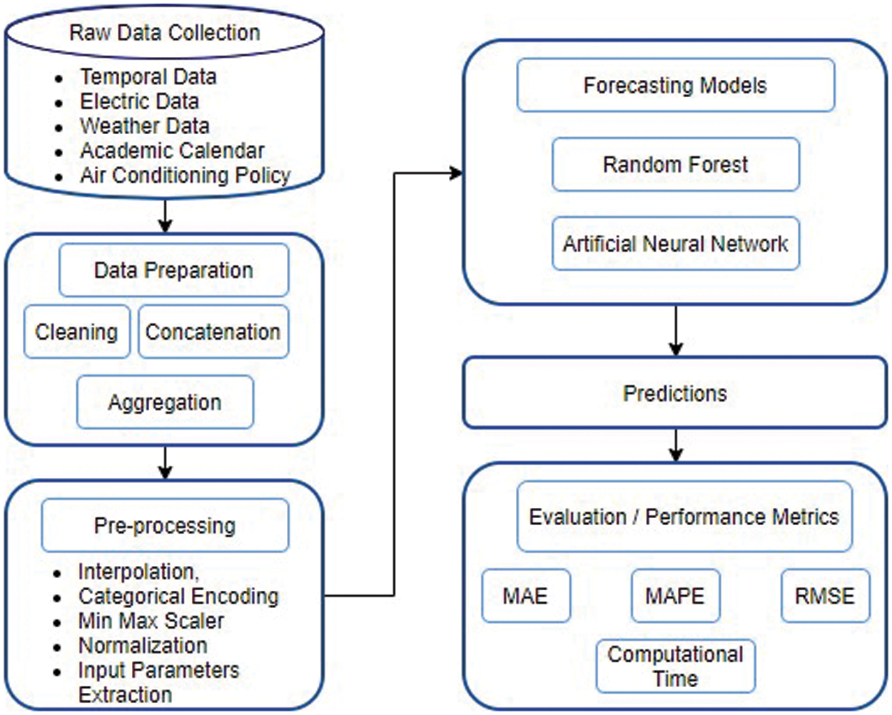
Figure 1: Proposed architecture for short-term energy forecasting
In the first step, raw electricity data is collected for every working day of the university at 20-s intervals. The collected raw data is aggregated to every minute, 15-min and 1-h granularity. The daily weather data is interpolated accordingly for each dataset. The categorical data is then encoded and added to the final data set. From the finalized dataset, features are extracted and the data is then normalized. Next, the preprocessed data is fed to the forecasting models (Random Forest Regressor and ANN) for training towards electricity load forecasting. The performances of these models are assessed based on various performance metrics such as MAPE, MAE, RMSE, as well as computational time. Each step is further elaborated as follows.
3.1 Raw Data Collection and Description
The electrical substation load which is under observation comprises of Services Department, National Incubation Center (NIC), Civil Engineering Department classes, office of Student Affairs, Directorate of Industrial Liaison (DIL), Student Cafeteria and Medical Department at NED University of Engineering and Technology. The area covered by Services Department, NIC, Civil Engineering Department, Office of Student Affairs, Directorate of Industrial Liaison, Student Cafeteria and Medical Department in terms of squared feet (sq. ft) is 3000, 18000, 12900, 2550, 2550, 5100, 4900 respectively as shown in Tab. 1 and marked its GIS location in Fig. 2. The total number of staff members in the services department is 35 with an average of 30 members present in the building every working day. In NIC, on an average daily basis, around 35 persons remain present in the building. In the Civil engineering department, there are 12 classrooms with 6 h of usage per day and accommodate approximately 45 students in a single slot. There are 14 labs with 4 h a day usage on average catering 35 students in an allotted time slot. The office of Student Affairs and DIL have 15 staff members each, with an average of 120 visitors daily.
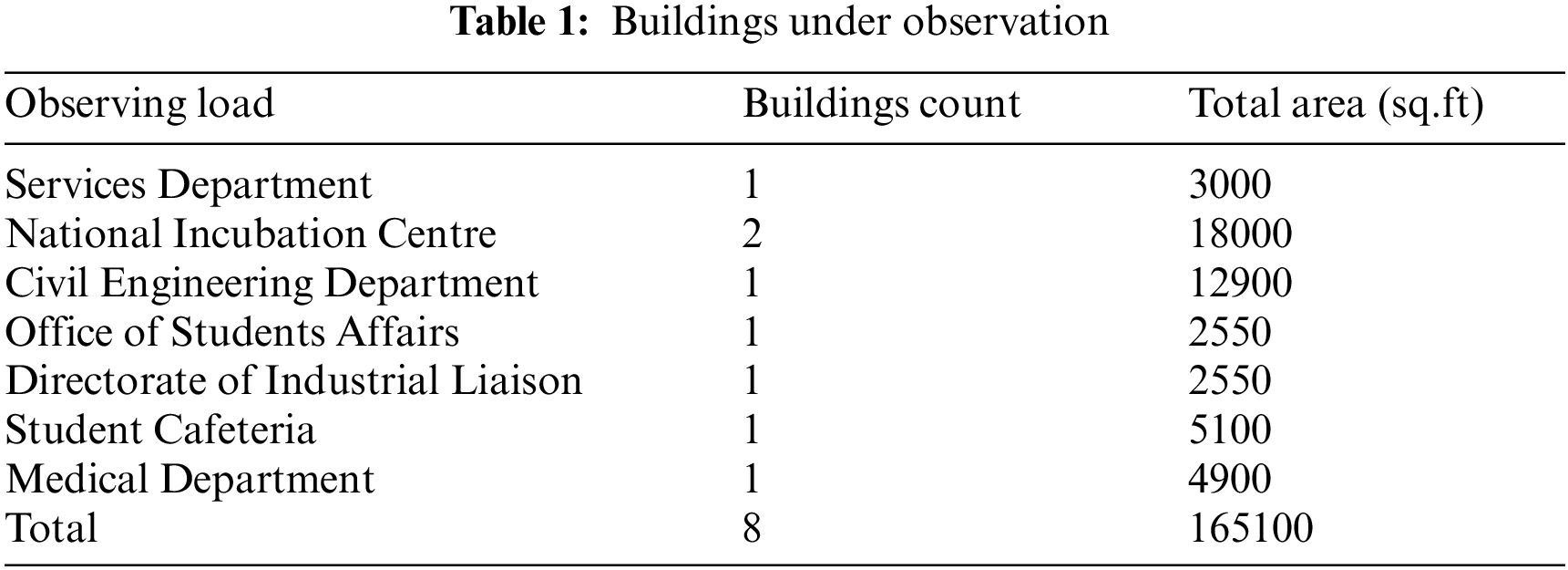
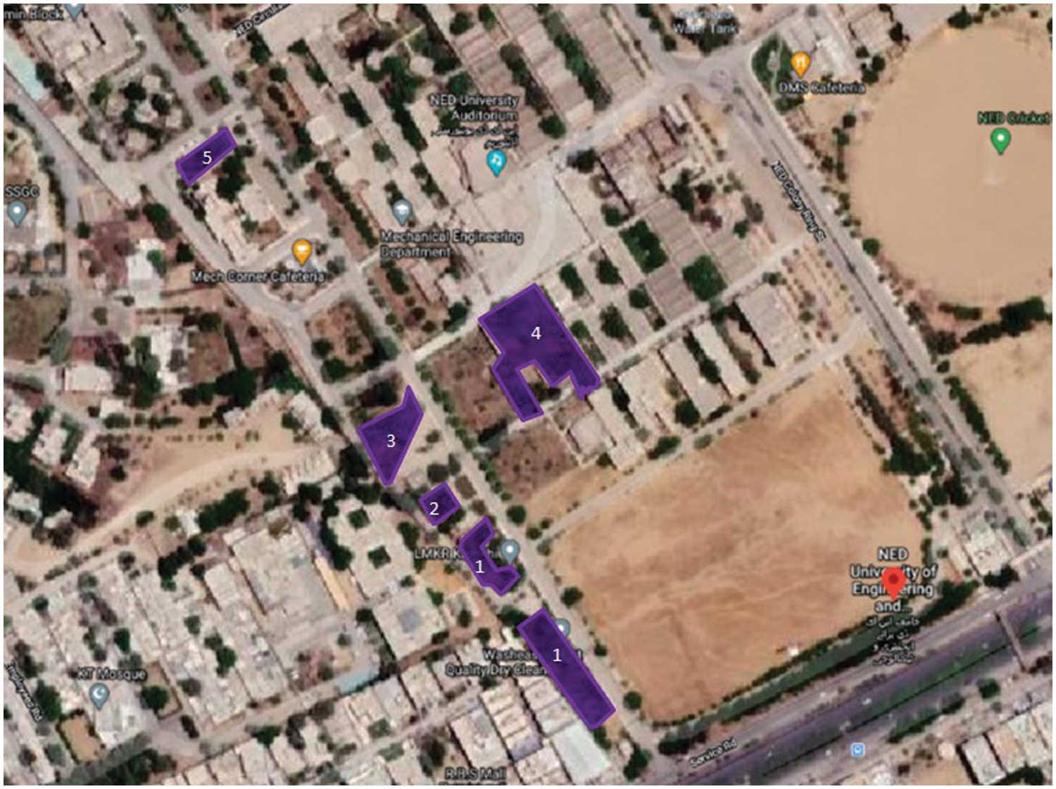
Figure 2: GIS location of buildings under observation; (1) National Incubation Centre (NIC), (2) Services department, (3) Office of student affairs, directorate of industrial liaison on 1st floor and student cafeteria on ground floor, (4) Civil engineering department, (5) Medical department
The Student Cafeteria has 10 employees with an average of 250 visitors. The number of staff members in the Medical Department is 8 with an approximately 60 visitors daily. These occupants influence the electricity consumption trend of selected buildings in a consistent manner. The raw data is collected based on parameters: temporal data, electricity data, weather data, university operations and AC policy. The temporal data consists of the month, day of the week, hour and minutes. Meteorologically, the weather transitioned from summers to winters to monsoon during the observed interval is also considered. In addition to power consumption, there is weather data for the same period as various seasonal changes affect electricity consumption [22,41]. Additionally, relevant data such as the academic calendar and air conditioning policy is also collected for the same period as depicted in Fig. 3.
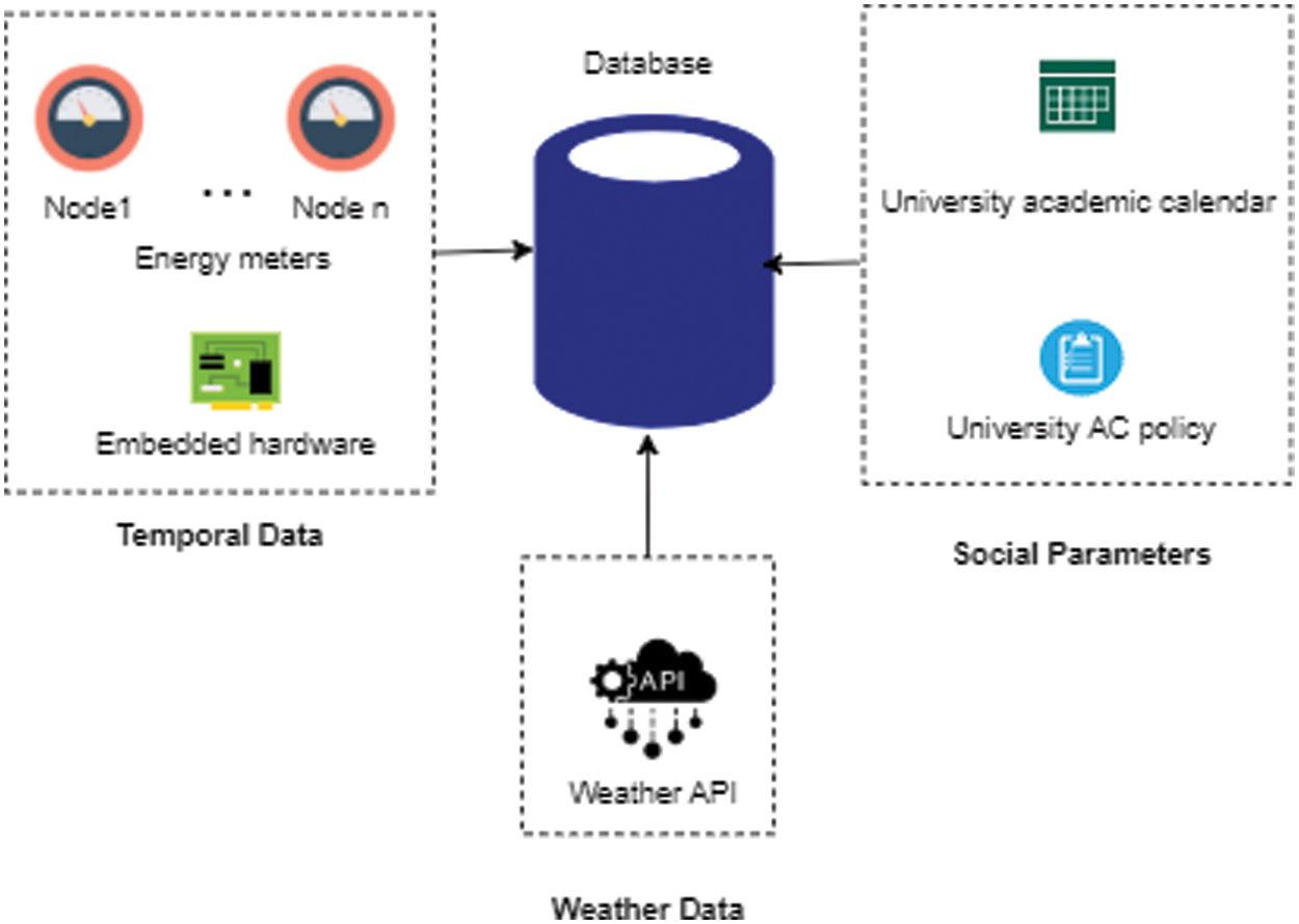
Figure 3: Data collection process
Real-time power consumption is monitored by the instrumentation center of the university through an indigenously built cloud-based real-time energy monitoring system. The hardware structure consists of three parts namely RS-485 module, main controller Arduino and ESP8266 Wi-Fi microchip. The RS-485 module is responsible for communicating with the energy analyzer. Energy analyzers are from different vendors like El-measure and Crompton. Once it gets all the 50 parameter values [42] from energy analyzer, the main controller fetches these values and sent it to the server using Wi-Fi communication module. The data is collected from Oct’2018 till Sept’2019 from 8:00 AM till 5:00 PM for each working day of the university.
3.2 Data Preparation & Preprocessing
Raw data represents power consumption of working days aggregated for minutely, 15-min and hourly granularities, during the full cycle (end of the fall semester, complete spring semester and beginning of the fall semester) where fall semester duration is from October till March and spring semester is from April till September. Occasionally, power consumption data may have interruptions due to different reasons, such as Wi-Fi connectivity issues or any electric instrument failure, etc. It results in outliers that need to be detected and calculated for accurate prediction. The daily weather data retrieved from an open-source weather API after a 3 h interval. It represents atmospheric temperature, humidity from the weather station deployed at the nearest location (Jinnah International Airport, Karachi). To cater to the absence of weather data, interpolation technique was deployed as mentioned in [24,42]. Generally, weather parameters are considered important when predicting short term load. The most widely used weather parameters are temperature and humidity. Correlation determination matrix is used to determine the dependence of parameters on one other. The matrix shown in Fig. 4 depicts the correlation between all possible pairs of our final dataset. The highest positive correlation of energy consumption is with temperature, followed by AC policy and humidity. The highest negative correlation of energy consumption is with the academic calendar, followed by the days of the week.
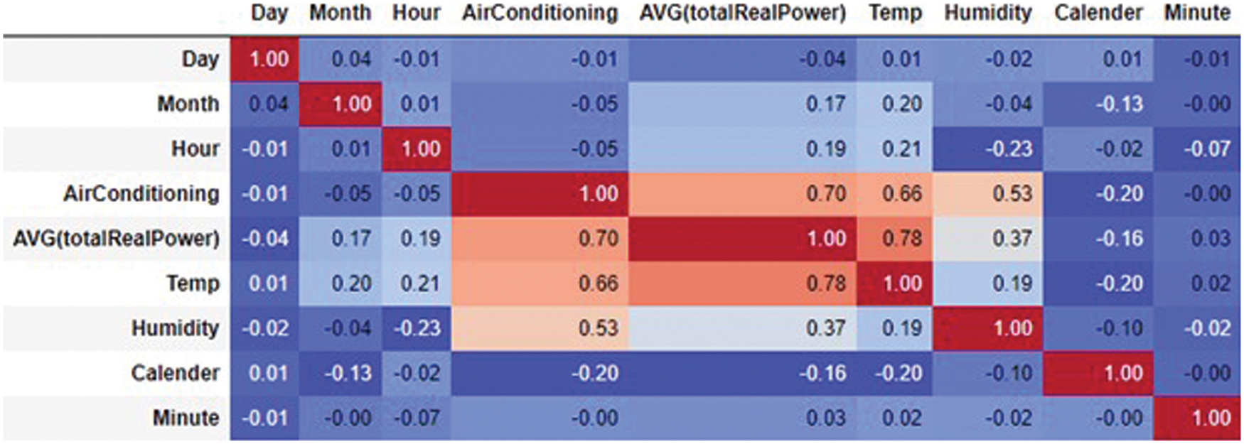
Figure 4: Correlation determination among the input parameters
Thus, according to our consumption dataset, the weather data is interpolated on minutes, 15-min and hourly granularities. Next, the dataset of consumption-related parameters and weather is concatenated and normalized using MinMaxScaler Algorithm. The MinMaxScaler algorithm scales each feature individually so that each feature comes within the range of the dataset. It normalizes the features individually so that each feature will have zero mean and unit standard deviation. Then, the categorical temporal data set is encoded using a one-hot encoder algorithm. One hot encoder is a characterization of categorical values into binary vectors. Finally, input parameters are extracted as follows. The time-series data of power consumption has the periodicity element. The temporal data set is broken down into months, days, hours and minutes for achieving the periodicity. If this periodicity is considered in the ML forecasting models, the predictions would be more accurate.
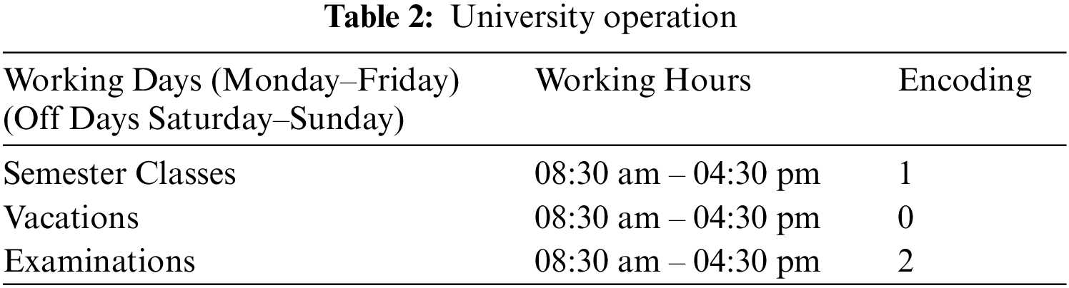
In most educational institutes, the classes and office activities are carried out fully in weekdays and partially (first half) in examination days. University is completely closed on the weekends along with exceptional holidays. This pattern is reflected in the ML model by encoding the data set with a range from 0 to 2, having 0 representing off-days, 1 for working days and 2 for examinations. Tab. 2 shows the sample of university operation details. Though, normally universities have clusters that contain administrative buildings for office work, classrooms for lectures and labs for practical, the working hours remain unchanged for the administration during vacations and examinations.
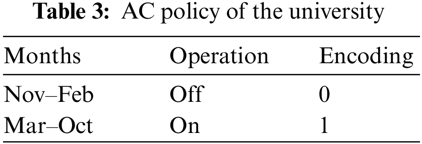
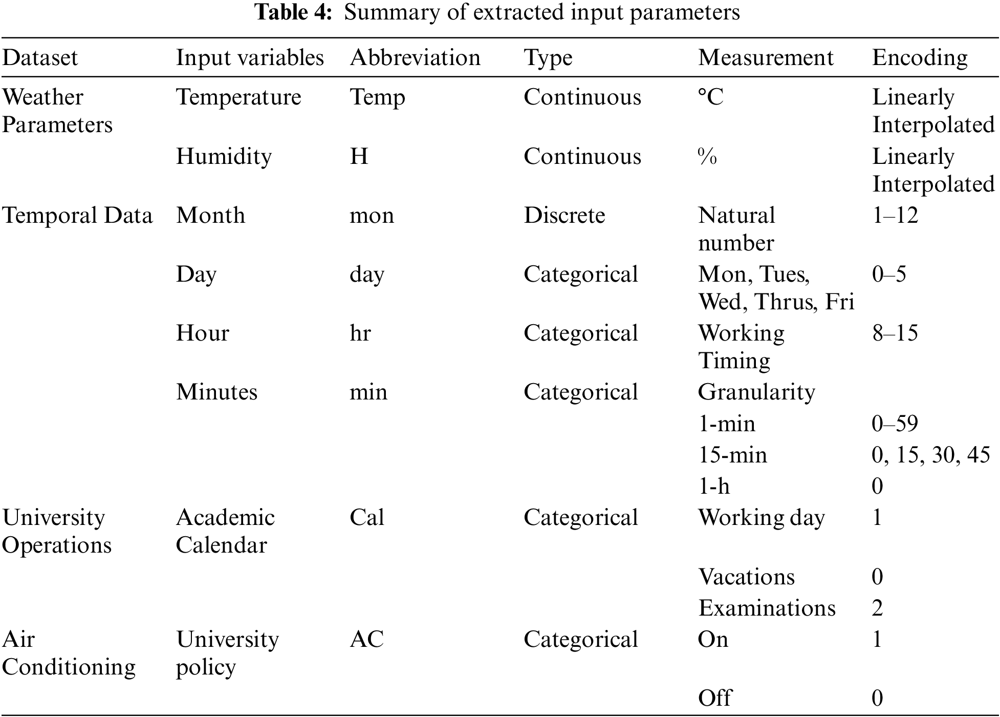
Tab. 3 shows the university AC policy details. To reflect this pattern on the ML model, the sequence is encoded into the data set with a range from 0 to 1 on an 8-dimensional features vector. Tab. 4 shows the full list of extracted features to be sent for training. The data set except for meteorological parameters are encoded using the one-hot encoder algorithm. The categorical variables are first mapped into integer values then each value is described as a binary vector with index 1 and rest of all as 0’s.
Development of the electricity load forecasting model is carried out by selecting two best-performing techniques, namely RF - a decision tree-based method and ANN - a neurons based method. For training, the dataset splits into training and validation datasets with a ratio of 70% to 30% respectively.
RF can be used as a classifier as well as a regressor and has the capability of running efficiently on a large amount of data for providing highly accurate results. As compared to other ML models, it requires lesser efforts for hyper-parameters tuning [16,33]. RF hyper parameters are its number of trees (n estimators), the maximum depth of the tree (max depth) and decision-related parameters such as a sample split and leaf node criteria. Number of features for the best split condition is set by using Eq. (1)
where, max_features is the number of features for the best split and n_features is the total number of features. When training RF, the optimal values for maximum depth and no. of the trees are found to be (max depth = 12, n estimators = 150) after a bunch of preliminary tests with different RF configurations. A subset of developed RF is shown in Fig. 5.
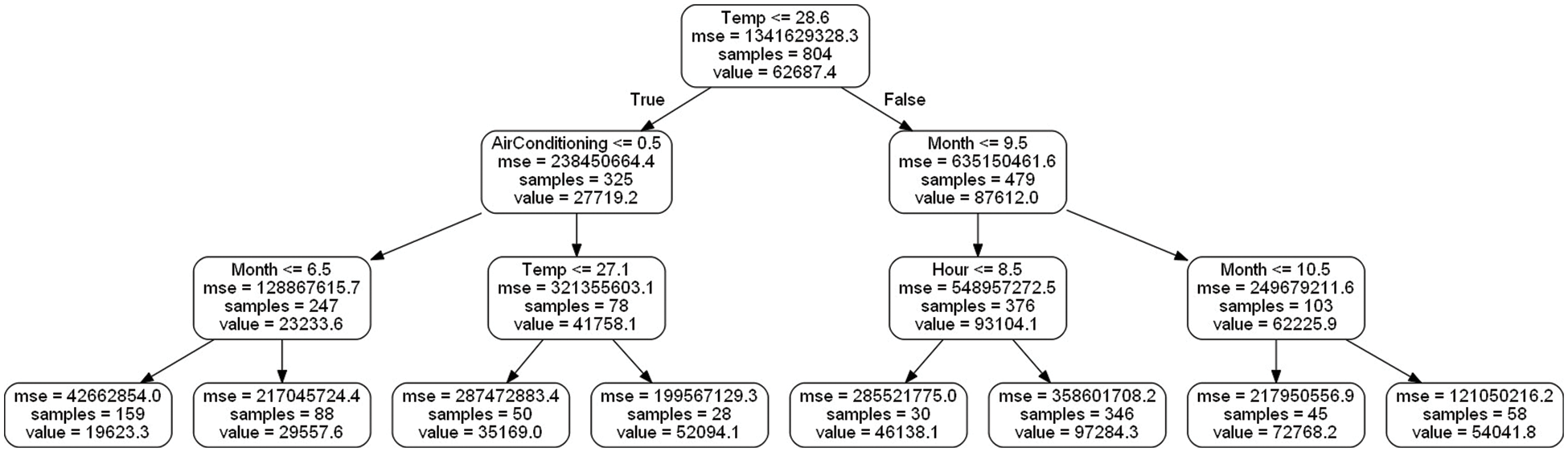
Figure 5: Architecture for a subset of proposed random forest
3.3.2 Artificial Neural Network
A typical neural network, also known as multi-layer perceptron (MLP), is a neuron based ML technique. It consists of a connected network of individual nodes known as perceptron, arranged in a series of layers [21,33]. ANN has three categorizations namely the input layer, hidden layer and output layer. The performance of any ANN depends upon the number of hidden layers, nodes in the layers and activation function. A neural network with more than two hidden layers, with a certain level of complexity to process sophisticated mathematical modelling of data, is defined as Deep Neural Network (DNN) [1,35]. This framework uses a 3 layered ANN as shown in Fig. 6.
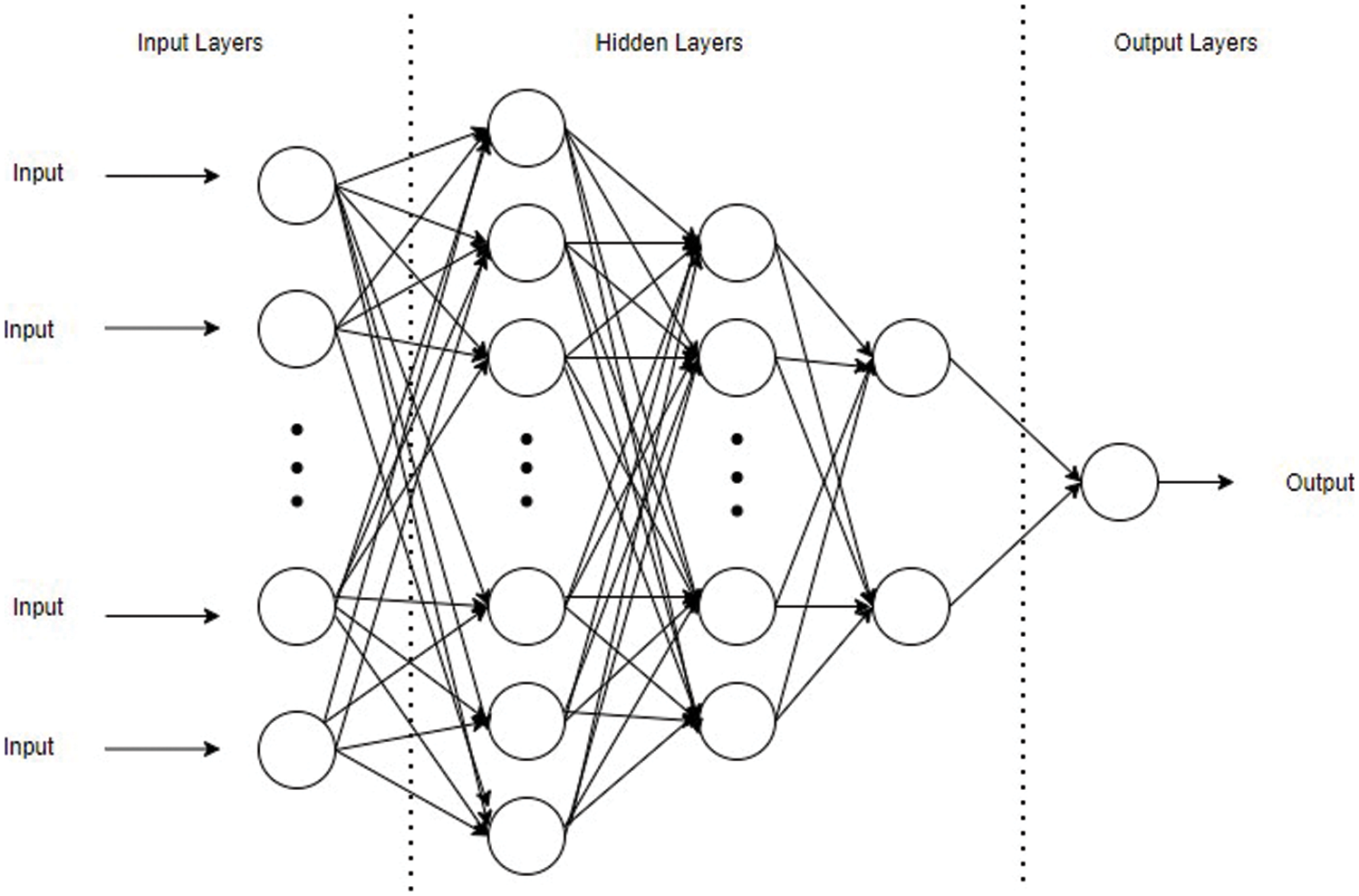
Figure 6: Architecture of proposed ANN
The three hidden layered ANN model having (128, 64, 32) neurons respectively is constructed. The ANN is trained using backpropagation with the rectified linear unit (ReLU) as the activation function for the hidden layers as defined in Eq. (2).
where, x is the input to the ReLU activation function f’(x).
3.4 Performance Evaluation Metrics
The performance of our proposed electricity load forecasting models is evaluated and compared with previously proposed approaches using Root Mean Square Error (RMSE), Mean Absolute Error (MAE), Mean Absolute Percentage Error (MAPE) and computational time. MAE calculates that how far predicted values are from observed values. It is calculated using Eq. (3).
where
MAPE is a measure of forecasting accuracy for fitted time series values. It is usually expressed in terms of percentage. It is calculated by using Eq. (5).
where
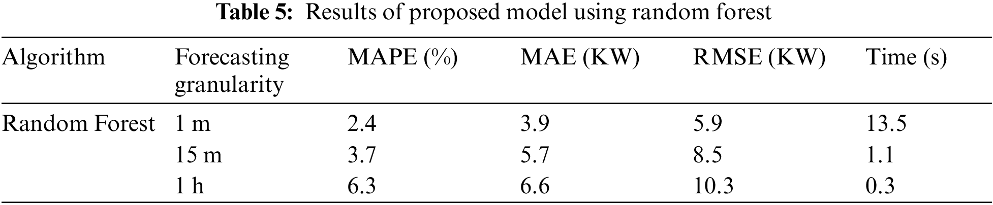
For the evaluation of our prediction models, several experiments were conducted on a one-year data collected for all working days of selected buildings of the university. The dataset is divided into a ratio of 70% to 30% for training and testing respectively and split randomly to break the sequential nature of the time-series dataset for accurate predictions. The values of performance metrics are calculated for each experiment to compare and select the optimal algorithm in terms of accuracy and computational time. During the training of ML algorithms, the model evaluation is categorized as under-fitting (large values of errors), over-fitting (i.e., learning of noise in the data) and good fit (i.e., the validation error is slightly higher than training error). The aim is to converge the model as a good fit. Thus, the prediction models require to be fine-tuned through experimentation. For RF, experiments were started by configuring a tree with max depth = 8 and n estimators = 50, both parameters were gradually increased for a good fit, max depth with a step of 2 and n estimators with a step of 50 until optimal results were found with (max depth = 12, n estimators = 150).
Tab. 5 shows the results of proposed model using optimal RF in terms of chosen performance metrics. The performance (i.e., sensitivity) of ANN depends upon different number of hidden layers. However, there is no general rule of thumb for deciding no. of layers or no. of neurons in the hidden layer. It may vary with the nature of the application, depending upon the amount of dataset, its quality and training parameters. The development of ANN model was started with two hidden layers having (64,32) neurons respectively, then gradually increased no. of layers and neurons to find the optimal value of hidden layers and neurons. The optimal composition for our dataset was found to be an ANN of 3 hidden layers with (128,64,32) neurons respectively built through 500 epochs.
Tab. 6 shows the performance metrics of optimal ANN on our dataset. Figs. 7 and 8 show the predicted results against the actual observed values while using the trained forecasting models.
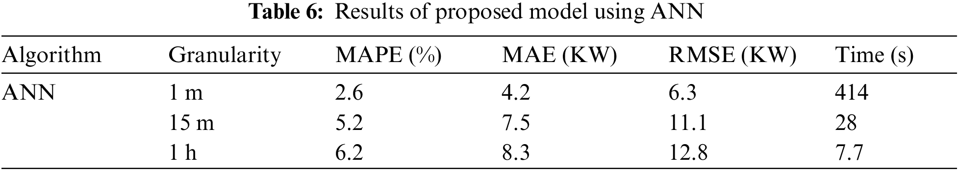
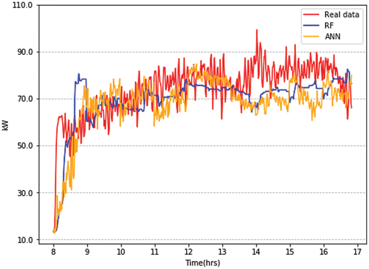
Figure 7: Electricity load prediction using proposed models for working day of the university when the air conditioning is allowed
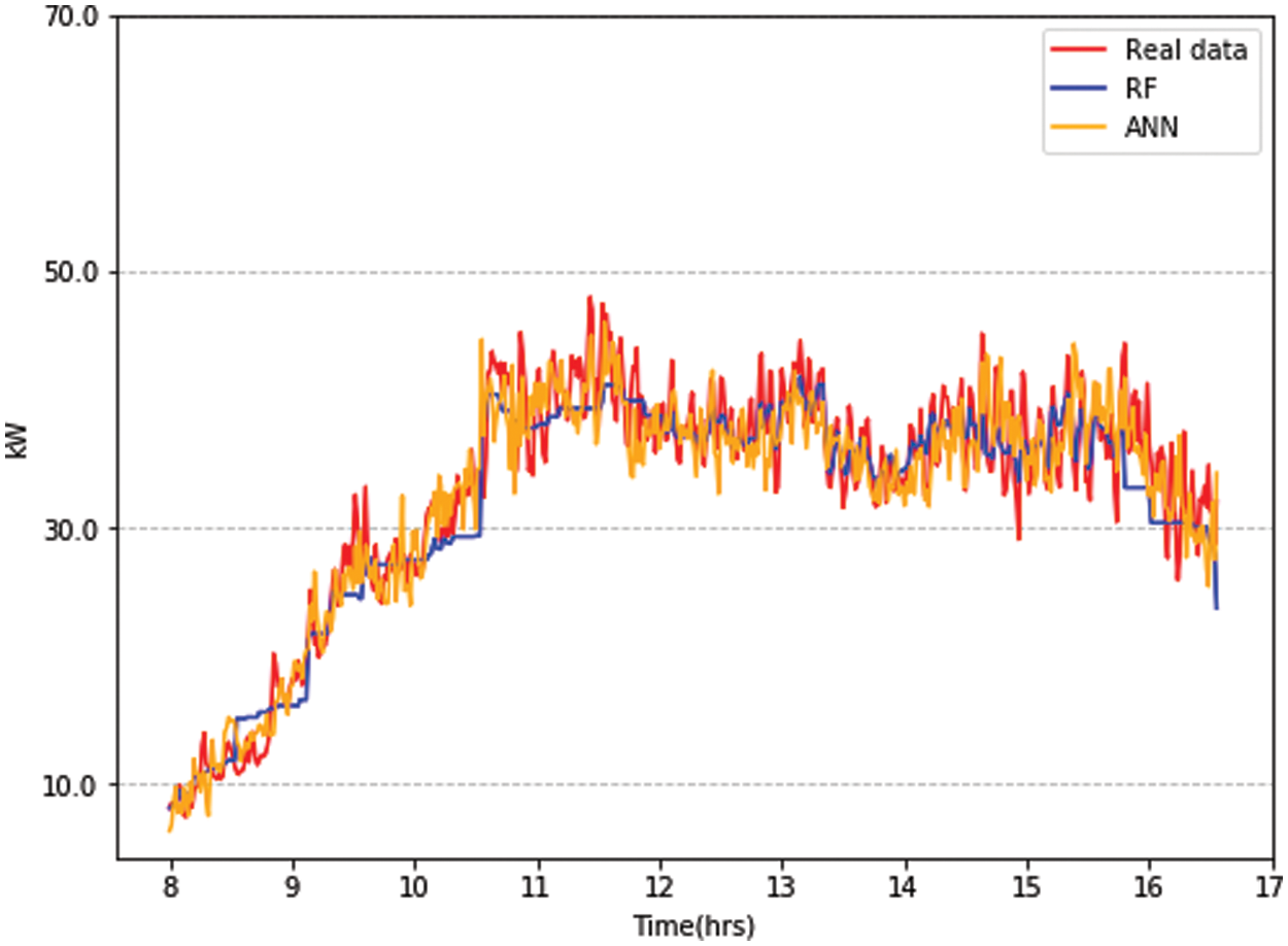
Figure 8: Electricity load prediction using proposed models for vacation day of the university’s students when the air conditioning is not allowed
Fig. 9 visualizes the results in terms of calculated performance metrics. It reveals that in terms of MAPE, RF performed better except for the 1-h dataset where ANN outperforms. In terms of MAE, both models are comparative while RSME shows that RF outperformed ANN. Concerning computational time RF is approximately 25 times faster than ANN in all three datasets granularities.
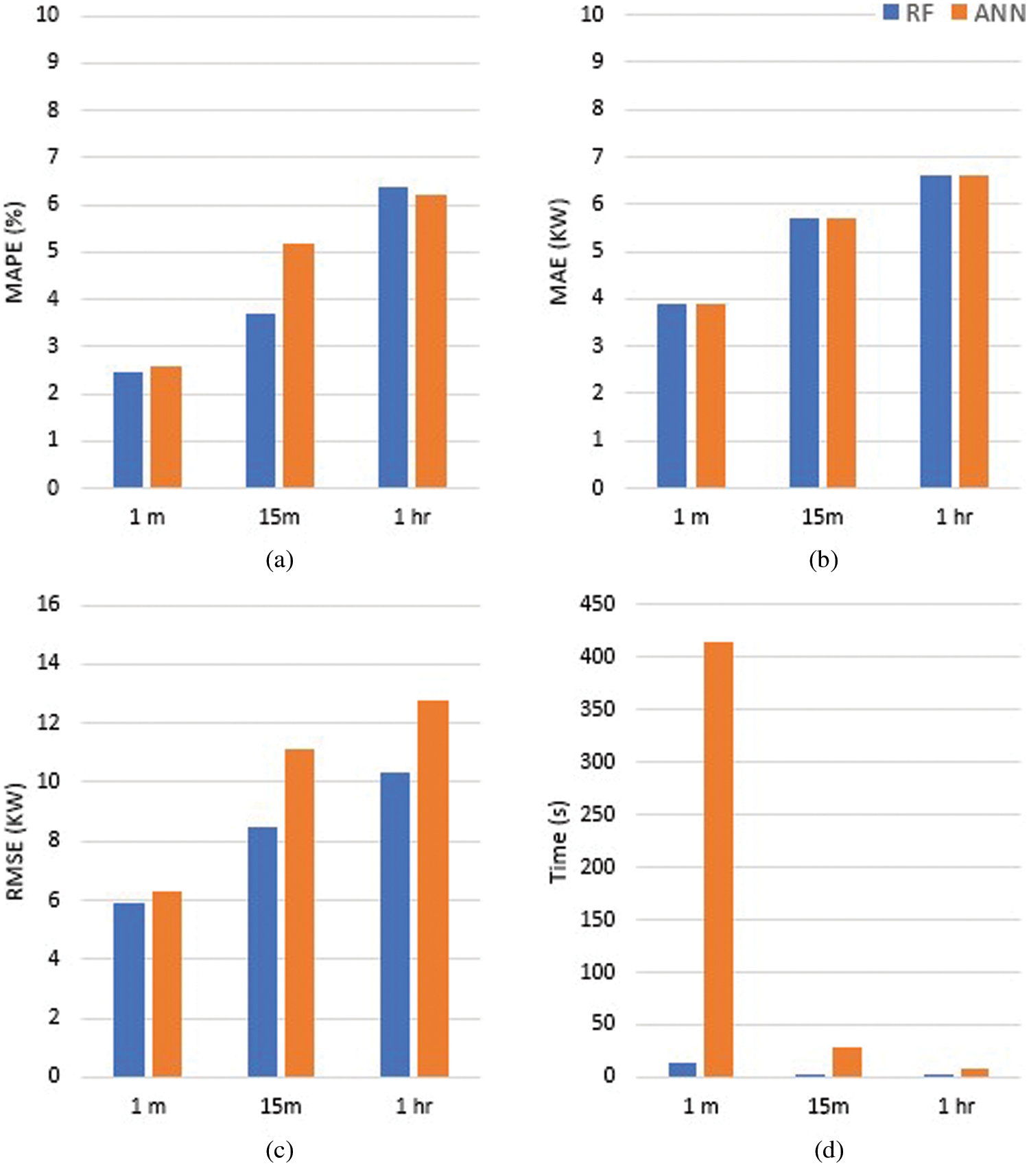
Figure 9: Results of RF and ANN in terms of performance metrics (a) MAPE, (b) MAE, (c) RMSE, (d) Time
Speed and accuracy often stand on opposite sides, there arises a need for obtaining an optimal trade-off between both. Thus, the proposed methodology investigates accurate yet time-efficient ML algorithms. For electricity load forecasting, computational time and accuracy are affected by the nature and quality of the dataset fed to it. The forecasting granularity, characteristics (linear or complex), behavior (sequential or chained) and type (categorical, discrete on continuous) of data, all contributes to the overall computational cost and accuracy of the ML algorithm. Since energy consumption is a real-time process the efficiency of the ML algorithm is important for live inference. That’s why well prepared and pre-processed datasets with reduced parameters were fed as input to the proposed algorithms for enhanced efficiency with reduced computational time. The performance of both proposed models was analyzed in terms of accuracy as well as computational time for 1-min, 15-min and 1-h forecasting granularity. The proposed models were trained and evaluated with full and reduced input parameters for each granularity. They were compared with each other as well as with other previously reported techniques in the open literature.
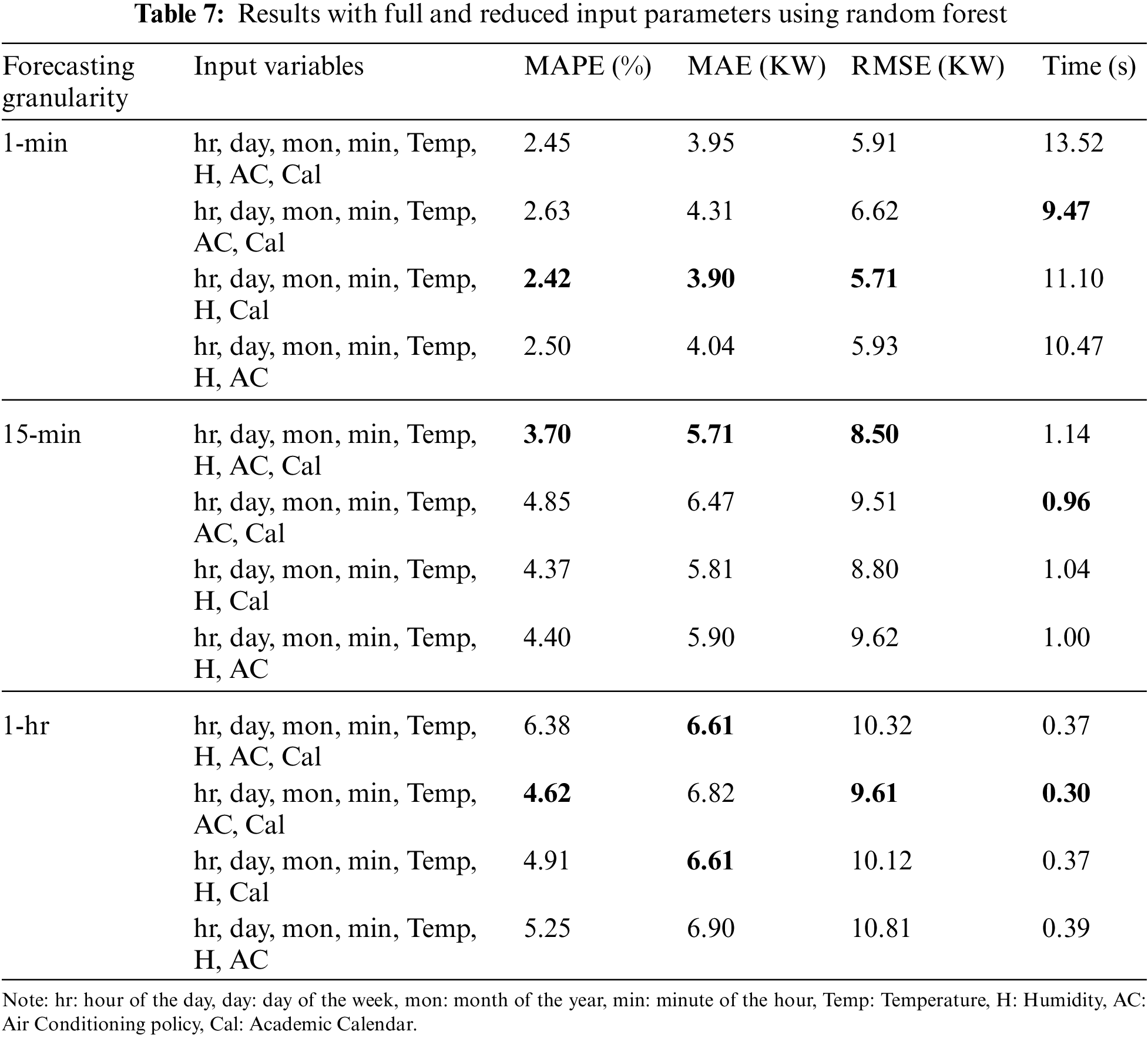
Tab. 7 shows the results with full and reduced input parameters using RF. The first row for 1-min, 15-min and 1-h granularity shows the performance of the model considering all input parameters. Then second, third and fourth rows are listed with reduced input parameters. All the metrics were calculated for all cases on the same dataset. It is clearly shown that, for the 1-min granularity dataset, input parameters without the AC policy better performs for all performance metrics. For the 15-min granularity, the model performs better when all input parameters are given. For the 1-h granularity dataset, the model without humidity as an input variable gave better results as compared to the model with all input variables.
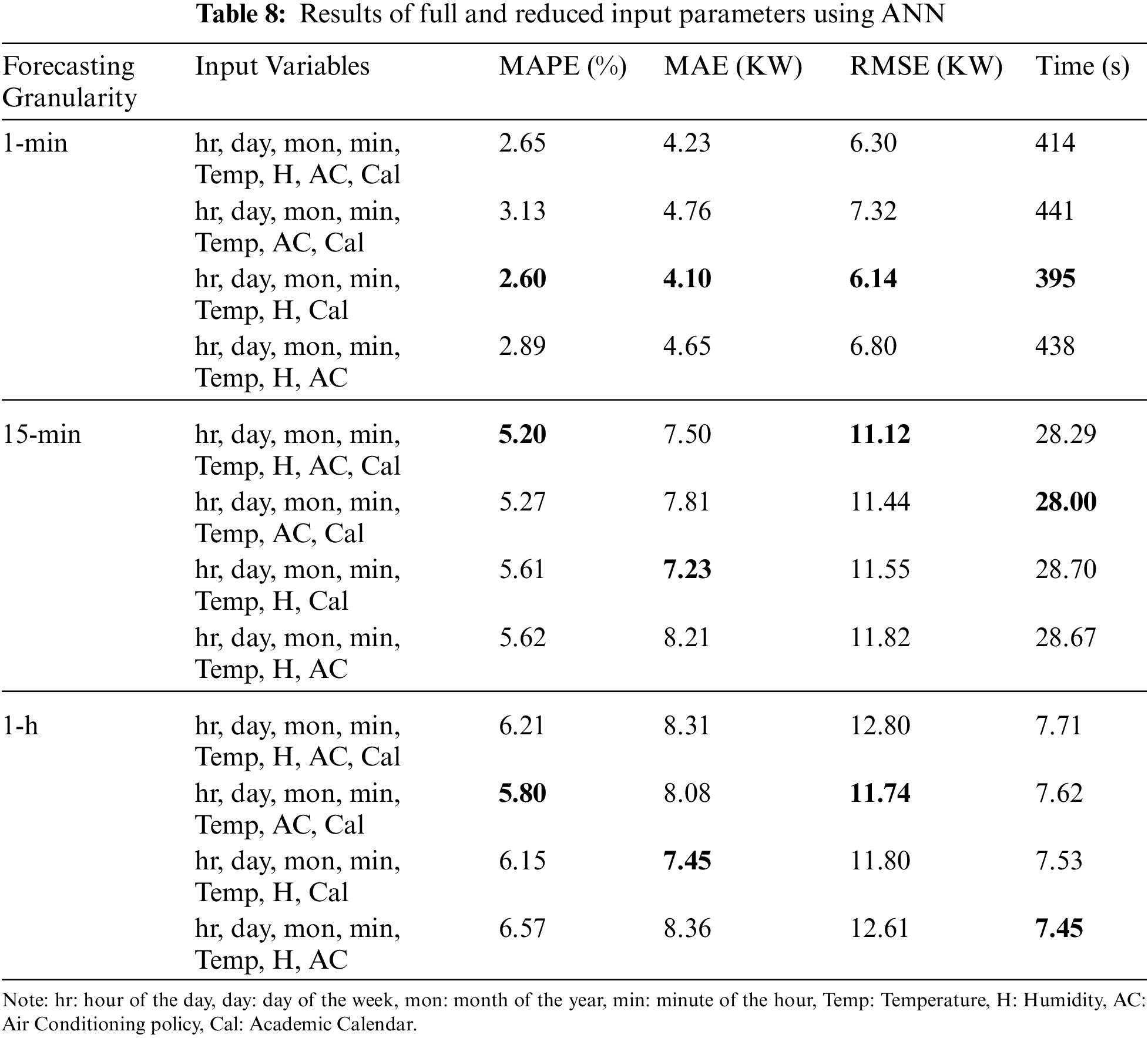
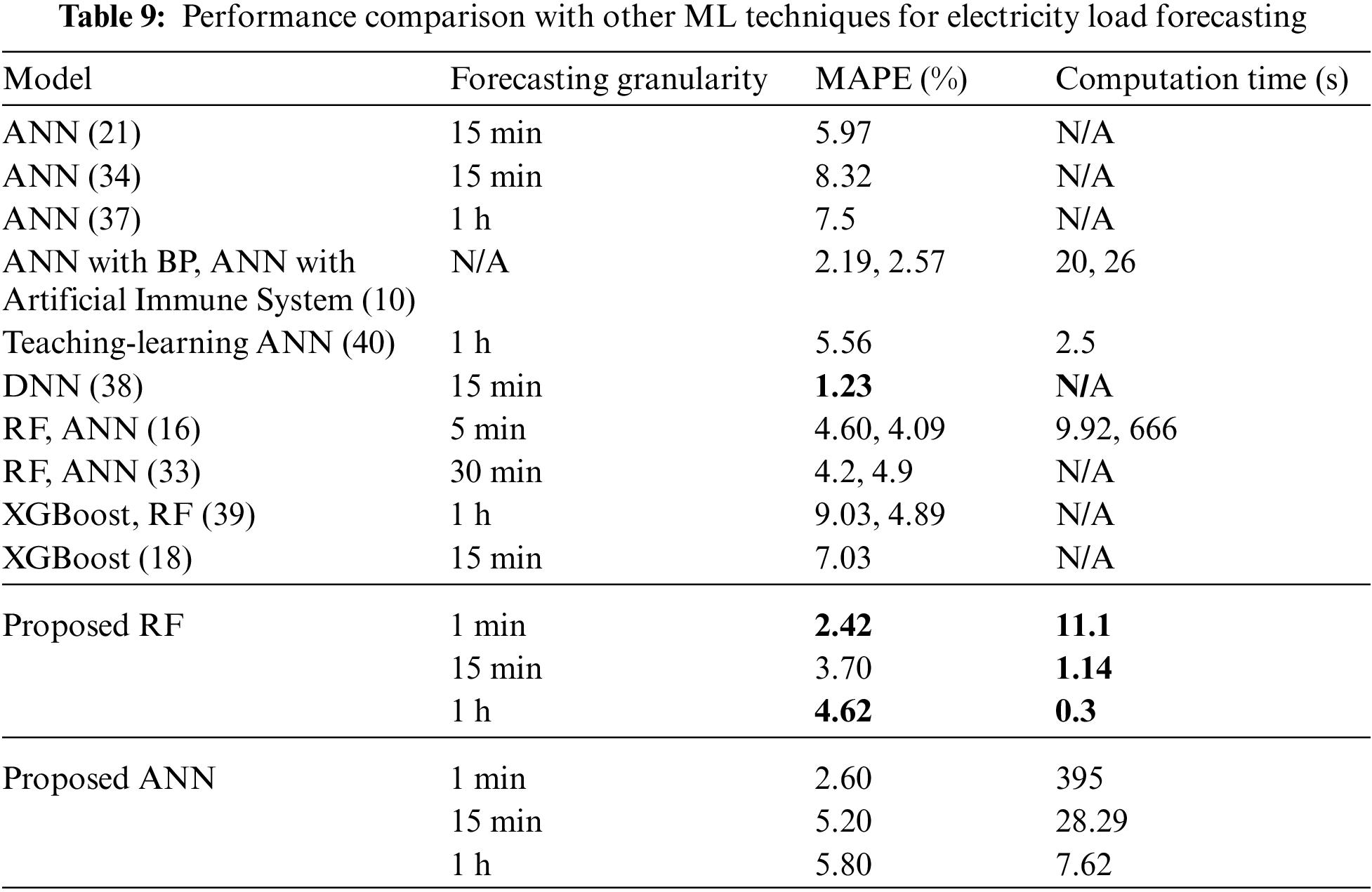
Tab. 8 shows the performance evaluation with full and reduced input parameters for ANN model. The same dataset was provided for all cases. All the datasets along with their evaluators show almost similar results as of the RF model. The comparison results show that for different forecasting granularity, the importance of input parameters slightly changes. It is found that temporal data is of higher importance followed by weather parameters and social variables. Tab. 9 compares the performance with other ML models reported in open literature for electricity load forecasting. It provide details of modelling time and error in terms of MAPE for their respective data granularities. In terms of accuracies of 1-min and 1-h granularity, proposed RF outperformed previously proposed models whereas in the 15-min granularity proposed RF is close to competing techniques but DNN [38] showed better results at an additional expense of computational time, thus not suitable for real-time usage. However, in terms of computational time, proposed RF model took less time as compared to previous models. Thus, if accuracy and computational time are simultaneously considered for real-time application, RF outperformed all other techniques.
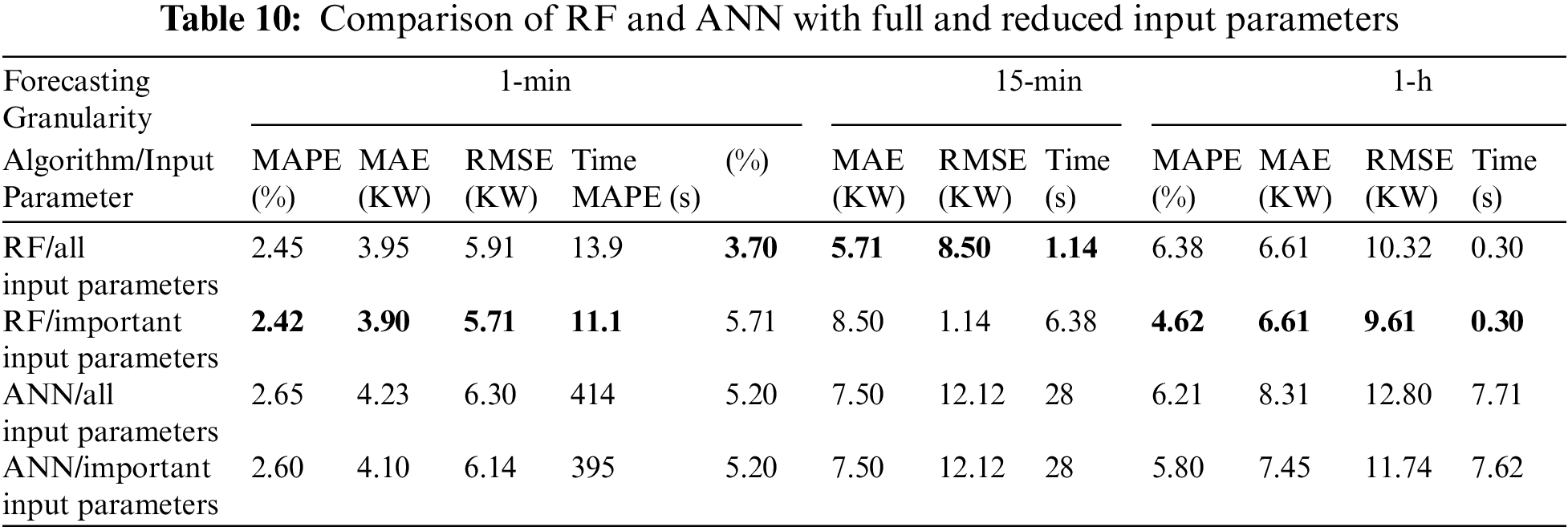
Tab. 10 compares the performance of proposed models with full and reduced input parameters respectively. It indicates that at all granularities, the RF model performs better in terms of accuracy as well as computation time. RF performs slightly better in terms of MAPE, MAE and RMSE and Time. Both models show their robustness in learning in terms of accuracy and it is concluded that both models can be used for effective prediction. However, RF proved to be faster than the ANN. The proposed optimal solution is well suited for integrating with a live energy monitoring system. It will help the building administration and energy managers in making real-time informed decisions, real-time pricing and successful integration of renewable energy resources to the existing system.
In future, the same model can be used for the short-term prediction of electricity consumption of residential or commercial areas. The proposed models can also be used for the predictions on any data set other than electricity consumption that is for transfer learning. With some changes in the proposed architecture of the ANN and RF model, as well as the availability of the dataset it may be extended for the long-term prediction of electricity consumption.
This study focused on data preprocessing with complete, partial and reduced extracted input parameters aiming to develop an optimal ML based short-term electricity consumption forecasting. Performances of ANN and RF techniques were evaluated in terms of the widely used performance metrics. Based on MAPE, MAE, RMSE, the study found that for the 1-min and 15-min and 1-h forecasting granularity windows, RF model with different sets of reduced and full input parameters performed better as compared to ANN. The results are indicative that the forecasting granularity and input parameters of data available impact performance accuracies differently for ANN and RF models. In terms of computational time towards algorithms convergence, RF model was observed to be faster for all datasets. Both models are competitive with each other and are applicable in the domain of real-time energy consumption forecasting of buildings. In the next steps, the proposed optimal solution is planned for integration with live energy monitoring system. Such a system will help the energy managers in taking real-time informed decisions, real-time projected costs, and successful integration of renewable energy resources to the existing system. The system will also help HEI administration for developing institutional policies for minimizing electricity cost.
Funding Statement: This research is funded by Neurocomputation Lab, National Center of Artificial Intelligence, NED University of Engineering and Technology, Karachi, 75270, Pakistan (PSDP.263/2017-18).
Conflicts of Interest: The authors declare that they have no known competing financial interests or personal relationships that could have appeared to influence the work reported in this paper.
1. K. Amarasinghe, D. Marino and M. Manic, “Deep neural networks for energy load forecasting,” in 2017 IEEE 26th Int. Sym. on Industrial Electronics (ISIE), Edinburgh, UK, 2017. [Google Scholar]
2. S. Ryu, J. Noh and H. Kim, “Deep neural network based demand side short term load forecasting,” Energies, vol. 10, no. 1, p. 3, 2016. [Google Scholar]
3. E. González-Romera, M. Jaramillo-Morán and D. Carmona-Fernández, “Monthly electric energy demand forecasting with neural networks and Fourier series,” Energy Conversion and Management, vol. 49, no. 11, pp. 3135–3142, 2008. [Google Scholar]
4. A. Motamedi, H. Zareipour and W. Rosehart, “Electricity price and demand forecasting in smart grids,” IEEE Transactions on Smart Grid, vol. 3, no. 2, pp. 664–674, 2012. [Google Scholar]
5. S. Yao, Y. Song, L. Zhang and X. Cheng, “Wavelet transform and neural networks for short-term electrical load forecasting,” Energy Conversion and Management, vol. 41, no. 18, pp. 1975–1988, 2000. [Google Scholar]
6. G. Oğcu, O. Demirel and S. Zaim, “Forecasting electricity consumption with neural networks and support vector regression,” Procedia Social and Behavioral Sciences, vol. 58, pp. 1576–1585, 2012. [Google Scholar]
7. U. Basaran and M. Kurban, “A new approach for the short-term load forecasting with autoregressive and artificial neural network models,” International Journal of Computational Intelligence Research, vol. 3, no. 1, pp. 66–71, 2007. [Google Scholar]
8. J. Kumaran and G. Ravi, “Long-term sector-wise electrical energy forecasting using artificial neural network and biogeography-based optimization,” Electric Power Components and Systems, vol. 43, no. 11, pp. 1225–1235, 2015. [Google Scholar]
9. G. Tso and K. Yau, “Predicting electricity energy consumption: A comparison of regression analysis, decision tree and neural networks,” Energy, vol. 32, no. 9, pp. 1761–1768, 2007. [Google Scholar]
10. M. Hamid and T. Rahman, “Short term load forecasting using an artificial neural network trained by artificial immune system learning algorithm,” in 2010 12th Int. Conf. on Computer Modelling and Simulation, Cambridge, UK, 2010. [Google Scholar]
11. M. Mat Daut, M. Hassan, H. Abdullah, H. Rahman, M. Abdullah et al., “Building electrical energy consumption forecasting analysis using conventional and artificial intelligence methods: A review,” Renewable and Sustainable Energy Reviews, vol. 70, no. 8, pp. 1108–1118, 2017. [Google Scholar]
12. F. Kaytez, M. Taplamacioglu, E. Cam and F. Hardalac, “Forecasting electricity consumption: A comparison of regression analysis, neural networks and least squares support vector machines,” International Journal of Electrical Power & Energy Systems, vol. 67, no. 1, pp. 431–438, 2015. [Google Scholar]
13. M. Mohandes, “Support vector machines for short-term electrical load forecasting,” International Journal of Energy Research, vol. 26, no. 4, pp. 335–345, 2002. [Google Scholar]
14. V. Bianco, O. Manca and S. Nardini, “Electricity consumption forecasting in Italy using linear regression models,” Energy, vol. 34, no. 9, pp. 1413–1421, 2009. [Google Scholar]
15. G. Tso and K. Yau, “Predicting electricity energy consumption: A comparison of regression analysis, decision tree and neural networks,” Energy, vol. 32, no. 9, pp. 1761–1768, 2007. [Google Scholar]
16. M. Ahmad, M. Mourshed and Y. Rezgui, “Trees vs Neurons: Comparison between random forest and ANN for high-resolution prediction of building energy consumption,” Energy and Buildings, vol. 147, no. 1, pp. 77–89, 2017. [Google Scholar]
17. S. Walker, W. Khan, K. Katic, W. Maassen and W. Zeiler, “Accuracy of different machine learning algorithms and added-value of predicting aggregated-level energy performance of commercial buildings,” Energy and Buildings, vol. 209, p. 109705, 2020. [Google Scholar]
18. A. Kharal, A. Mahmood and K. Ullah, “Load forecasting of an educational institution using machine learning: the case of Nust, Islamabad,” Pakistan Journal of Science, vol. 71, no. 4, pp. 252–257, 2020. [Google Scholar]
19. Z. Yu, F. Haghighat, B. Fung and H. Yoshino, “A decision tree method for building energy demand modeling,” Energy and Buildings, vol. 42, no. 10, pp. 1637–1646, 2010. [Google Scholar]
20. T. Hong, C. Koo and K. Jeong, “A decision support model for reducing electric energy consumption in elementary school facilities,” Applied Energy, vol. 95, no. 3, pp. 253–266, 2012. [Google Scholar]
21. J. Moon, J. Park, E. Hwang and S. Jun, “Forecasting power consumption for higher educational institutions based on machine learning,” The Journal of Supercomputing, vol. 74, no. 8, pp. 3778–3800, 2017. [Google Scholar]
22. A. Azadeh, S. Ghaderi and S. Sohrabkhani, “Forecasting electrical consumption by integration of Neural Network, time series and ANOVA,” Applied Mathematics and Computation, vol. 186, no. 2, pp. 1753–1761, 2007. [Google Scholar]
23. K. Kandananond, “Forecasting electricity demand in Thailand with an artificial neural network approach,” Energies, vol. 4, no. 8, pp. 1246–1257, 2011. [Google Scholar]
24. A. Azadeh, S. Ghaderi and S. Sohrabkhani, “A simulated-based neural network algorithm for forecasting electrical energy consumption in Iran,” Energy Policy, vol. 36, no. 7, pp. 2637–2644, 2008. [Google Scholar]
25. A. Neto and F. Fiorelli, “Comparison between detailed model simulation and artificial neural network for forecasting building energy consumption,” Energy and Buildings, vol. 40, no. 12, pp. 2169–2176, 2008. [Google Scholar]
26. H. Daneshi, M. Shahidehpour and A. Choobbari, “Long-term load forecasting in electricity market,” in IEEE Int. Conf. on Electro/Information Technology, IEEE, Ames, IA, USA, 2008. [Google Scholar]
27. G. Escrivá-Escrivá, C. Álvarez-Bel, C. Roldán-Blay and M. Alcázar-Ortega, “New artificial neural network prediction method for electrical consumption forecasting based on building end-uses,” Energy and Buildings, vol. 43, no. 11, pp. 3112–3119, 2011. [Google Scholar]
28. Y. Chae, R. Horesh, Y. Hwang and Y. Lee, “Artificial neural network model for forecasting sub-hourly electricity usage in commercial buildings,” Energy and Buildings, vol. 111, no. 1, pp. 184–194, 2016. [Google Scholar]
29. F. Ardakani and M. Ardehali, “Long-term electrical energy consumption forecasting for developing and developed economies based on different optimized models and historical data types,” Energy, vol. 65, no. 1, pp. 452–461, 2014. [Google Scholar]
30. L. Ekonomou, “Greek long-term energy consumption prediction using artificial neural networks,” Energy, vol. 35, no. 2, pp. 512–517, 2010. [Google Scholar]
31. C. Deb, L. Eang, J. Yang and M. Santamouris, “Forecasting diurnal cooling energy load for institutional buildings using Artificial Neural Networks,” Energy and Buildings, vol. 121, pp. 284–297, 2016. [Google Scholar]
32. A. Ahmad, M. Hassan, M. Abdullah, H. Rahman, F. Hussin et al., “A review on applications of ANN and SVM for building electrical energy consumption forecasting,” Renewable and Sustainable Energy Reviews, vol. 33, no. 10, pp. 102–109, 2014. [Google Scholar]
33. J. Moon, Y. Kim, M. Son and E. Hwang, “Hybrid short-term load forecasting scheme using random forest and multilayer perceptron,” Energies, vol. 11, no. 12, pp. 3283, 2018. [Google Scholar]
34. J. Moon, S. Park, S. Rho and E. Hwang, “A comparative analysis of artificial neural network architectures for building energy consumption forecasting,” International Journal of Distributed Sensor Networks, vol. 15, no. 9, p. 155014771987761, 2019. [Google Scholar]
35. C. Huang and P. Kuo, “A deep CNN-LSTM model for particulate matter (PM2.5) forecasting in smart cities,” Sensors, vol. 18, no. 7, p. 2220, 2018. [Google Scholar]
36. D. Marino, K. Amarasinghe and M. Manic, “Building energy load forecasting using Deep Neural Networks,” in IECON, 2016 - 42nd Ann. Conf. of the IEEE Industrial Electronics Society, Florence, Italy, 2016. [Google Scholar]
37. Y. Kim, H. Son and S. Kim, “Short term electricity load forecasting for institutional buildings,” Energy Reports, vol. 5, no. 3, pp. 1270–1280, 2019. [Google Scholar]
38. N. Bendaoud and N. Farah, “Using deep learning for short-term load forecasting,” Neural Computing and Applications, vol. 32, no. 18, pp. 15029–15041, 2020. [Google Scholar]
39. L. Cao, Y. Li, J. Zhang, Y. Jiang, Y. Han et al., “Electrical load prediction of healthcare buildings through single and ensemble learning,” Energy Reports, vol. 6, no. 19, pp. 2751–2767, 2020. [Google Scholar]
40. K. Li, X. Xie, W. Xue, X. Dai, X. Chen et al., “A hybrid teaching-learning artificial neural network for building electrical energy consumption prediction,” Energy and Buildings, vol. 174, no. 6, pp. 323–334, 2018. [Google Scholar]
41. P. Mandal, T. Senjyu, N. Urasaki and T. Funabashi, “A neural network based several-hour-ahead electric load forecasting using similar days approach,” International Journal of Electrical Power & Energy Systems, vol. 28, no. 6, pp. 367–373, 2006. [Google Scholar]
42. Elmeasure, “Programming Guide V3,” 2017. [Online]. Available: https://www.elmeasure.com/storage/app/media/resources/documents/elmeasure-multifunction-meter-multifunction2r-programming-guide.pdf. [Google Scholar]
 | This work is licensed under a Creative Commons Attribution 4.0 International License, which permits unrestricted use, distribution, and reproduction in any medium, provided the original work is properly cited. |