DOI:10.32604/cmc.2022.027847
| Computers, Materials & Continua DOI:10.32604/cmc.2022.027847 | |
| Article |
An Optimal Method for High-Resolution Population Geo-Spatial Data
Department of Disaster Management, Al-Balqa Applied University, Prince Al-Hussien Bin Abdullah II Academy for Civil Protection, Jordan
*Corresponding Author: Rami Sameer Ahmad Al Kloub. Email: rami.kloub@bau.edu.jo
Received: 27 January 2022; Accepted: 31 March 2022
Abstract: Mainland China has a poor distribution of meteorological stations. Existing models’ estimation accuracy for creating high-resolution surfaces of meteorological data is restricted for air temperature, and low for relative humidity and wind speed (few studies reported). This study compared the typical generalized additive model (GAM) and autoencoder-based residual neural network (hereafter, residual network for short) in terms of predicting three meteorological parameters, namely air temperature, relative humidity, and wind speed, using data from 824 monitoring stations across China’s mainland in 2015. The performance of the two models was assessed using a 10-fold cross-validation procedure. The air temperature models employ basic variables such as latitude, longitude, elevation, and the day of the year. The relative humidity models employ air temperature and ozone concentration as covariates, while the wind speed models use wind speed coarse-resolution reanalysis data as covariates, in addition to the fundamental variables. Spatial coordinates represent spatial variation, while the time index of the day captures time variation in our spatiotemporal models. In comparison to GAM, the residual network considerably improved prediction accuracy: on average, the coefficient of variation (CV) R2 of the three meteorological parameters rose by 0.21, CV root-mean square (RMSE) fell by 37%, and the relative humidity model improved the most. The accuracy of relative humidity models was considerably improved once the monthly index was included, demonstrating that varied amounts of temporal variables are crucial for relative humidity models. We also spoke about the benefits and drawbacks of using coarse resolution reanalysis data and closest neighbor values as variables. In comparison to classic GAMs, this study indicates that the residual network model may considerably increase the accuracy of national high spatial (1 km) and temporal (daily) resolution meteorological data. Our findings have implications for high-resolution and high-accuracy meteorological parameter mapping in China.
Keywords: Machine learning; remote sensing; geography; disaster management; geo-spatial analysis
Meteorology is a basic variable that affects people’s production and life. In the field of ambient air pollution, meteorological factors such as temperature, relative humidity and wind speed, which affect the temporal and spatial distribution of pollutant concentrations such as ozone, PM2.5 and nitrogen oxides, are one of the important predictors [1–3]. In the agricultural field, the yield of crops, the development and reproduction of biological species, and agricultural disasters are inseparable from the meteorological environment [4]. One of the pests of apple grows and develops and improves its fecundity [5], and the increase in temperature aggravates the inhibitory effect of drought stress on the photosynthesis of Lycium barbarum in [6]. In terms of environmental health, meteorology is closely related to certain diseases. Reference [7] found that the distribution of hand, foot and mouth disease (HFMD) in mainland China has spatial heterogeneity, which is related to climate and socioeconomic variables. In the field of new energy, different terms of temperature and relative humidity, wind speed is also an important energy source that can provide electricity, and the distribution of wind energy resources can be explored through the study of wind speed [8,9]. In practical applications, the prediction of meteorological elements with high precision and high resolution is an important auxiliary decision-making information.
The ground meteorological monitoring sites in China are sparse and unevenly distributed. In 2015, there were only 824 monitoring sites in the country, and the number of sites in the eastern coastal and central regions was far more than that in the northwestern region. How to reliably estimate meteorological values at unmonitored sites from meteorological data at limited monitoring sites is extremely important for many applications. Among the three meteorological variables involved in this study, the research on rasterization of air temperature is the most. Direct interpolation methods are simple and common, such as Inverse Distance Weighting (IDW) [10,11], Origin Kriging (OK) [12,13], Co-Kriging (CK) [14,15], Spline-spline interpolation method [16,17], etc. The interpolation results have limited detail information when reflecting the small-scale climate change law [18]. In order to compensate for the station bias caused by sparse coverage, literature [19–21] used the point interpolation method based on BSHADE (Biased Sentinel Hospitals Areal Disease Estimation) to obtain an unbiased estimate with the smallest error variance. In addition to direct interpolation, there are also trend surface methods [22], multiple regression [23,24], etc., which incorporate macro-geographical factors as parameters into the construction of temperature models, which can effectively improve the simulation accuracy in a large-scale range [24]. It is a future development trend to consider factors related to temperature to improve the simulation accuracy of microscopic details of temperature distribution [25], such as adding elevation and NDVI information into the model [26,27]. In addition, rasterization of air temperature data using patterns is also under study [28]. There are also a few studies using artificial neural network [29], geographic weight regression [30], generalized linear regression [31], Bayesian maximum entropy model [32] to estimate air temperature. Although there is no lack of research on temperature rasterization, and some scholars are concerned about the change of wind speed in a long time series [33], the research on rasterization of relative humidity and wind speed is still very rare so far. In view of the sparseness of existing meteorological monitoring sites, the limitation of estimation methods in terms of accuracy, the lack of research on wind speed and relative humidity and the importance of their applications, this paper firstly analyzes the three meteorological elements of temperature, relative humidity and wind speed and their explanatory variables. Then, perform statistical analysis, and calculate the Pearson correlation coefficient for exploratory analysis, and combine different explanatory variable combinations to score the three meteorological factors. Furthermore, we build GAM and residual network models separately, determine the covariates of each meteorological model according to the results of the models, compare the differences between the meteorological distribution maps generated by the two models, and compare the results of the residual network model with ordinary Kriging interpolation. The results were compared with reanalysis data to verify their reliability.
2 Overview of the Study Area, Data Sources and Preprocessing
2.1 Overview of the Study Area
The study area is the mainland of China, excluding Taiwan province and the land in the Chinese seas. 9457700 km2. There are various types of climate in China. The eastern half has a large-scale monsoon climate, and the continental monsoon prevails in winter, which is cold and dry. The marine monsoon prevails in summer, which is hot and humid and rainy. The Qinghai-Tibet Plateau has a high altitude and a large area, forming a unique alpine climate. The northwest region is out of the reach of the marine monsoon due to its remote inland location, and has a westerly inland arid climate. Fig. 1 is the boundary of the study area, the elevation of the meteorological station.
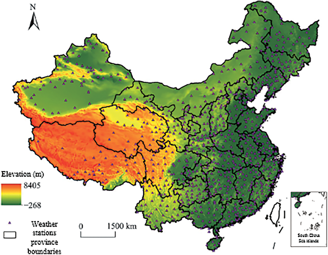
Figure 1: Limits of the focused region, elevations, and meteorological stations
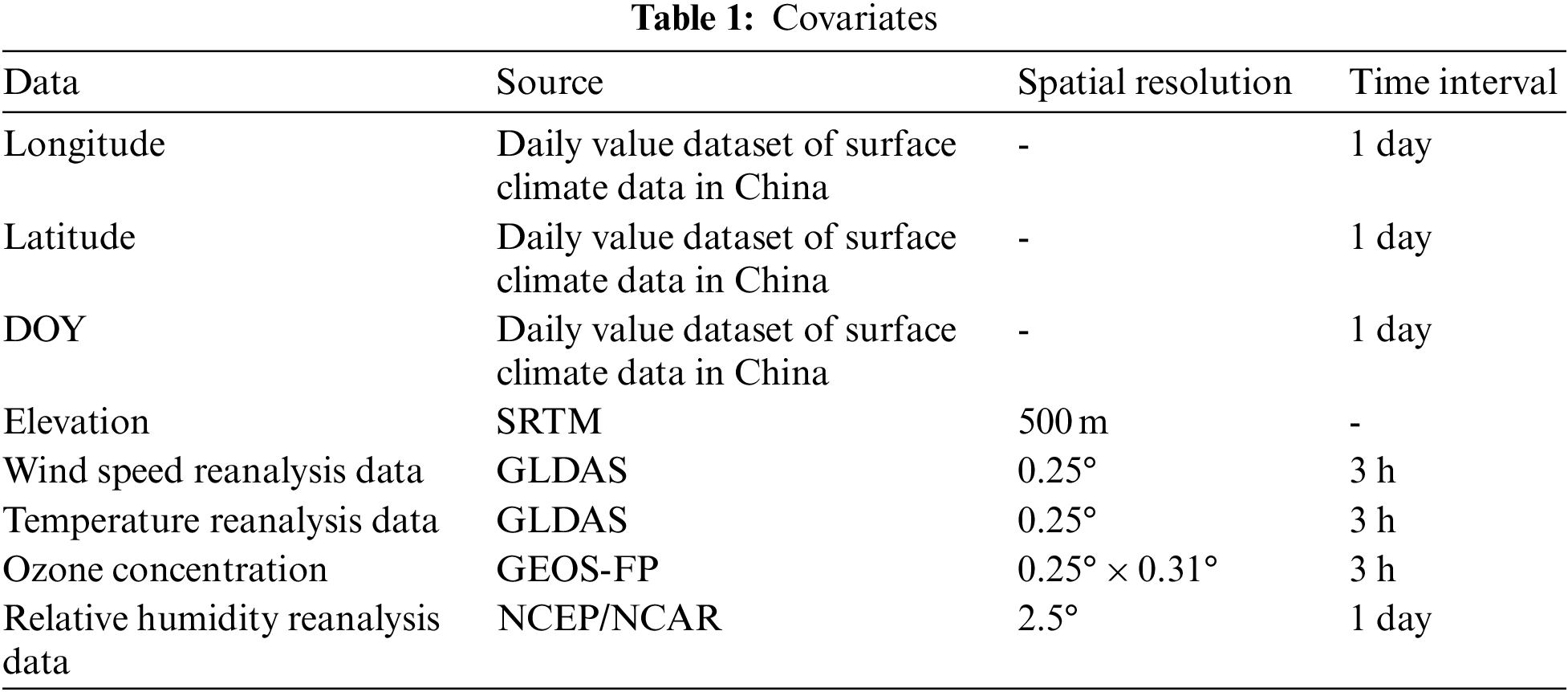
The data used in the study include location information (longitude, latitude) and the day of the year (DOY), which can be used to determine location and time information, as well as explain spatiotemporal variability, which is the basis for meteorological model estimation. The spatialization of air temperature improves model performance with the help of the terrain factor (elevation), which is also used as a covariate in the three meteorological models in this study. According to domain knowledge and exploratory analysis, relative humidity has a certain correlation with ozone concentration [34], temperature and month, and wind speed has a high correlation with gridded wind speed reanalysis data. Therefore, the corresponding covariates were added to the two models respectively.
2.2.1 Ground Meteorological Station Data
The surface meteorological station data comes from the daily value dataset of China’s surface climate data published by the National Meteorological Science Data Sharing Platform (V 3.0), which includes 824 national benchmarks and basic meteorological stations in China. wind speed data. After data filtering, only the values whose quality control is “correct data” is retained. The number of eligible meteorological stations in the temperature, relative humidity and wind speed data in 2015 are 818, 818 and 770, respectively [35–38].
2.2.2 Shuttle Radar Topography Mapping
The elevation data comes from the DEM data with a spatial resolution of 500 m after resampling the Space Shuttle Radar Topographic Mapping (SRTM) mission by the resource and environment data cloud platform. The SRTM is a joint survey completed by National Aeronautics and Space Administration (NASA) and the National Survey and Mapping Agency (NIMA) of the Department of Defense (DoD), as well as the German and Italian space agencies, in February 2000. According to the DEM, which was publicly released in 2003, it covers more than 80% of the earth’s land surface and is available for free.
2.2.3 Global Land Data Assimilation System
The 3-h average wind speed data from the Global Land Data Assimilation System (GLDAS) were used in the construction of the wind speed model. The GLDAS is developed by the Goddard Space Flight Center (GSFC) and the National Environmental Forecaster. The global high-resolution land surface simulation system jointly developed by National Centers for Environmental Prediction (NCEP) can provide global land surface data from 1979 to the present, with a spatial resolution of 0.25° × 0.25° and a time interval of three hours. The GLDAS dataset is freely available from NASA’s Goddard Earth Science Data and Information Service (GES DISC). In addition, GLDAS also provided reanalysis data of wind speed and air temperature for verification of model results [39,40].
2.2.4 Goddard Earth Observation System-Forward Processing
The ozone concentration variable was used in the modeling of relative humidity, and the data were obtained from Goddard Earth Observing System-Forward Processing (GEOS-FP). The GEOS-FP is the latest GEOS-5 meteorological data product produced by the GEOS Data Assimilation System (DAS). The GEOS-FP data can cover the whole of China, the spatial resolution of the data is 0.25° (latitude) × 0.3125° (longitude), and the time interval is three hours (https://ftp://rain.ucis.dal.ca/ctm/GEOS_0.25x0.3125_CH.d/GEOS_FP).
NCEP/NCAR is a joint product of the National Centers for Environmental Prediction (NCEP) and the National Centers for Atmospheric Research (NCAR). The study used the relative humidity reanalysis data it contained to verify the reliability of the relative humidity model results.
See Tab. 1 for a description of the sources of the above covariates and other information.
The study builds models for three meteorological factors respectively, so there are three sets of data.
The air temperature, relative humidity and wind speed models all use longitude, latitude, elevation and DOY as covariates. In addition, the covariates of the relative humidity model are the daily average temperature, the daily average ozone concentration and the nearest neighbor value (the nearest neighbor value refers to the daily average relative humidity value of a station closest to the current point, such as the station closest to point a. is station b, then the nearest neighbor value of point a on a certain day is the value of station b on this day, where the daily average temperature comes from the daily average temperature data generated in this study, the daily average ozone concentration comes from GEOS-FP, and the nearest neighbor value is calculated using python’s SciPy package (the calculation method is kd tree, kd tree is a binary tree with each node as a k-dimensional point, which can be applied to nearest neighbor search, and python’s scipy.spatial.cKDTree can be called for calculation, the parameters are two datasets containing point location information). In this study, the model training phase is the actual site dataset, and the model estimation phase is the actual site dataset and the grid point dataset used for estimation. The wind speed model also uses GLDAS wind speed as a covariate. The time interval of GEOS-FP ozone concentration and GLDAS wind speed are both 3 h. The study averaged 8 of three hours in a day to obtain the daily average value. The image data needs to be resampled in R to the resulting meteorological grid before application.
The construction of high-precision and high-performance models is inseparable from explanatory variables that are significantly related to the explained variables. In this study, the Pearson correlation coefficient between the explained variable and the explanatory variable was calculated to preliminarily judge the possible contribution of the explanatory variable.
3.2 Generalized Additive Model (GAM)
GAM is a generalized nonlinear model (GLM) in which predictors linearly depend on unknown smooth functions of some predictors. This model associates a single response variable Y with some predictor variables xi, Y is specified as an exponential family distribution (such as normal, binomial, and Poisson distribution), and the connection function g (such as identity function and log function) is obtained by Eq. (1) to associate the expectation of Y with these predictors:
Nonparametric means estimation. Its nonparametric form makes the model very flexible, revealing the nonlinear effects of the model. Use the mgcv package in R to build a GAM model for air temperature, relative humidity and wind speed. The formulae of the nonlinear GAM model are as follows:
In the formula: t represents time; s stands for position;
3.3.1 Fully Connected Feedforward Neural Network
A neural network refers to a series of mathematical models inspired by biology and neurology. A fully connected feedforward neural network is a neural network in which the neurons in each layer of the network are connected to the neurons in the next layer. Different network structures are used for different problems. The determination of a network structure needs to specify the number of layers of the network, the number of neurons in each layer and the activation function. The determination of the network structure is equivalent to the determination of the model. Like most machine learning processes, the loss function needs to be specified after the model is determined. Training objective, specifying the optimization algorithm as the training method.
Autoencoder is a kind of feedforward network, which is a kind of neural network with symmetric structure. The number of input variables and output variables is the same, and it can be divided into two stages: encoding and decoding.
Assuming a d-dimensional space input, output x, weight matrix W, bias vector b, parameter set θ, index L of the number of network layers, and map the input to the output, this paper can get the following:
Parameters W, b are obtained by minimizing the L loss between x and xo on the training data:
The autoencoder provides a balanced network topology, and realizes the variable transformation function similar to the principal component analysis in the mapping process from encoding to decoding, and the same output type as the input is similar to adding a regularization factor, which can effectively prevent overfitting.
3.3.3 Residual Network Model Based on Autoencoder
Residual deep network model is a deep learning model mainly used for multiple regression prediction proposed in this paper. The model is derived from the autoencoder by adding residual connections realizes the high-speed transmission of error information, which effectively makes up for the problem that the accuracy of conventional deep networks decreases with the deepening of the number of network layers.
The autoencoder is the fundamental component for implementing residual deep networks. The autoencoder has a mirrored network of encoding and decoding layers. For the coding layer, each hidden layer may have a different number of nodes, these nodes can ensure the change of network variables, and play a role in the compression or adjustment of the network dimension. For the decoding layer, each layer corresponds to the encoding layer (with the same number of layer nodes), and the two correspond to each other to realize the residual connection. For residual regression networks, autoencoders are a natural choice because residual connections typically require two (shallow and deep) to achieve the same number of nodes for direct connections between them. In the previous research of this paper, the residual deep network has greatly improved the prediction accuracy and convergence speed.
The wind speed model and the air temperature model in this study have the same network structure: 5-layer neural network, the number of neurons in each layer is 196, 128, 96, 64 and 32 respectively. The relative humidity model has a 5-layer neural network, and the number of neurons in each layer is 256, 128, 96, 64, and 32, respectively. All three models use the Rectified Linear Unit (Re-LU) function as the activation function of the network, the Mean Square Error (MSE) as the loss function, and the Adaptive Moment Estimation (Adam) as an optimizer.
3.4 Model Accuracy Verification Method
The indicators used in this study to measure the performance of the model are Coefficient of Determination (R2), Root Mean Square Error (RMSE) and Mean Absolute Error (MAE). The coefficient of determination is used to measure the proportion of the variation of the dependent variable that can be explained by the independent variable, so as to judge the explanatory power of the statistical model. The root mean square error can be used to measure the deviation between the estimated value of the model and the observed value. The mean absolute error can better reflect the actual situation of the predicted value error. The specific calculation formula is:
In the formula:
In this paper, the data is divided into three and seven parts, seven parts are used as training data and three parts are used as test data. In addition, in order to detect the overfitting of the model, this paper divides the data set into 10 parts, 9 of which are used for training and 1 for testing in turn, and the result of 10 times of training is ten-fold cross-validation. In this paper, the coefficient of determination (CV R2), root mean square error (CV RMSE) and mean absolute error (CV MAE) of 10-fold cross-validation were calculated.
Ordinary kriging is a commonly used interpolation method in the spatialization of meteorological data. In order to further verify the superiority of the residual model, this paper also performs ordinary kriging interpolation for the three meteorological factors respectively, and calculates the 10-fold cross-validation. R2, RMSE and MAE. In order to verify the reliability of the model results, the Pearson correlation coefficients of the residual model results and the reanalysis data with the measured data at the site were also calculated.
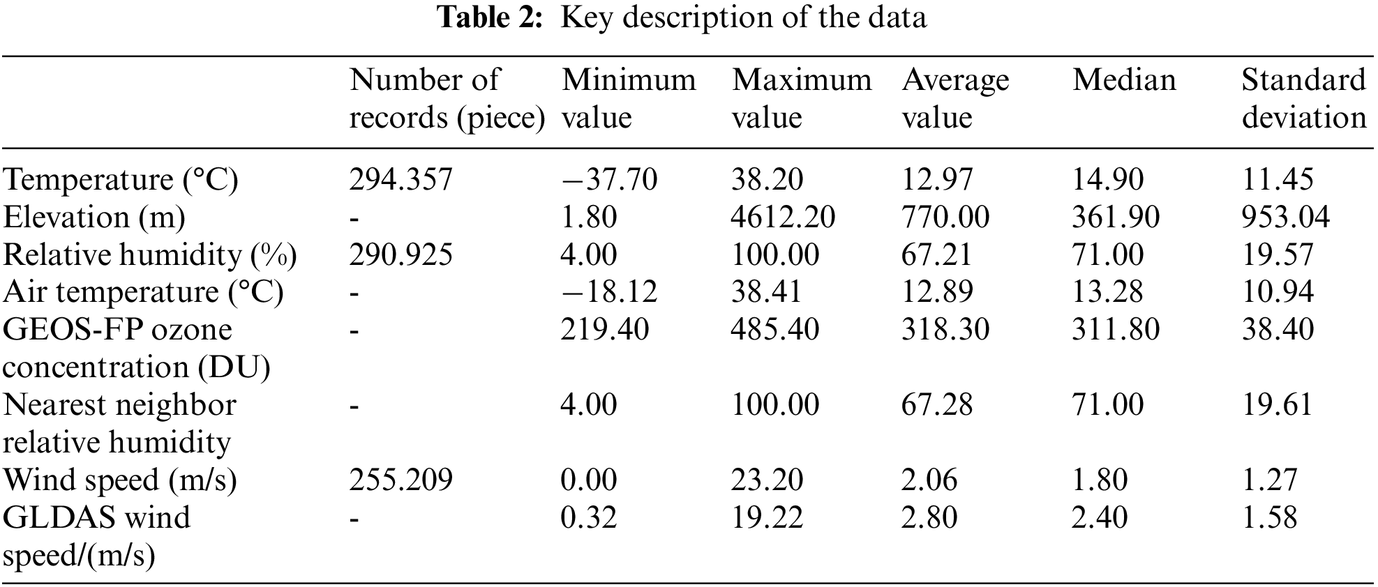
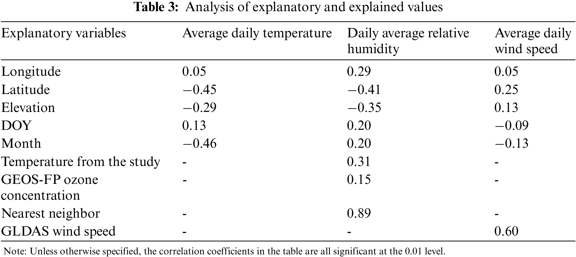
Tab. 2 is the basic statistical information of the three meteorological data. Tab. 3 shows the results of the Pearson correlation analysis between the explained variables and the explanatory variables, and the correlation between the daily average temperature and the latitude is the largest. The daily average relative humidity has the largest correlation with the nearest neighbor value, and also has a great correlation with the same latitude. The correlation coefficient between average daily wind speed and GLDAS wind speed is the largest.
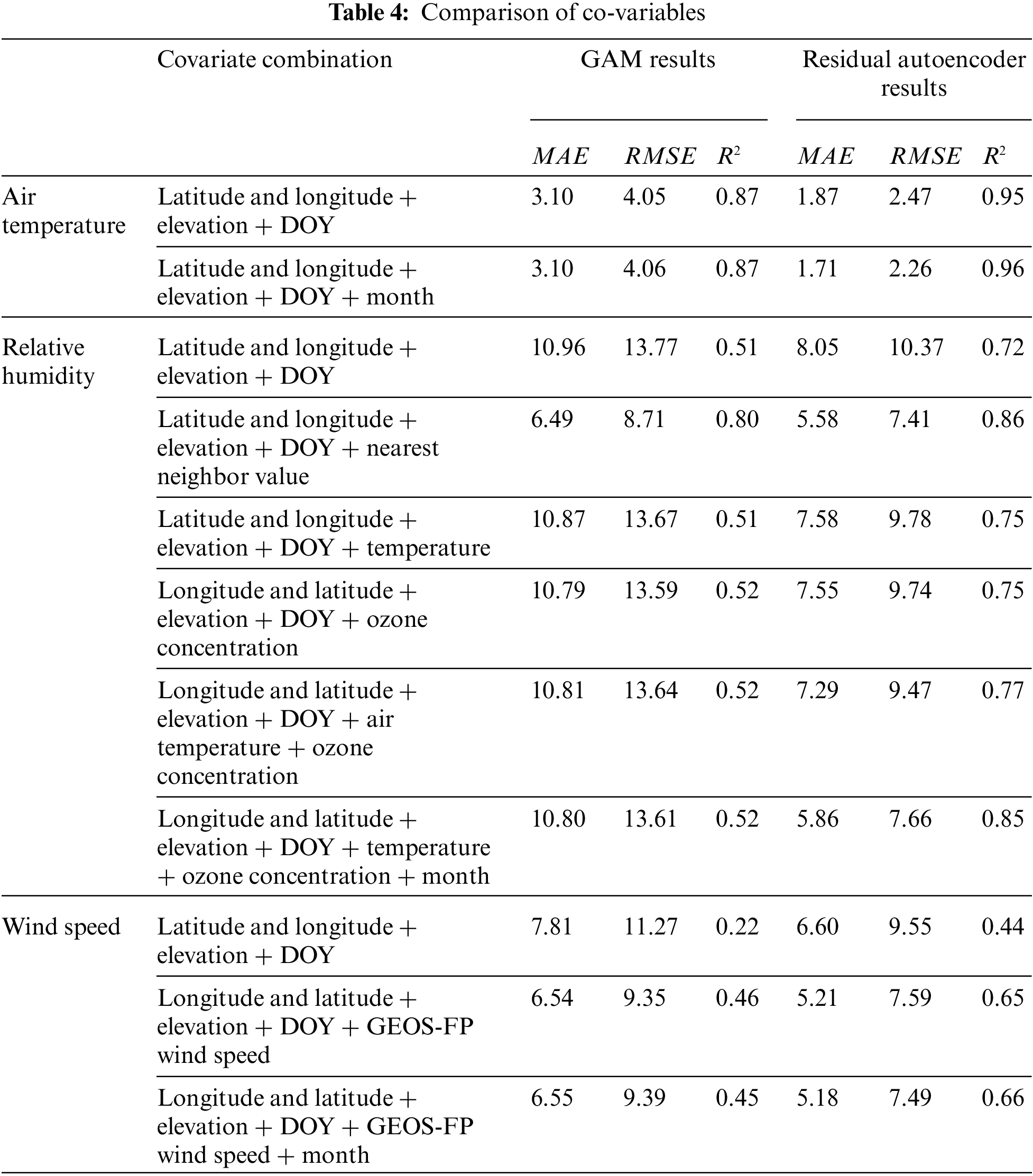
Tab. 4 is the results of the models constructed under different combinations of covariates. The temperature model lists two groups of covariates. The second group adds month on the basis of the first group. Whether it is the GAM method or the residual network method, the improvement of the model after adding the month is not obvious. The study chooses the first group of covariates. Variables participate in model building. The relative humidity model has 6 sets of covariates. For the GAM method, except for the nearest neighbor value, other variables have little help to improve the model. For the residual network, the temperature and ozone concentration can improve the model to a small extent, and the addition of months can greatly improve the accuracy of the model. The study selects the sixth group of covariates to participate in the model construction. The wind speed model has three sets of covariates. The addition of GLDAS wind speed greatly improves the accuracy of the model, while the month has little contribution to the model. The second set of covariates was selected for this study.
Figs. 2–4 are the training results and CV results of the GAM and residual network for air temperature, relative humidity and wind speed, respectively. There is almost no difference between the CV results and the training results of all models, indicating that these models are not overfitting. The residual network models of the three meteorological data are better than the GAM model, and from the scatter plot, the points estimated by the residual network model are more concentrated near the fitting line than the GAM model. The CV R2, RMSE, and MAE of the GAM model of air temperature are 0.87°C, 4.05°C, 3.10°C, respectively, and the CV R2, RMSE, and MAE of the residual network model are 0.95°C, 2.26°C, 2.26°C, respectively. The CV R2, RMSE, and MAE of the GAM model of relative humidity are 0.52%, 13.59%, and 10.59%, respectively. The CV R2, RMSE, and MAE of the residual network model are 0.85%, 7.53%, and 5.78%, respectively. The CV R2, RMSE, and MAE of the GAM model of wind speed are 0.45, 0.84, 0.65 m/s, respectively. The CV R2, RMSE, and MAE of the residual network model are 0.66, 0.74, and 0.51 m/s, respectively.
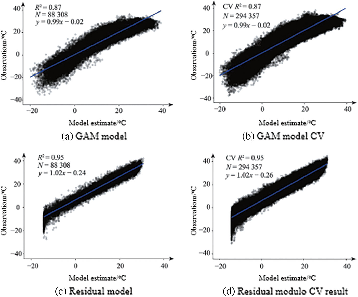
Figure 2: Temperature evaluation
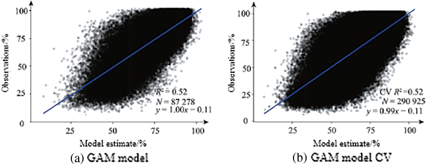
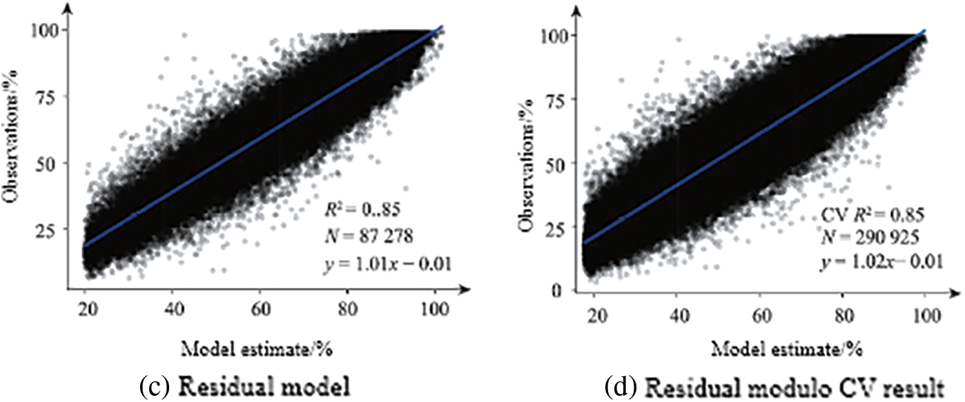
Figure 3: Comparison of relative humidity
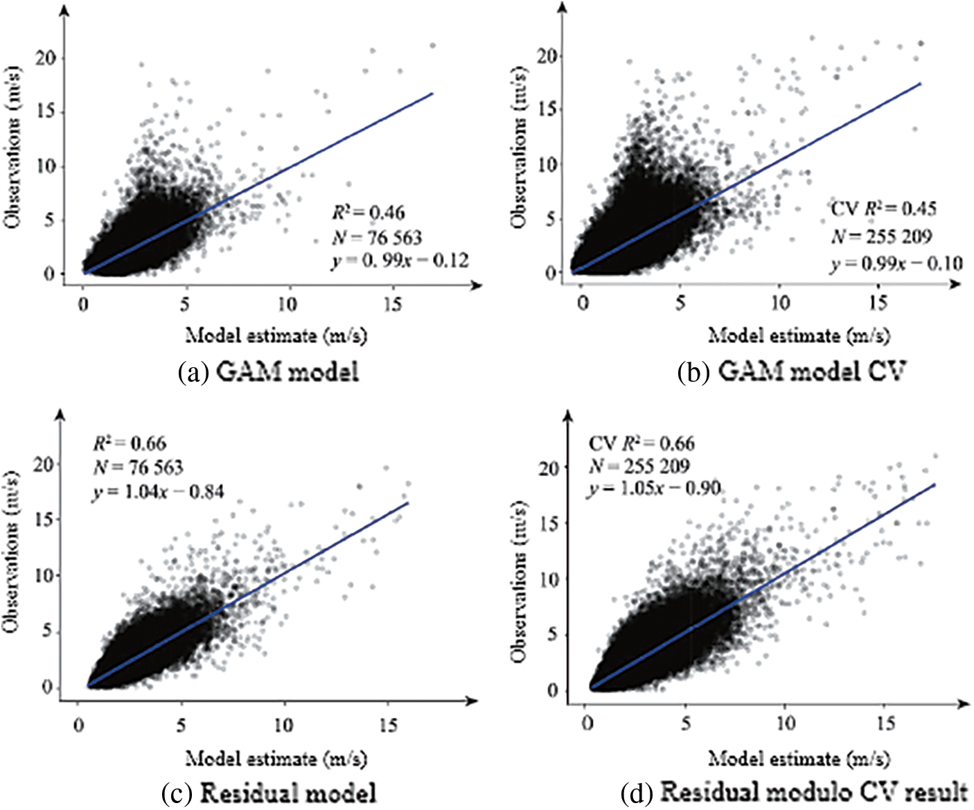
Figure 4: Comparison of wind speed
The study calculated the Pearson correlation coefficients between the observation data of the three meteorological factor stations, the reanalysis data and the residual model results: The correlation coefficients between the observed values of temperature stations and the results of the GLDAS temperature and residual models are 0.96 and 0.97, respectively, which verifies the reliability of the temperature data generated by the residual model. The correlation coefficients between the observed values of wind speed stations and the results of the GLDAS wind speed and residual model are 0.49 and 0.70, respectively, and the results generated by the residual model have better correlation with the observed data of wind speed stations. The correlation coefficients of the relative humidity station observations with the NCEP/NCAR relative humidity and residual model results are 0.50 and 0.74, respectively, indicating that the relative humidity model results in this study are closer to the station measured value.
From the perspective of the model, the GAM model is a nonlinear regression, which is easy to lead to local extreme values in the results, while the residual model is relatively close to the R2 and RMSE of the test due to the application of the symmetric model, and is not prone to overfitting. In terms of meteorological differences, China has a vast territory with large north-south differences. In winter, the temperature is generally low, hot in the south and cold in the north, and the temperature difference between the north and the south is large, exceeding 50°C. In summer, high temperatures are common across the country (except the Qinghai-Tibet Plateau), and the temperature difference between north and south is not large. From the southeast coast to the northwest inland, China can be divided into: Humid, semi-humid, semi-arid, and arid four types of dry and wet areas. The near-surface wind speed in China varies greatly from region to region. In the case of large differences in climate change, it is easier to use a residual model to prevent overfitting, that is, the generation of extreme values. The coordinates and elevations in the model in this study can also capture the underlying surface conditions and terrain conditions well. The results show that the accuracy of the residual model is currently good.
Before and after resampling the image data, the correlation coefficient between the image data value and the explained variable is almost the same (for example, the correlation coefficient of GLDAS wind speed before resampling is 0.59, and the correlation coefficient after resampling is 0.60). The indicators are almost the same (R2, RMSE, MAE). Fig. 5 shows the distribution of the daily average wind speed on January 1, 2015 estimated by the model after the unresampled GLDAS wind speed was used as a covariate and the resampled GLDAS wind speed was used as a covariate to participate in the model construction respectively. Compared with the result after resampling, the result image without resampling is covered with a layer of grid. It is worth noting that this layer of grid and the grid of the GLDAS image overlap, which is called the grid effect. Since the GLDAS image data was used in the estimation of wind speed, and this set of data has some missing values in the coastal and inland areas, the data generated by the study are also missing in the same location.
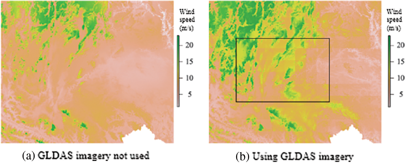
Figure 5: Impact of models of wind speed
4.4 Nearest Neighbor and Raster Polygon Effects
The correlation between the nearest neighbor value and relative humidity is extremely large (the Pearson correlation coefficient is close to 0.9), and at the same time, the model including the nearest neighbor value has a very high explanatory power for the explained variable (CV R2 reaches 0.85). Fig. 6 shows the second covariate (latitude and longitude + elevation + DOY + nearest neighbor value) and the 6th covariate (latitude and longitude + elevation + DOY + air temperature + ozone concentration + month) using the residual network model combined with relative humidity in 2015. Daily average relative humidity distribution map generated on January 1. Comparing the distribution map of daily average relative humidity estimated by the model without using the nearest neighbor value as a covariate, the distribution map using the nearest neighbor value has an obvious polygon mask overlaid on the grid, which is called the polygon effect. The nearest neighbor value as a covariate is the cause of the polygon effect. If the polygon effect caused by the nearest neighbor value can be handled well, then the nearest neighbor value will become a strong predictor.
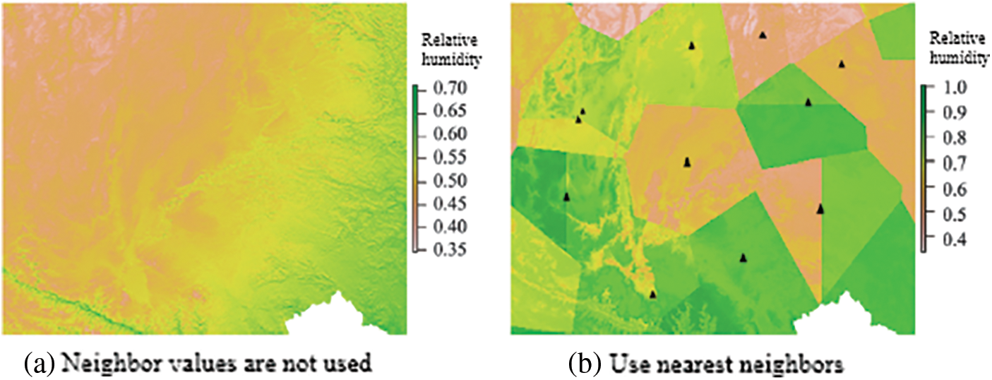
Figure 6: Relative humidity evaluation
4.5 Daily Meteorological Raster Map
The R software was used to generate grid point data at 1 km intervals covering the study area in 2015 (365 days), the covariates required by each model were extracted, and the trained model was used to estimate the value of each meteorological data for each day. Figs. 7–9 are the distributions of daily average temperature, daily average relative humidity and daily average wind speed on January 1, 2015.
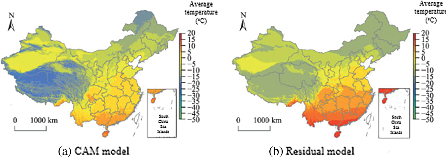
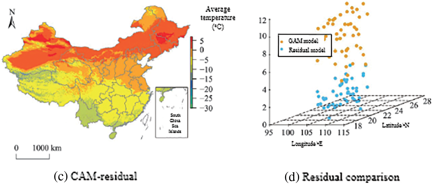
Figure 7: Comparison of average temperature
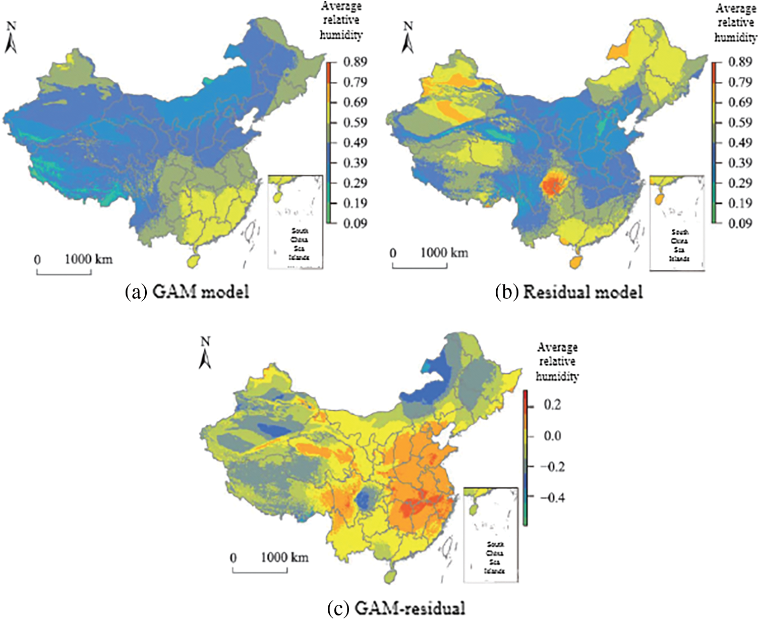
Figure 8: Comparison of average relative humidity
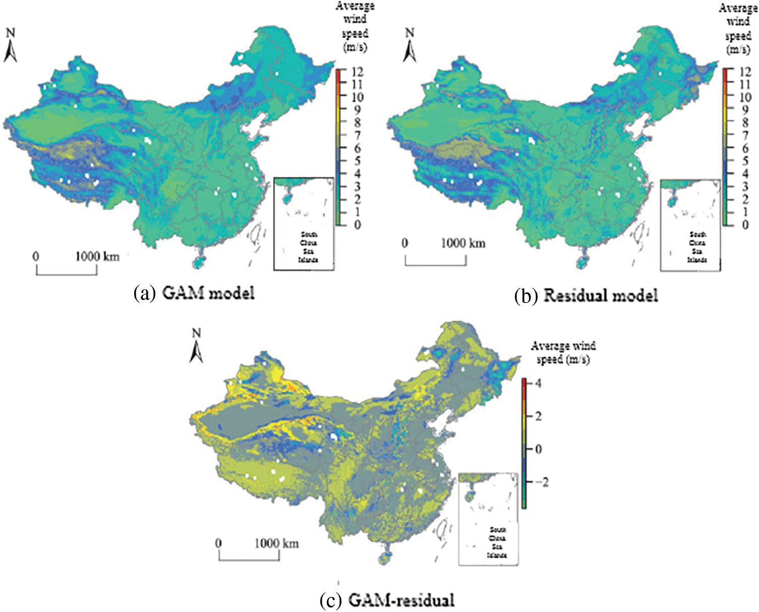
Figure 9: Comparison of average wind speed
In the temperature distribution map of the residual network model in Fig. 7, a clearer temperature boundary can be seen, while the boundary of the distribution map generated by the GAM model is more blurred. Fig. 8c shows the results of the GAM model and the residual network model. The difference between the results, the estimated results of the GAM model are generally lower than those of the residual network model. The study selected sites with a difference of more than 8°C between the results of the two models (the absolute value of the difference between the model result and the observed value), the gap between the GAM result and the observed value is generally large, which proves that the residual model is closer to the true value than the GAM model.
The GAM model has low estimated values in Yunnan, Hainan and other southern regions of China with high temperature values and in the western regions with low temperature values, that is, the estimation ability of the GAM method in extreme value regions is poor, and the estimated values are low. Observing the relative humidity distribution map and the wind speed distribution map, the results of the residual network model show more detailed information.
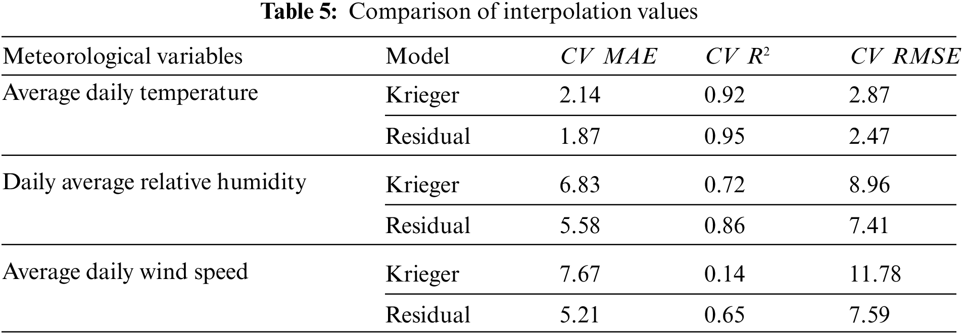
4.6 Ordinary Kriging Method Comparison
In order to compare with traditional meteorological data spatialization methods, the study uses Ordinary Kriging (OK) to interpolate the daily average temperature, daily average relative humidity and daily average wind speed on January 1, 2015, with a 10-fold crossover. The verification results are shown in Tab. 5. The gap between the models increases with the difficulty of variable estimation. For daily average temperature and daily average relative humidity, the results of ordinary kriging are worse than the residual model, but the gap is not large. So obvious, and for the wind speed, the residual model is much better than the ordinary kriging, the CV R2 of the model increases by 0.51, and the CV RMSE and CV MAE decrease by 36% and 32%, respectively. In addition to the advantages in accuracy, the residual model only needs to train a model, and the weather data for a whole year can be estimated by using days as a parameter, while ordinary Kriging interpolation needs to build a model for each day’s data, which is less efficient. In addition, the residual network model is much faster than ordinary kriging interpolation in grid estimation.
The residual network model is used in this paper for high-resolution spatiotemporal estimation of meteorological factors (temperature, relative humidity, and wind speed), and the results outperform the classical nonlinear regression model GAM and the traditional interpolation model ordinary kriging, particularly for relative humidity and wind speed prediction. This paper incorporates spatiotemporal factors into the model, and the results show that the model effectively captures the spatiotemporal changes of each element and achieves better estimation accuracy. For the consideration of temporal correlation, since there are more than 800 ground samples in this paper, the number of samples is limited and the temporal correlation of each sample is different, so it is not suitable to use a time series network similar to Long-Short-Term Memory (LSTM) deep learning models. The residual model used in the study, although it is not the best method to capture the temporal correlation directly with the day as the time element, it can also reflect the influence of the adjacent time sample points on the target point, the day is similar to the weight factor, the most recent (in time) influence of the point is the largest, and the effect is better than other methods in the prediction of the three meteorological factors. In addition, the residuals are randomly distributed, indicating that the model captures major temporal correlations.
Air temperature is a relatively easy-to-interpret variable, and once the geographic location, elevation, and DOY are determined, a good model can be fitted using simple nonlinear regression. When the residual network method is used, the performance of the model is further improved, and both RMSE and MAE are nearly doubled compared with GAM.
The spatial and temporal variability of relative humidity is greater, and it is more difficult to construct a good model and estimate accurately. After the improvement of the model itself encounters a bottleneck, add some relevant variables to improve the table of the model. The current force is a common idea. The addition of the daily average temperature and ozone concentration makes the model improve to a certain extent. Surprisingly, the addition of the month factor makes the R2 of the model increase considerably (0.77∼0.85). This phenomenon did not occur in the air temperature and wind speed models, suggesting the importance of a suitable time factor for the model. In fact, the nearest neighbor value can provide a great contribution to the model, but the addition of the nearest neighbor value also brings the polygon effect of the result grid. In the future research, we will try to use the nearest neighbor value without introducing the polygon effect. Wind speed is the most difficult variable to estimate among the three meteorological factors. There is a high correlation between GLDAS wind speed and site wind speed, and participation in model construction can improve the performance of the model. It should be noted that the image needs to be resampled before using it, otherwise the resulting raster will have a grid effect. GLDAS images have some missing values in coastal areas and land in China, which makes the final data also missing. In the future, this paper hopes to find surrogate covariates for wind speed reanalysis data, in order to generate data products without missing data while ensuring model accuracy. In addition, the wind speed model also considers the nearest neighbor value, but the model accuracy is basically not improved after adding the nearest neighbor value.
The explained variable y is determined by two aspects: the explanatory variable x and the link function f between y and x. When the population has Spatial Stratified Heterogeneity (SSH) and f does not take SSH into account, the estimates based on data learning will be confounding. China covers a large area, and the factors affecting meteorological variables are complex and diverse. In order to further improve the performance of the model, it is possible to test the SSH before determining how to use the model, whether to use it globally or hierarchically. In future research, the geographic detector proposed by [36–38] can be used to detect the presence of SSH in the population. If SSH is not significant, the global statistical model is applicable. If SSH is present, the model can be used separately at each layer to avoid confounding in estimates.
The results of this study provide an important method reference for the high-resolution spatiotemporal estimation of meteorological factors (air temperature, relative humidity and wind speed). With the extension of the method in this paper, generating grid surface results covering meteorological factors across the country can provide an important data source for a variety of applications.
Acknowledgement: The author would like to thanks the editors and reviewers for their review and recommendations.
Funding Statement: The author received no specific funding for this study.
Conflicts of Interest: The authors declare that they have no conflicts of interest to report regarding the present study.
1. Y. Shi, C. Ho and Y. Xu, “Improving satellite aerosol optical depth-PM2.5 correlations using land use regression with microscale geographic predictors in a high-density urban context,” Atmospheric Environment Journal, vol. 190, no. 3, pp. 23–34, 2018. [Google Scholar]
2. E. Aruffo, P. Carlo, P. Cristofanelli and P. Bonasoni, “Neural network model analysis for investigation of NO origin in a high mountain site,” Atmosphere, vol. 11, no. 2, pp. 1–19, 2020. [Google Scholar]
3. X. Ren, Z. Mi and P. Georgopoulos, “Comparison of machine learning and land use regression for fine scale spatiotemporal estimation of ambient air pollution: Modeling ozone concentrations across the contiguous United States,” Environment International Journal, vol. 142, no. 7, pp. 8920–8931, 2020. [Google Scholar]
4. C. Zhang, J. Liu, T. Dong, E. Pattey, J. Shang et al., “Coupling hyperspectral remote sensing data with a crop model to study winter wheat water demand,” Remote Sensing, vol. 11, no. 14, pp. 1–24, 2019. [Google Scholar]
5. V. Rossi, G. Sperandio, T. Caffi, A. Simonetto and G. Gilioli, “Critical success factors for the adoption of decision tool in IPM,” Agronomy, vol. 9, no. 11, pp. 1–17, 2019. [Google Scholar]
6. T. Zhang, Z. Zhang, Y. Li and K. He, “The effects of saline stress on the growth of two shrub species in the qaidam basin of northwestern China,” Sustainability, vol. 11, no. 3, pp. 1–18, 2019. [Google Scholar]
7. C. Bo, H. Song and J. Wang, “Using an autologistic regression model to identify spatial risk factors and spatial risk patterns of hand, foot and mouth disease (HFMD) in mainland China,” BMC Public Health, vol. 14, no. 1, pp. 475–483, 2014. [Google Scholar]
8. Z. Chen, W. Li, J. Guo, Z. Bao and Z. Pan, “Projection of wind energy potential over northern China using a regional climate model,” Sustainability, vol. 12, no. 10, pp. 1–18, 2020. [Google Scholar]
9. Y. Gao, S. Ma, T. Wang, W. Tongliang, Y. Gong et al., “Assessing the wind energy potential of China in considering its variability/intermittency,” Energy Conversion and Management, vol. 226, no. 8, pp. 1183–1194, 2020. [Google Scholar]
10. W. Liu, Q. Zhang, Z. Fu, X. Chen and H. Li, “Analysis and estimation of geographical and topographic influencing factors for precipitation distribution over complex terrains: A case study of the northeast slope of the qinghai-Tibet plateu,” Atmosphere Journal, vol. 9, no. 9, pp. 1–18, 2018. [Google Scholar]
11. R. Yang and B. Xing, “A comparison of the performance of different interpolation methods in replicating rainfall magnitudes under different climatic conditions in Chongqing province,” Atmosphere Journal, vol. 12, no. 10, pp. 1–15, 2021. [Google Scholar]
12. S. Chen and J. Guo, “Spatial interpolation techniques: Their applications in regionalizing climate-change series and associated accuracy evaluation in northeast China,” Geomatics, Natural Hazards and Risk, vol. 8, no. 2, pp. 689–705, 2016. [Google Scholar]
13. B. Zhang and W. Zhou, “Spatial-temporal characteristics of precipitation and its relationship with land use/cover change on the Qinghai-tibet plateu, China,” Land Journal, vol. 10, no. 3, pp. 1–18, 2021. [Google Scholar]
14. W. Xu, Y. Zou, G. Zhang and M. Linderman, “A comparison among spatial interpolation techniques for daily rainfall data in Sichuan province,” International Journal of Climatology, vol. 35, no. 10, pp. 2898–2907, 2015. [Google Scholar]
15. K. Fung, K. Chew, Y. Huang, A. Ahmed, F. Yenn et al., “Evaluation of spatial interpolation methods and spatiotemporal modeling of rainfall distribution in paninsular Malaysia,” Ain Shams Engineering Journal, vol. 13, no. 2, pp. 3972–3983, 2022. [Google Scholar]
16. M. Wang, G. He, Z. Zhang, G. Wang, Z. Zhang et al., “Comparison of spatial interpolation and regression analysis models for an estimation of monthly near surface air temperature in China,” Remote Sensing, vol. 9, no. 12, pp. 1–32, 2017. [Google Scholar]
17. C. Berndt and U. Haberlandt, “Spatial interpolation of climate variables in northern Germany–influence of temporal resolution and network density,” Journal of Hydrology: Regional Studies, vol. 15, no. 5, pp. 184–202, 2018. [Google Scholar]
18. D. Zou, W. Hou, H. Wu, P. Yan and Q. Zhang, “Feasibility of calculating standardized precipitation index with short-term precipitation data in China,” Atmosphere Journal, vol. 12, no. 5, pp. 1–23, 2021. [Google Scholar]
19. D. Xu, J. Wang and Q. Li, “A new method for temperature spatial interpolation based on sparse historical stations,” Journal of Climate, vol. 31, no. 5, pp. 1757–1770, 2017. [Google Scholar]
20. J. Wang, C. Xu and M. Hu, “Global land surface air temperature dynamics since 1880,” International Journal of Climatology, vol. 381, no. 5, pp. 466–474, 2018. [Google Scholar]
21. J. Wang, C. Xu and M. Hu, “A new estimate of the China temperature anomaly series and uncertainty assessment in 1900–2006,” Journal of Geophysical Research: Atmosphere¸, vol. 119, no. 1, pp. 1–9, 2014. [Google Scholar]
22. G. Pellicone, T. Caloiero, G. Modica and I. Guagliardi, “Application of several spatial interpolation techniques to monthly rainfall data in the Calabria region (southern Italy),” International Journal of Climatology, vol. 38, no. 9, pp. 3651–3666, 2018. [Google Scholar]
23. Y. Cui, C. Pan, C. Liu, M. Luo and Y. Guo, “Spatiotemporal variation and tendency analysis on rainfall erosivity in the loess plateu of China,” Hydrology Research, vol. 51, no. 5, pp. 1048–1062, 2020. [Google Scholar]
24. Y. Sun, Q. Guan, Q. Wang, L. Yang, N. Pan et al., “Quantitative assessment of the impact of climatic factors on phenological changes in the qilian mountains, China,” Forest Ecology and Management¸ vol. 499, no. 5, pp. 1199–1208, 2021. [Google Scholar]
25. D. Cho, C. Yoo, J. Im, Y. Lee and J. Lee, “Improvement of spatial interpolation accuracy of daily maximum air temperature in urban areas using a stacking ensemble technique,” GISscience & Remote Sensing, vol. 57, no. 5, pp. 633–649, 2020. [Google Scholar]
26. T. Appelhans, E. Mwangomo, D. Hardy, A. Hemp and T. Nauss, “Evaluating machine learning approaches for the interpolation of monthly air temperature at mt. Kilimanjaro, Tanzania,” Spatial Statistics Journal, vol. 14, no. 1, pp. 91–113, 2015. [Google Scholar]
27. Z. Lv, X. Liu, W. Cao and Y. Zhu, “A model-based estimate of regional wheat yield gaps and water use efficiency in main winter wheat production regions of China,” Scientific Reports, vol. 7, pp. 1–19, 2017. [Google Scholar]
28. G. Mamadjanova and G. Leckebusch, “Assessment of mudflow risk in Uzbekistan using CMIP5 models,” Weather and Climate Extremes, vol. 36, no. 2, pp. 3375–3384, 2022. [Google Scholar]
29. J. Lazzus, “Estimation of surface soil temperature based on neural network modeling,” Italian Journal of Agrometeorology, vol. 19, no. 2, pp. 5–12, 2014. [Google Scholar]
30. M. Szymanowski, M. Kryza and W. Spallek, “Regression-based air temperature spatial prediction models: An example from Poland,” Meteorologische Zeitschirift, vol. 22, no. 5, pp. 577–585, 2013. [Google Scholar]
31. J. Hjort, J. Suomi and J. Kayhko, “Spatial prediction of urban-rural temperatures using statistical methods,” Theoretical and Applied Climatology, vol. 106, no. 1, pp. 139–152, 2011. [Google Scholar]
32. X. Kou, L. Jiang and Y. Bo, “Estimation of land surface temperature through blending MODIS and AMSR-E data with the Bayesian maximum entropy method,” Remote Sensing Journal, vol. 8, no. 2, pp. 1–27, 2016. [Google Scholar]
33. X. Wang, B. Chu, X. Feng, Y. Li, B. Fu et al., “Spatiotemporal variation and driving factors of water yield services on the qingzang plateu,” Geography and Sustainability, vol. 2, no. 1, pp. 31–39, 2021. [Google Scholar]
34. C. Lin, A. Lau, J. Fung, Y. Song, Y. Li et al., “Removing the effects of meteorological factors on changes in nitrogen dioxide and ozone concentrations in China from 2013 to 2020,” Science of the Total Environment, vol. 793, no. 8, pp. 4521–4533, 2021. [Google Scholar]
35. A. Navamuel, F. Magalhaes, D. Sanchez, J. Angel, D. Sanchez et al., “Deep learning enhanced principle component analysis for structural health monitoring,” Structural Health Monitoring Journal¸, vol. 1, no. 2, pp. 872–883, 2022. [Google Scholar]
36. J. Wang, T. Zhang and B. Fu, “A measure of spatial stratified heterogeneity,” Ecological Indicators, vol. 67, no. 3, pp. 250–256, 2016. [Google Scholar]
37. X. Deng, Y. Liu, F. Gao, S. Liao, F. Zhou et al., “Spatial distribution and mechanism of urban occupation mixture in Guangzhou: An optimized geodetector-based index to compare individual and interactive effects,” International Journal of Geo-Information, vol. 10, no. 10, pp. 1–19, 2021. [Google Scholar]
38. J. Wang, X. Li and G. Christakos, “Geographical detectors-based health risk assessment and its application in the neural tube defects study of the heshun region, China,” International Journal of Geographical Information Science, vol. 24, no. 1, pp. 107–127, 2010. [Google Scholar]
39. R. Zhang, W. F. Zhang, W. Sun, X. M. Sun and S. J. Jha, “A robust 3-D medical watermarking based on wavelet transform for data protection,” Computer Systems Science & Engineering, vol. 41, no. 3, pp. 1043–1056, 2022. [Google Scholar]
40. R. Zhang, X. Sun, X. M. Sun and S. K. Jha, “Robust reversible audio watermarking scheme for telemedicine and privacy protection,” Computers, Materials & Continua, vol. 71, no. 2, pp. 3035–3050, 2022. [Google Scholar]
 | This work is licensed under a Creative Commons Attribution 4.0 International License, which permits unrestricted use, distribution, and reproduction in any medium, provided the original work is properly cited. |