Computers, Materials & Continua DOI:10.32604/cmc.2022.028441
Article

Design and Implementation of a State-feedback Controller Using LQR Technique

Aamir Shahzad1,*, Shadi Munshi2, Sufyan Azam2 and Muhammad Nasir Khan3

1Mechanical Engineering Department, The University of Lahore, Lahore, Pakistan
2Mechanical Engineering Department, Umm Al-Qura University, Makkah, Saudi Arabia
3Electrical Engineering Department, The University of Lahore, Lahore, Pakistan
*Corresponding Author: Aamir Shahzad. Email: aamir.shahzad1@me.uol.edu.pk
Received: 10 February 2022; Accepted: 01 April 2022

Abstract: The main objective of this research is to design a state-feedback controller for the rotary inverted pendulum module utilizing the linear quadratic regulator (LQR) technique. The controller maintains the pendulum in the inverted (upright) position and is robust enough to reject external disturbance to maintain its stability. The research work involves three major contributions: mathematical modeling, simulation, and real-time implementation. To design a controller, mathematical modeling has been done by employing the Newton-Euler, Lagrange method. The resulting model was nonlinear so linearization was required, which has been done around a working point. For the estimation of the controller parameters, MATLAB LQR function has been utilized. Simulation has been performed for the designed controller and it also has been implemented and tested over the real inverted pendulum. From the results, it is vivid that the designed controller keeps the inverted pendulum in an upright position and rejects the disturbances and falling under gravitational force by adjusting the rotation of the horizontal link.

Keywords: Mathematical modeling; linearization; linear quadratic regulator (LQR); nonlinear system; rotary inverted pendulum

1  Introduction

The rotary inverted pendulum is an important topic of research in control engineering. It is an effective tool to test the performance of different control approaches. It is a multi-variable nonlinear dynamical system that is highly unstable. It has two links, one link revolves around an axis in the horizontal plane so that the other can balance itself in an upright position [1–5]. The control of the rotary inverted pendulum helps in designing the altitude controller of rockets and satellites due to its nonlinear behavior. The inverted pendulum control is playing a vital role in real-life applications ranging from robotics to aerospace, locomotive to marine systems and from flexible to pointing control systems. Additionally, the study of dynamics and control of inverted pendulum helps in maintaining the equilibrium of tall buildings [6–12].

Various efforts have been reported in the literature about the design, mathematical modeling and stable control of inverted pendulum by utilizing different control approaches. Model-based control techniques have been used frequently but the fuzzy and non-model-based approaches have been utilized too. Newton’s laws or energy balance approaches have been used to formulate the dynamic model [13–15]. The fuzzy cascade control based on Hierarchical Fair Competition-based Genetic Algorithms has been used in [16]. It consists of two fuzzy controllers which have been placed in a cascade manner and their parameters have been optimized using the genetic algorithm. The inner loop controls the position of the rotating arm while the outer loop provides the appropriate input to the inner loop due to a change in the angle of the vertical arm. Simulation has been performed and the results have been validated on the real hardware. Counter based approach has been used to design a swing-up controller while pole placement with an integrator has been used to stabilize the vertical arm in [17]. The study shows a settling time of 4.5 s for the swing-up controller. Similarly, stabilization of the vertical arm has been shown through simulation. The actual implementation over the hardware has not been reported.

Swing up and vertical stabilization have been achieved in [18] through the energy-based method. H2/H∞ controller has been used to reduce oscillations and stabilization of the system. Lesser oscillations have been observed with the proposed controller as compared to the state feedback controller. The only drawback is that the control signal is not optimal and requires a higher value for smaller oscillations. In [19], Kharitonov polynomial has been formed with a PI controller. Routh Hurwitz criteria have been utilized to design a stable controller and stability has been analyzed by using the Nyquist plot. A swing-up controller has been designed in [20]. It is based on energy control and feedback linearization. Simulation has been performed to show the effectiveness of the proposed approach. The value of gain has been associated with energy convergence to zero. The higher gain means the faster convergence. Another control approach has been reported in [21]. It consists of a backstepping controller for swing-up and linear state feedback controllers for stabilization. Quadratic Lyapunov approach and Sylvester’s criterion, have been used to determine a sufficient stability margin around the equilibrium point. A comparison has been done between the proposed approach and the classical scheme and results have been evaluated in terms of percentage to show the effectiveness of the proposed approach [21].

Mathematical modeling and simulation of complex and multivariable systems is an active field of research to find an optimal solution through the design and development of new algorithms. It is a cost-effective process that provides an insight into the robustness and suitability of an algorithm for a particular problem to be solved. It sheds light on the possible outcomes and helps in analysis through variation of system parameters [22–37]. Therefore, it was necessary to develop a complete model of the rotary inverted pendulum, its parameters estimation and testing over real hardware to validate the results found in the simulation. To the best of our knowledge, no such design of controller with linearization and analysis has been done so far. This paper describes the two-link inverted pendulum. In the proposed research work, the following are the key developments contributions:

•   To design the controller, complete mathematical modeling has been done using the Newton-Euler, Lagrange approach

•   The non-linear model has been linearized around a working point

•   Feedback gains of linear quadratic regulator (LQR) controller have been evaluated using MATLAB (2018a, MathWorks, MA, USA)

•   The designed controller performance has been tested in a simulation environment as well as it has been implemented over an inverted pendulum. It shows that the controller keeps the pendulum in the upright position and rejects the disturbances

The paper has been organized as follows. Section I is Introduction. In Section II, mathematical modeling has been developed and linearization has been done around the working point. Simulation results have been presented in Section III. Implementation over a real rotary inverted pendulum has been done in Section IV. Section V has the conclusion and future work.

2  System Modeling

A free-body diagram of the pendulum with reference frames is shown in Fig. 1. It is vivid from Fig. 1, that the horizontal link having a length r is rotating at an angle θ and the vertical arm having a length L with mass m swings at an angle α. Reference frames are attached to moving links to calculate the position vector with respect to a fixed frame. Tab. 1 shows the symbols used in the derivation of system mathematical modeling.

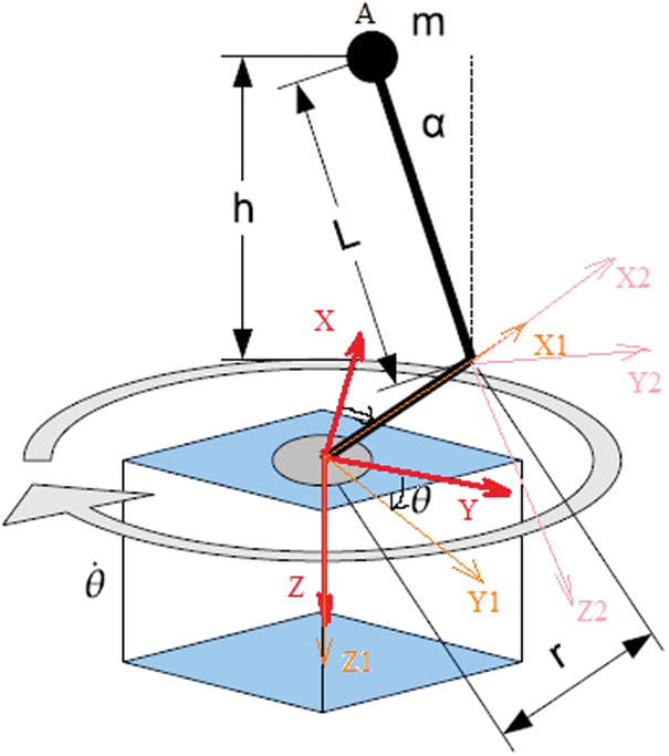
Figure 1: Free body diagram of the pendulum with reference frames

2.1 System Model Development

The potential energy (PE) Epot of the inverted pendulum is given by:

Epot=mgLcos⁡α(1)

where m denotes the mass of the pendulum arm, g is the force of gravity, L is the length of the pendulum’s center of mass and α represents the deflection of the pendulum arm. The kinetic energy (KE) Ekin of the inverted pendulum is given by:

Ekin=mv22+Jeqθ˙22(2)

where v denotes the velocity of mass m, Jeq is the inertia of the pendulum and θ˙ denotes the angular velocity of the horizontal link. In order to evaluate v, a position vector p of mass must be defined as:

p_=[xyz]=[cosθ−sinθ0sinθcosθ0001]([r00]+[1000cosαsinα0−sinαcosα][00−L])(3)

p_=[xyz]=[cosθ−sinθ0sinθcosθ0001][r−Lsinα−Lcosα](4)

p_=[xyz]=[rcosθ+Lsinθsinαrsinθ+Lcosθsinα−Lcosα](5)

where r denotes the length of the horizontal link. To evaluate velocity v_, we need to differentiate the position vector p of m as:

v_=p_=[x˙y˙z˙]=[−rsinθθ˙+Lcosθsinαθ˙+Lsinθcosαα˙−rcosθθ˙+Lsinθsinαθ˙−Lcosθcosαα˙−Lsinαα˙](6)

v2=x˙2+y˙2+z˙2=(−rsinθθ˙+Lcosθsinαθ˙+Lsinθcosαα)˙2+(−rcosθθ˙+Lsinθsinαθ˙−Lcosθcosαα˙)2+(−Lsinαα)˙2 (7)

v2=r2θ˙2+L2sin2αθ˙2+L2cos2αα˙2−2rLcosαθ˙α˙+L2sin2αα˙2(8)

v2=r2θ˙2+L2sin2αθ˙2+L2α˙2−2rLcosαθ˙α˙(9)

Substituting Eq. (9) in Eq. (2), we get:

Ekin=12mr2θ˙2+12mL2sin2⁡αθ˙2+12mL2α˙2−mrLcos⁡αθ˙α˙+Jeqθ˙22(10)

The Lagrangian LLagr is given by:

LLagr=Ekin−Epot(11)

LLagr=12mr2θ˙2+12mL2sin2⁡(α)θ˙2+12mL2α˙2−mrlcos⁡αθ˙α˙+12Jeqθ˙2−mgLcos⁡α(12)

The states of the system (i.e., q∈(q1,q2)) are given by:

q_=[θα](13)

where the working points (q1,q2) are given by:

q_1=[θ∘0],q_2=[θ∘π](14)

Taking the differential of Eq. (12) with respect to θ˙ to get:

δδθ˙[LLagr]=mr2θ˙+mL2sin2⁡αθ˙−mrLcos⁡αα˙+Jeqθ˙(15)

Now taking d/dt of Eq. (15) to get:

ddt(δδθ˙[LLagr])=mr2θ¨+2mL2sin⁡αcos⁡αθ˙α˙+mL2sin2⁡αθ¨+mrLsin⁡αα˙2−mrLcos⁡αα¨+Jeqθ¨(16)

Taking the differential of Eq. (12) with respect to θ to get:

δδθ[LLagr]=0(17)

where:

ddt(δδθ˙[LLagr])−δδθ[LLagr]=T(18)

where T denotes the torque. By inserting Eq. (16) and Eq. (17) in Eq. (18) to get:

mr2θ¨+2mL2sin⁡αcos⁡αθ˙α˙+mL2sin2⁡αθ¨+mrLsin⁡αα˙2−mrLcos⁡αα¨+Jeqθ¨=T(19)

Now differentiating Eq. (12) with respect to α and α˙ respectively to get:

δδα[LLagr]=mL2sin⁡αcos⁡αθ˙2+mrLsin⁡αθ˙α˙+mgLsin⁡α(20)

δδα˙[LLagr]=mL2α˙−mrLcos⁡αθ˙(21)

Now taking d/dt of Eq. (21) to get:

ddt(δδα˙[LLagr])=mL2α¨+mrLsin⁡αθ˙α˙−mrLcos⁡αθ¨(22)

where:

ddt(δδα˙[LLagr])−δδα[LLagr]=0(23)

Now simplify Eq. (23) to get:

mL2α¨−mrLcos⁡αθ¨−mL2sin⁡αcos⁡αθ˙2−mgLsin⁡α=0(24)

Finally, we get two equations (i.e. Eq. (25) and Eq. (26)) of the system as under:

r2θ¨+2L2sin⁡αcos⁡αθ˙α˙+L2sin2⁡αθ¨+rLsin⁡αα˙2−rLcos⁡αα¨+Jeqmθ¨=Tm(25)

Lα¨−rcos⁡αθ¨−Lsin⁡αcos⁡αθ˙2−gsin⁡α=0(26)

From Eq. (26), the value of α¨ is obtained as:

α¨=rLcos⁡αθ¨+sin⁡αcos⁡αθ˙2+gLsin⁡α(27)

Substituting the value of α¨ from Eq. (27) in Eq. (25)

r2θ¨+2L2sin⁡αcos⁡αθ˙α˙+L2sin2⁡αθ¨+rLsin⁡αα˙2−r2cos2⁡αθ¨−rLsin⁡αcos2⁡αθ˙2−rgcos⁡αsin⁡α+Jeqmθ¨=Tm(28)

Now simplifying the Eq. (28):

θ¨[sin2⁡α(L2+r2)+Jeqm]+2L2sin⁡αcos⁡αθ˙α˙+rLsin⁡αα˙2−rLsin⁡αcos2⁡αθ˙2−rgcos⁡αsin⁡α=Tm(29)

θ¨=1sin2⁡α.(L2+r2)+Jeqm[Tm−2L2sin⁡αcos⁡αθ˙α˙−rLsin⁡αα˙2+rLsin⁡αcos2⁡αθ˙2+rgcos⁡αsin⁡α](30)

Substituting the value θ¨ in Eq. (27):

α¨=(rcos⁡αL[sin2⁡α(L2+r2)+Jeqm])[Tm−2L2sin⁡αcos⁡αθ˙α˙−rLsin⁡αα˙2+rLsin⁡αcos2⁡αθ˙2+rgcos⁡αsin⁡α]+sin⁡αcos⁡αθ˙2+gLsin⁡α (31)

2.2 System Linearization

To design the controller, mathematical modeling has been done by employing the Newton-Euler, Lagrange method. The resulting model is nonlinear so linearization is required, which has been done around a working point. Following are the assumptions from Eqs. (30) and (31).

θ¨=f1=(1sin2α(L2+r2)+Jeqm)[Tm−L2sin2αθ˙α˙−rLsinαα˙2+rLsinαcos2αθ˙2+12rgcosαsin2α] (32)

α¨=f2=(rcosαLsin2α(L2+r2)+Jeqm)[Tm−L2sin2αθ˙α˙−rLsinαα˙2+rLsinαcos2αθ˙2+12rgsin2α]+12sin2αθ˙2+gLsinα(33)

The linear system can be expressed by:

x˙_=A_x_+B_u_,y_=C_x_+D_u_(34)

For the nonlinear system, the linearized system looks as:

[θ˙θ¨α˙α¨]=[0100δf1δθx_=xo_δf1δθ˙x_=xo_δf1δαx_=xo_δf1δα˙x_=xo_0001δf2δθx_=xo_δf2δθ˙x_=xo_δf2δαx_=xo_δf2δα˙x_=xo_][θθ˙αα˙]+[0δf1δTx_=xo_0δf2δTx_=xo_]T(35)

[y1y2]=[10000010][θθ˙αα˙](36)

The working point is given by:

xo_=[θo000](37)

δδθ[f1]=0(38)

δδθx_=xo_[f1]=0(39)

δδθ˙[f1]=(1sin2⁡α(L2+r2)+Jeqm)[−L2sin⁡2αα˙+2rLsin⁡αcos2⁡αθ˙](40)

δδθ˙x_=xo_[f1]=0(41)

δδα[f1]=(−2sin⁡αcos⁡α(L2+r2)[sin2⁡α(L2+r2)+Jeqm]2)[Tm−L2sin⁡2αθ˙α˙−rLsin⁡αα˙2+rLsin⁡αcos2⁡αθ˙2+12rgsin⁡2α]+(1sin2⁡α(L2+r2)+Jeqm)[−2L2cos⁡2αθ˙α˙−rLcos⁡αα˙2+rLcos3⁡αθ˙2−2rLsin2⁡αcos⁡αθ˙2+rgcos⁡2α](42)

δδαx_=xo_[f1]=mrgJeq(43)

δδα˙[f1]=(1sin2α(L2+r2)+Jeqm)[−L2sin2αθ˙−rLsinαα˙](44)

δδα˙x_=xo_[f1]=0(45)

δδT[f1]=(1sin2⁡α(L2+r2)+Jeqm)1m(46)

δδTx_=xo_[f1]=1Jeq(47)

δδθ[f2]=0(48)

δδθx_=xo_[f2]=0(49)

δδθ˙[f2]=(rcos⁡αL[sin2⁡α(L2+r2)+Jeqm])[−L2sin⁡2αα˙+2rLsin⁡αcos2⁡αθ˙](50)

δδθ˙x_[f2]=xo_=0(51)

δδα[f2]=(−Lrsin⁡α(sin2⁡α(L2+r2)+Jeqm)[L(sin2⁡α(L2+r2)+Jeqm)]2)−(2Lrsin⁡αcos2⁡α(L2+r2)[L(sin2⁡α(L2+r2)+Jeqm)]2)×[Tm−L2sin2αθ˙α˙−rLsinαα˙2+rLsinαcos2αθ˙2+12rgsin2α]+(rcos⁡αL(sin2⁡α(L2+r2)+Jeqm))[−2L2cos2αθ˙α−˙rLcosαα˙2+rLcos3αθ˙2−2rLsin2αcosαθ˙2+rgcos2α]+cos⁡2αθ˙2+gLcos⁡α(52)

δδαx_=xo_[f2]=mr2gJeqL+gL(53)

δδα˙[f2]=(rcos⁡αL[sin2⁡α(L2+r2)+Jeqm])[−L2sin⁡2αθ˙−2rLsin⁡αα˙](54)

δδα˙x_=xo_[f2]=0(55)

δδT[f2]=(rcos⁡αL[sin2⁡α(L2+r2)+Jeqm])1m(56)

δδTx_=xo_[f2]=rLJeq(57)

The linearized system is given by:

[θ˙θ¨α˙α¨]=[010000mrgJeq0000100gL(1+mr2Jeq)0][θθ˙αα˙]+[01Jeq0rLJeq].T(58)

[y1y2]=[10000010][θθ˙αα˙](59)

The motor torque equation is given by:

T=Tgear−Beqθ˙=KtKgRmηmηg(U−KmKgθ˙)−Beqθ˙=KtKgRmηmηgU−θ˙(KtKg2KmRmηmηg+Beq)(60)

where U is the input voltage and is a control signal. Substitute the value of T in the state-space model and we get:

[θ˙θ¨α˙α¨]=[010000mrgJeq0000100gL(1+mr2Jeq)0][θθ˙αα˙]+[0KtKgηmηgRmJeq0rKtKgηmηgLRmJeq]U−[0a0b].θ˙(61)

where:

a=−1Jeq(KtKg2KmηmηgRm+Beq)

b=−rLJeq(KtKg2KmηmηgRm+Beq)

[θ˙θ¨α˙α¨]=[01000am.r.gJeq000010bgL(1+mr2Jeq)0][θθ˙αα˙]+[0KtKgηmηgRmJeq0rKtKgηmηgLRmJeq]U(62)

where, Beq denotes the viscous damping of the motor, ηg is the efficiency of the gear, ηm represents the efficiency of the motor, Rm is the resistance of the motor, Kt is the torque constant of the motor, Kg is the gear ratio, Km is the damping constant, Kenc is the encoder constant and U is the control voltage.

3  Controller Design and Parameters Estimation

MATLAB (2018a, MathWorks, MA, USA) has been used to evaluate the parameters of the LQR controller. Matrices given in (A) and (B) have been evaluated using the system setup parameters and initial conditions given in Tab. 2. Similarly, the matrix given in (C) has been evaluated using the same set of parameters and MATLAB LQR function.

A=[01000−20.3854.06000010−19.22109.560](A)

B=[035.84033.81](B)

K=[−1−2.0227.683.56](C)

Fig. 2 shows the linearized model of inverted pendulum with LQR controller simulated in MATLAB Simulink module. In order to analyze performance and the stability of the controller, a horizontal link having an angle theta (θ) has been rotated at an angle of 5.7 degrees (i.e., 0.1 radians) after an interval of one second. The vertical arm swings at a certain angle and again come back to zero degrees and stays in an upright position while the horizontal link moves from zero to 5.7 degrees position. The simulation result is showing the stable behavior of the system as shown in Fig. 3. This proves that the system is stable and the controller keeps the pendulum in a stable upright position.

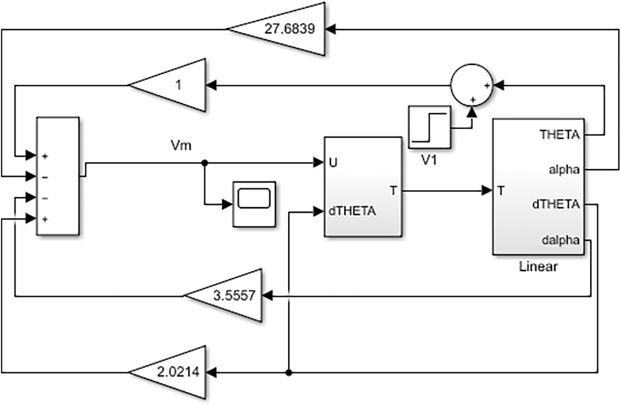
Figure 2: Simulation of the linear model with the controller in Simulink

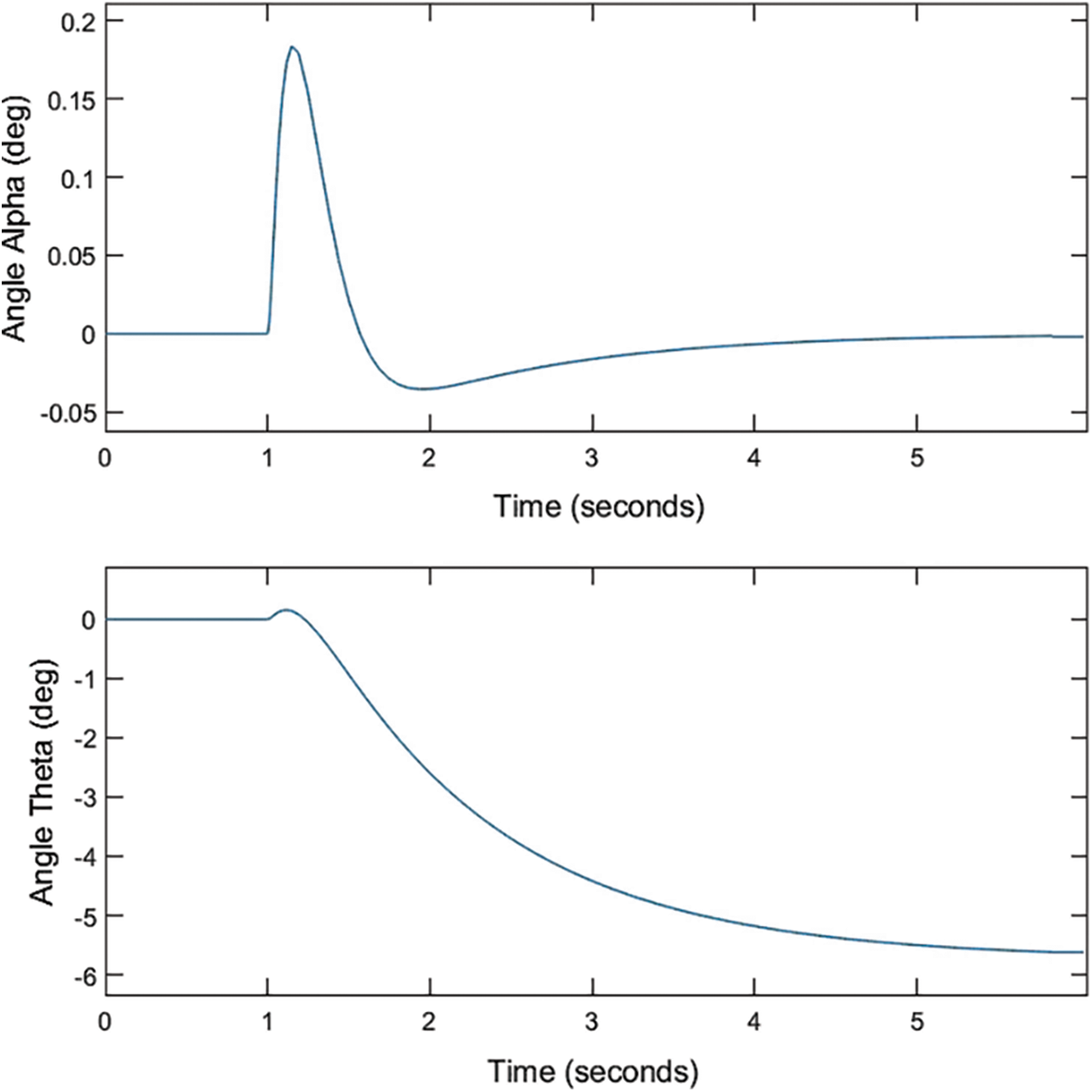
Figure 3: Simulation results of the stability analysis obtained using the MATLAB Simulink Model

4  Hardware Implementation and Validation

Hardware has been set up as shown in Fig. 4. It depicts the Rotary inverted pendulum module coupled to the Quanser SRV02 plant in the correct configuration. Quanser SRV02 has a direct current (DC) motor enclosed in an aluminum frame and is equipped with a planetary gearbox. The module is attached to the SRV02 load gear and the pendulum arm is attached to the module body. In order to keep the pendulum stable and upright, the LQR has been designed and implemented. LQR is an excellent approach that provides optimal feedback gains to make a closed-loop system robust and stable. It also provides a local approximation to develop optimal control for nonlinear systems [38].

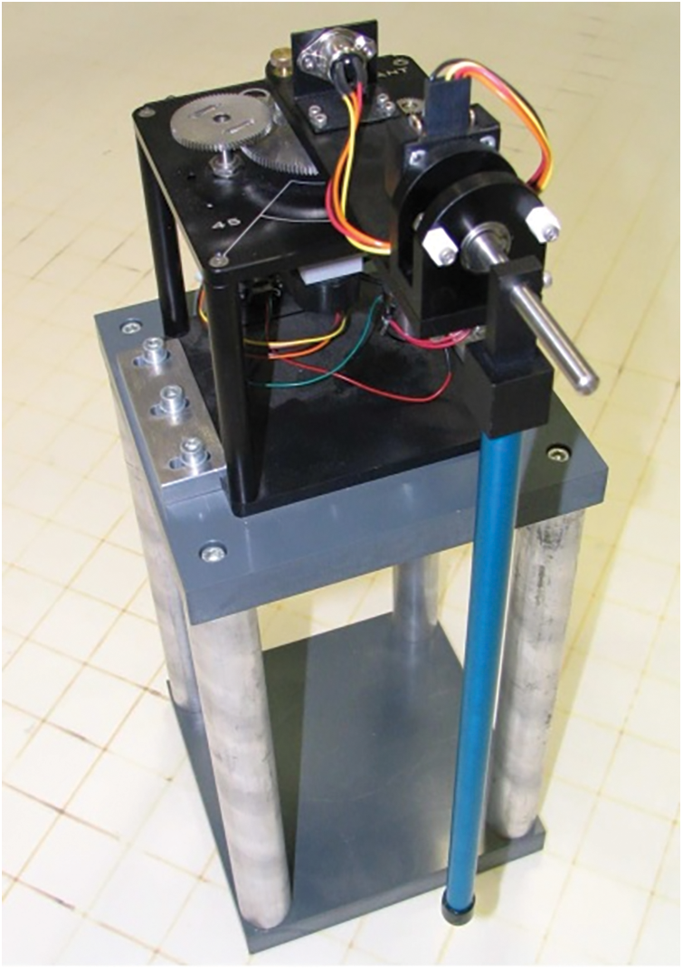
Figure 4: Hardware implementation of the rotary inverted pendulum

The designed controller has been implemented over the real inverted pendulum. The plots of variation in angles both in simulation and the real environment with the passage of time have been shown in Figs. 5 and 6. The angle in degrees is along the vertical axis versus time in seconds is along the horizontal axis as shown in Figs. 5 and 6. Fig. 6 shows the variation in the horizontal link’s angle θ and Fig. 5, shows the corresponding adjustment in the vertical arms’ angle α. The Blue dotted line represents the plot of the measured value and the green line represents the simulation results. It is clear from both plots that the actual measured values obtained from the inverted pendulum are very close to the simulated values. The presentation of the results validates the proposed controller. The horizontal link has been rotated in both directions during the simulation and real experimentation as shown in Fig. 5. The controller has adjusted the vertical angle and rejected the disturbances and kept the pendulum in a stable upright position as shown in Fig. 6. The pendulum vertical arm is swinging with a very small range showing stable behavior.

Figure 5: Variation in vertical angle alpha (simulation and measured results)

Figure 6: Variation in horizontal angle theta (simulation and measured results)

5  Conclusion and Future Work

In current research work, a state-feedback controller for the rotary inverted pendulum utilizing the LQR techniques has been designed. Mathematical modeling, linearization, simulation and validation of the designed controller over real hardware has been carried out. It is evident from the simulation and measured results that the designed controller is performing well and is robust enough to keep the pendulum in an upright stable position. For future work, a non-model-based controller or a nonlinear controller can be designed and evaluated and performance comparison can be made.

Acknowledgement: Authors would like to thank Christopher Hille for the thorough discussion.

Funding Statement: The authors received no specific funding for this study.

Conflicts of Interest: The authors declare that they have no conflicts of interest to report regarding the present study.

This work is licensed under a Creative Commons Attribution 4.0 International License, which permits unrestricted use, distribution, and reproduction in any medium, provided the original work is properly cited.