Computers, Materials & Continua DOI:10.32604/cmc.2022.028855
Article

Optimal Deep Transfer Learning Model for Histopathological Breast Cancer Classification

Mahmoud Ragab1,2,3,* and Alaa F. Nahhas4

1Information Technology Department, Faculty of Computing and Information Technology, King Abdulaziz University, Jeddah 21589, Saudi Arabia
2Center for Artificial Intelligence in Precision Medicines, King Abdulaziz University, Jeddah, 21589, Saudi Arabia
3Mathematics Department, Faculty of Science, Al-Azhar University, Naser City, 11884, Cairo, Egypt
4Biochemistry Department, Faculty of Science, King Abdulaziz University, Jeddah, 21589, Saudi Arabia
*Corresponding Author: Mahmoud Ragab. Email: mragab@kau.edu.sa
Received: 19 February 2022; Accepted: 02 April 2022

Abstract: Earlier recognition of breast cancer is crucial to decrease the severity and optimize the survival rate. One of the commonly utilized imaging modalities for breast cancer is histopathological images. Since manual inspection of histopathological images is a challenging task, automated tools using deep learning (DL) and artificial intelligence (AI) approaches need to be designed. The latest advances of DL models help in accomplishing maximum image classification performance in several application areas. In this view, this study develops a Deep Transfer Learning with Rider Optimization Algorithm for Histopathological Classification of Breast Cancer (DTLRO-HCBC) technique. The proposed DTLRO-HCBC technique aims to categorize the existence of breast cancer using histopathological images. To accomplish this, the DTLRO-HCBC technique undergoes pre-processing and data augmentation to increase quantitative analysis. Then, optimal SqueezeNet model is employed for feature extractor and the hyperparameter tuning process is carried out using the Adadelta optimizer. Finally, rider optimization with deep feed forward neural network (RO-DFFNN) technique was utilized employed for breast cancer classification. The RO algorithm is applied for optimally adjusting the weight and bias values of the DFFNN technique. For demonstrating the greater performance of the DTLRO-HCBC approach, a sequence of simulations were carried out and the outcomes reported its promising performance over the current state of art approaches.

Keywords: Breast cancer; histopathological images; machine learning; biomedical analysis; deep learning; computer vision

1  Introduction

Cancer is a crucial healthcare problem around the world. Amongst the cancer kind, breast cancer occurrence rate is the 2nd maximum for women, apart from lung cancer. Additionally, the death rate of breast tumors is advanced than other kinds of tumors [1]. Even with the fast development in medication, the study of histopathological image (HI) remains the most commonly utilized technique for breast cancer diagnoses. In each HI analysis task, the predominant is the classifier process. Since the automated and accurate classifier of higher-resolution HI is the bottleneck and cornerstone of other researches, like gland segmentation, nuclei localization, and mitosis detection [2]. At present, histopathological imaging in medical settings is mostly depending on the manual qualitative analysis of pathologists. But a minimum three problem arises from this analysis technique [3]. Firstly, there is a deficiency of pathologists, particularly in small hospitals and lesser developed areas. This unbalanced distribution and resource shortage is a crucial issue to be resolved. Next, whether the histopathological diagnoses are accurate or incorrect depends fully on the long-term accumulated diagnostic experience and pathologist philosophical professional knowledge [4]. This pathologist subjectiveness has resulted in propagation of diagnosis inconsistency. Then, the complication of the HI makes pathologists prone to inattention and fatigue. Facing this problem, it is crucial to design precise and automatic HI analytical methods, particularly classification method, to mitigate this problem [5].

But the study of HI is a time-consuming and difficult process that needs professional knowledge. Moreover, the result might be affected by the experience level of the pathologist included [6]. Thus, computer-aided analysis of HI plays a considerable part in the diagnoses of breast cancer and its prognoses. But, the procedure of designing tool for carrying out this study is obstructed by the succeeding problem. Firstly, HI of breast cancer is fine-grained, higher-resolution image that depicts complex texture and rich geometric structure [7]. The consistency between classes and the variability with a class can create classifier very hard, particularly while handling various classes. The next problem is the limitation of feature extraction method for HI of breast cancer. Deep learning (DL) techniques has the ability to learn abstract illustrations of information, extract features and retrieve data from data automatically [8]. They could resolve the problem of conventional feature extraction and be effectively employed in biomedical science, computer vision, etc.

Wei et al. [9] estimate the efficiency of Auxiliary Classifier Generative Adversarial Network (ACGAN) augmentation approach by implementing breast cancer HI classifier trained on improved dataset. For this classification, we utilize a transfer learning (TL) method wherein the convolution feature is extracted from a pertained system and next given into extreme gradient boosting (XGBoost) classifier. Gheshlaghi et al. [10] presented a hybrid convolution and recurrent deep neural network (DNN) for breast cancer HI classification. According to the rich multi-level feature illustration of the HI, the technique incorporates the advantage of convolution neural network (CNN), recurrent neural network (RNN), and long short term memory (LSTM) spatial relations among patches are conserved. Yan et al. [11] propose an attention high-order deep network (AHoNet) by instantaneously embedding attention model and higher-order statistical illustration as to residual convolution system. Firstly, AHoNet uses an effective network attention model using local cross-channel communication and non-dimension reduction to accomplish local salient deep features of breast cancer HI. Zou et al. [12], proposed a HI classification technique based on cross-domain transfer learning and multistage feature fusion (Cd-dtffNet). Firstly, a system using RL is developed that could extract features from various stages. Next, the capability to extract global features are learned by traveling from the bridge field to the target field, and the capability to extract local features are learned through travelling from the source field to bridge field.

Wang et al. [13] introduce a breast tumor HI classification by assembling compact CNN. Firstly, a hybrid CNN method is developed that comprises global and local model branch. With local voting and two-branch data integration, the hybrid method attains strong representative capability. Next, by embedded the presented Squeeze-Excitation-Pruning (SEP) as to hybrid method, the network significance is learned and the unwanted channel is eliminated. Zhu et al. [14] propose a CNN that involves a convolution layer, smaller (SE)-ResNet model, and fully connected layer. Then, presented a smaller SE-ResNet model that is a development on the integration of residual model and SE block, and accomplishes the similar efficiency with less parameter. Additionally, presented a learning rate scheduler that could attain outstanding results without finetuning the learning rate.

This study develops a Deep Transfer Learning with Rider Optimization Algorithm for Histopathological Classification of Breast Cancer (DTLRO-HCBC) technique. The proposed DTLRO-HCBC technique undergoes pre-processing and data augmentation to increase quantitative analysis. In addition, optimal SqueezeNet model is employed for feature extractor and the hyperparameter tuning process is carried out using the Adadelta optimizer. Besides, rider optimization with deep feed forward neural network (RO-DFFNN) technique was utilized for breast cancer classification (BCC). For demonstrating the greater performance of the DTLRO-HCBC system, a sequence of simulations was carried out.

2  The Proposed Model

This study has developed a new DTLRO-HCBC system for BCC and detection. The proposed DTLRO-HCBC technique aims to categorize the existence of breast cancer using histopathological images. The DTLRO-HCBC technique comprises a sequence of processes namely pre-processing, SqueezeNet based feature extraction, Adadelta hyperparameter optimizer, DFFNN classifier, and RO parameter optimization.

2.1 Stage I: Feature Extraction

Next to image pre-processing, the optimal SQNet model is employed as feature extractor. SQNet is a convolutional system that outperformed AlexNet when utilizing 50x parameterss [15,16]. It has 18 layers, involving max-pooling (MXP), Global Average Pooling (GAP), convolutional layer, softmax output layer, and fire levels. The input has 227 × 227-dimension images and contains RGB channels. Convolution is utilized for generalizing the max pooling and input image. Since the positive module, all the convolutional layer implements element-wise activation. Amongst the convolutional layers, SQNet utilizess the fire layers that aree composed of squeeze and expansion stages. The squeezing procedure decreases the depth, while the expanding phase rises when preserving a similar feature size. At last, with the merging process, the expanding output is arranged in the dimension of the input.

Lastly, the resulting f(y) of the squeezing procedure with the feature maps (FM), kernel (W), and C specifies channel of tensor correspondingly:

 f(y)=∑fm=1FM⁡∑c=1C⁡Wcf∗xcfm (1)

whereas f(y) denotes an output ∈ RN. Assume Xi indicate input with size of (Wi, Hi, Ci) ∈ RN of layer i. W represents the weight, H determines the height, and C indicates the channel correspondingly. The MXP layer and spatial dimension execute downsampling in the system and the GAP, that convert the feature map class as to individual value. Finally, Softmax activation function produces multiclass probability distribution.

The hyperparameters involved in the SQNet model can be modified by the use of Adadelta optimizer. Adadelta [17] is an extension of Adagrad to observe reducing learning rate. The running average E[g2]t at time step t later only depending on the preceding average and the existing gradient.

E[g2] =γE[g2]t−1+(1−γ)gt2(2)

Next set γ to same value as momentum, about 0.9. For clearness, rewrite vanilla stochastic gradient descent (SGD) upgrade interms of the variable upgraded vector △θt:

△θt=−α.gt,i(3)

△θt+1=θt+δθt(4)

The variable upgrade vector of Adagrad is previously acquired from the following:

△θt=−αGt+ε⊙gt (5)

While the denominator represents the root mean squared (RMS) error condition of the gradient, then substitute with the standard short-hand:

△ θt=−αRMS[g]t(6)

The author noted that the unit in this upgrade (SGD, Momentum, or Adagrad) must have a similar hypothetical unit as the variable. To understand this, firstly determine exponentially decaying average, squared gradient, and parameter upgrades.

E[△ θ2]t=γE△ θt−12+(1−γ)△ θt2(7)

The root means squared error of variable upgrades as follows:

RMS[△ θ]t=E[△ θ2]t+ε (8)

Replace the learning rate in the preceding upgrade rule with the RMS of variable upgrade. lastly produces the Adadelta upgrade rules:

△ θt=−RMS[△ θ]RMS[g]t(9)

θt+1=θt+△ θt(10)

Using Adadelta, they don't want to set default learning rate, since it was removed from the upgrade rules.

2.2 Stage II: Image Classification

At the time of BCC, the features are passed into the DFFNN model to categorize the images. Assume the DFFNN encompasses of single input layer, m hidden layers, and single output layer [18]. The input layer states input parameter x∈X and feeds a vector. Fig. 1 depicts the framework of DFFNN.

f(0)(x)=[h1(0)(x), …, hk0(0)(x)]T∈Rk0      (11)

to the primary hidden layer, whereas k0 denotes the amount of layer in the input neuron and hj(0):X↦R indicates the activation function of j-th layer in the input layer. For each i=1,…,m, the i-th hidden neuron declare f(i−1)(x)∈Rki−1 from the preceding layer and constructed a vector f(i)(x)∈Rki, widely named a feature, as follows

f(i)(x)=[h(i)(w1(i)Tf(i−1)(x)+b1(i)),…,h(i)(wki(i)Tf(i−1)(x)+bki(i))]T,(12)

whereas ki indicates the amount of layers in the i-th hidden state, h(i) : R↦R shows the activation function in i-th hidden state, wj(i)∈Rki−1 and bj(i)∈R indicates the weight vector and bias of j−th layer in the i−th hidden state, correspondingly. Signify W(i)=[w1(i), …, wki(i)] and b(i)=[b1(i), …, bki(i)]T, (12) is formulated by

f(i)(x)=h(i)(W(i)Tf(i−1)(x)+b(i)),(13)

whereas h(i) : Rki↦Rki shows a vector-valued function. For notational simplicity, consider k=km and f(x)=f(m)(x). The output neuron states f(x)∈Rk from the previous hidden layer and produced an output vector a(x)∈Hn, named an action, as follows

a(x)=h(WTf(x)+b)=[h(w1Tf(x)+b1), ⋯, h(wnTf(x)+bn)]T,(14)

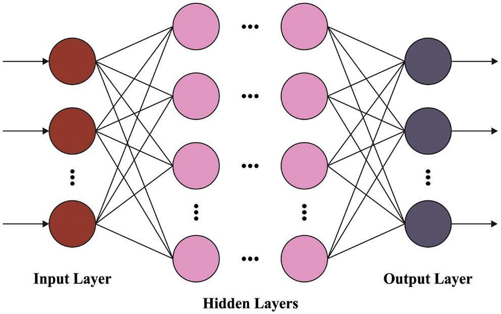
Figure 1: DFFNN structure

Her n shows the amount of neurons, h:R↦H indicates the activation function in the output layer, H indicates the image set of h with H⊆R,wj∈Rk and bj∈R denotes the weight vector and bias of the j-th layer in the output layer, correspondingly, W=[w1, …, wn] and b=[b1, …, bn]T.

2.3 Stage III: Parameter Optimization

To effectually tune the parameters presented in the DFFNN technique, the RO approach has been utilized. The inspiration for emerging ROA [19] is attained from the race occurring amongst the collection of riders to accomplish the target. Now, attacker, bypass rider, follower, and overtaker are the 4 classes that are considered in ROA. The overall amount of riders is splitted into 4 classes of riders. All the groups of riders pose the winning approach to achieve the aim. By avoiding the bypass rider neglects the primary route to accomplish the target. Now, the followers follow the route of primary rider. According to the primary rider, the overtaker proceeds in their individual location to attain the target. The maximal speed is employed by the attackers to accomplish the target position by considering the rider's location. In the following, seven steps included in ROA are mentioned in the following.

1.    Rider and group parameters Initialization: here, the follower, bypass rider, attacker, and overtaker are collectively represented as E and the position of rider is arbitrarily initialized. The group initialization can be expressed by

St={St(u, v)} 1≤u≤D 1≤v≤R(15)

Here, the overall amount of riders included in the competition is represented as D. The dimension or number of co-ordinates is denoted as R, and at time t the uth location of the rider is signified as Stuv. The amount of riders contributing to the competition is defined by the overall amount of riders existing in all the groups as follows.

D=M+L+Q+T(16)

The M,L,Q and T variables are utilized for representing the overall amount of bypass rider, follower, overtaker, and attacker.

Also, the rider variables namely gear, steering, brake, and accelerator are initialized afterward the group initialization [20]. Now, the parameter A is utilized for denoting steering direction. It can be expressed as follows

At={Au,vt}1≤u≤D 1≤v≤R(17)

Now, the steering direction of uth rider vehicles are represented as Au,vt. The steering initialization direction while the time is zero is shown below

Au,v={θjif v=1Au,v−1+ϕif v≠1&Luiv−1+ϕ≤360Au,v−1+ϕ≤360otherwise(18)

The θi and ϕ are uth rider vehicle location and coordinate angles.

2.   To describe the success rate: All the riders should be described according to the distance when the group initialization and rider parameter is completed.

wu=1||Su−HA||(19)

Here, the uth rider location is denoted as Su and the location of target is shown as HA.

3.   To determine the primary rider: while determining the primary rider, the success rate served a critical role. The primary rider isn't constant since the rider location differs at all time limits. Thus, depending on the success rate, rider becomes the primary rider.

4.   To upgrade the location of the rider: The rider position is upgraded for discovering the primary rider that is winner in all the sets.

Upgrade location of bypass rider: while the bypass rider neglects the conventional route utilized by another rider, the location Upgrade can be performed in an arbitrary way for the bypass rider as in the following

St+1M(u, v)=δ[St(η, v)⋆β(v)+St(ξ,v)⋆[1−β(v)]](20)

Here, the arbitrary number of δ ranging from 0 to 1, the arbitrary number of η ranging from 1 to D, the arbitrary number of ξ ranging from 1 to D and the arbitrary number of β ranging from 0 to 1.

ii) Upgrade the location of follower: The arithmetical equation to upgrade the place of the follower is as follows

S+1L(u,p)=SH(H,p)+[cos(Au,pt)⋆SH(H,p)⋆but](21)

Now, the coordinate selector is represented as p,SH denotes the location of the primary rider, H indicates the index of primary rider, and but shows the distance covered by the uth rider.

iii) Upgrade the location of over taker: here, three significant factors should be taken into account namely the success rate, the direction indicator, and the coordinate selector.

St+1Q(u,p)=St(u,p)+[Ytj(u)∗SH(H,p)] (22)

iv) Upgrade the location of the attacker: Although the attacker goals to accomplish the location of the leader, the location Upgrade equation of the follower is utilized for upgrading the location of the attacker.

St+1T(u, v)=SH(H, v)+[cos(Au,vt)⋆SH(H, v)]+but(23)

Now SH(H,v) signifies the location of the primary rider and the steering direction of the uth rider of the vth coordinate is denoted as Au,vt.

5.   Describe the success rate again: Finally, rider finished the location upgrade method, the success rate can be evaluated by the rider's new location, and the existing primary rider could be recognized.

6.   Upgrade the Rider constraint: It is important to upgrade the variable of the rider to obtain the optimum solution. Additionally, constraints such as activity, counter is also upgraded that facilitate upgrading the gear values and steering angle.

7.   End procedure: The above-mentioned steps should be continuously iterated until the end time (Toff) and within that time, the primary rider should be identified that is taken into account as the winner of the bike competition. Fig. 2 illustrates the steps involved in ROA technique.

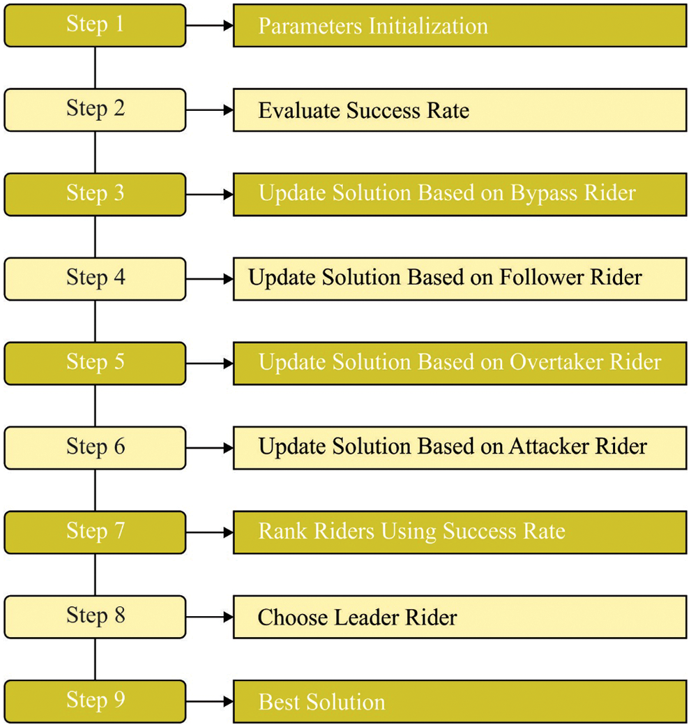
Figure 2: Steps involved in RO technique

3  Experimental Validation

In this section, the DLTRO-HCBC technique is simulated using a set of HIs collected from various sources. The experimental results of the DLTRO-HCBC technique are investigated under distinct sizes of training/testing data. A few sample images are demonstrated in Fig. 3.

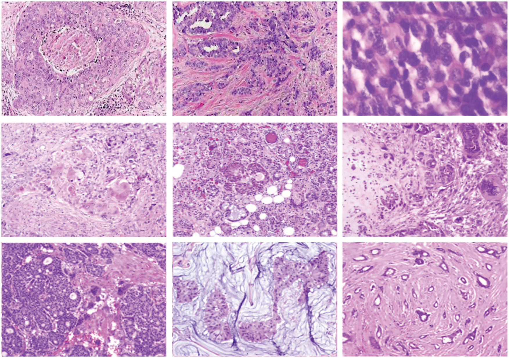
Figure 3: Sample images

Tab. 1 provides detailed breast cancer classifier results of the DLTRO-HCBC technique. Fig. 4 establishes the classification outcomes of the DLTRO-HCBC technique on testing or training data of 80:20. The figure illustrated that the DLTRO-HCBC technique has proficiently identified all three classes. For sample, the DLTRO-HCBC system has identified Normal class with precn of 94.02%, recal of 94.12%, accuy of 92.16%, Fscore of 92.88%, and Mathew Correlation Coefficient (MCC) of 93.40%. Meanwhile, the DLTRO-HCBC technique has identified Benign class with precn of 94.07%, recal of 92.14%, accuy of 92.55%, Fscore of 93.93%, and MCC of 93.74%. Eventually, the DLTRO-HCBC technique has identified Invasive Carcinoma class with precn of 92.41%, recal of 94.17%, accuy of 94.08%, Fscore of 94.11%, and MCC of 92.14%. Fig. 5 proves the classification results of the DLTRO-HCBC method on training/testing data of 70:30. The figure illustrated that the DLTRO-HCBC technique has proficiently identified all three classes. For example, the DLTRO-HCBC system has identified Normal class with precn of 92.42%, recal of 94.17%, accuy of 93%, Fscore of 93.48%, and MCC of 92.37%. Meanwhile, the DLTRO-HCBC technique has identified Benign class with precn of 92.05%, recal of 92.46%, accuy of 91.46%, Fscore of 94.26%, and MCC of 93.34%. At last, the DLTRO-HCBC technique has identified Invasive Carcinoma class with precn of 93.54%, recal of 94.03%, accuy of 93.91%, Fscore of 91.87%, and MCC of 93.35%.

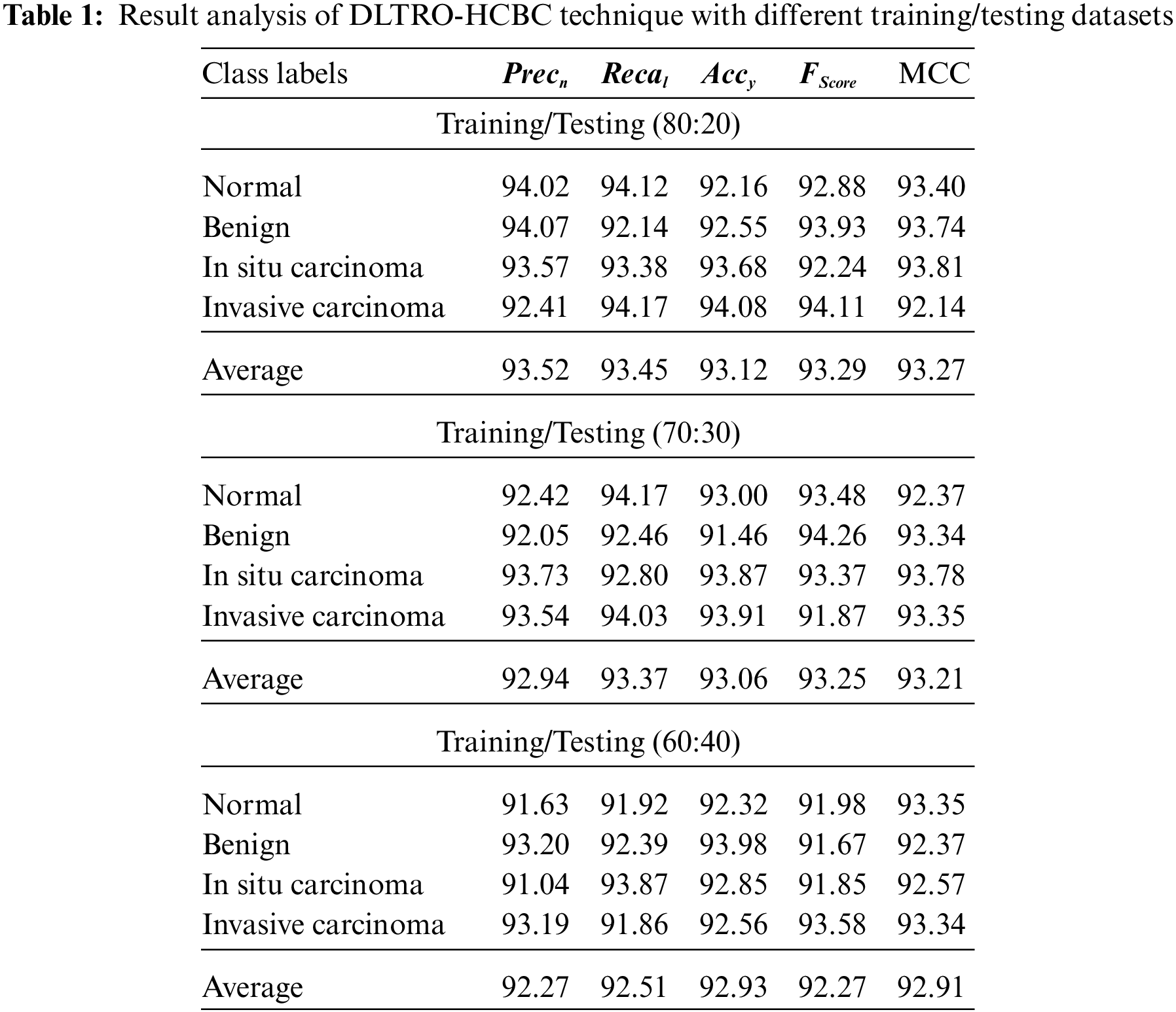
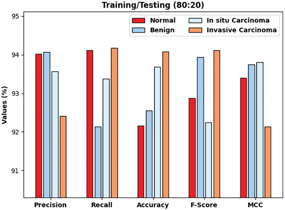
Figure 4: Result analysis of DLTRO-HCBC technique under training/testing of 80:20 dataset

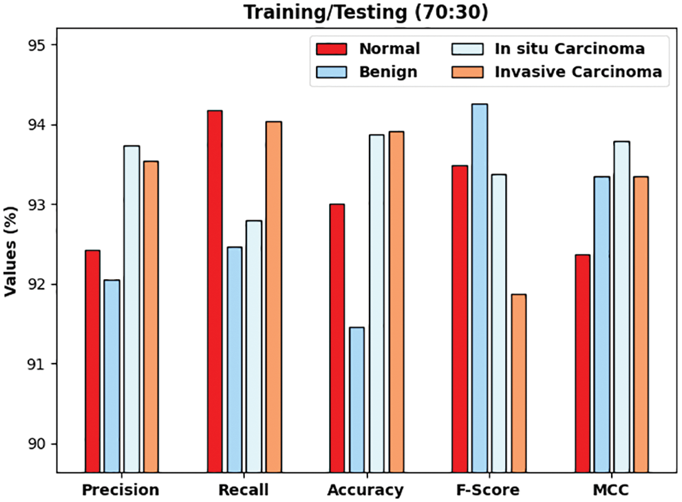
Figure 5: Result analysis of DLTRO-HCBC technique under training/testing of 70:30 dataset

Fig. 6 determines the classification results of the DLTRO-HCBC technique on training/testing data of 60:40. The figure illustrated that the DLTRO-HCBC technique has proficiently identified all three classes. For example, the DLTRO-HCBC system has identified Normal class with precn of 91.63%, recal of 91.92%, accuy of 92.32%, Fscore of 91.98%, and MCC of 93.35%. Meanwhile, the DLTRO-HCBC technique has identified Benign class with precn of 93.20%, recal of 92.39%, accuy of 93.98%, Fscore of 91.67%, and MCC of 92.37%. Finally, the DLTRO-HCBC technique has identified Invasive Carcinoma class with precn of 93.19%, recal of 91.86%, accuy of 92.56%, Fscore of 93.58%, and MCC of 93.34%.

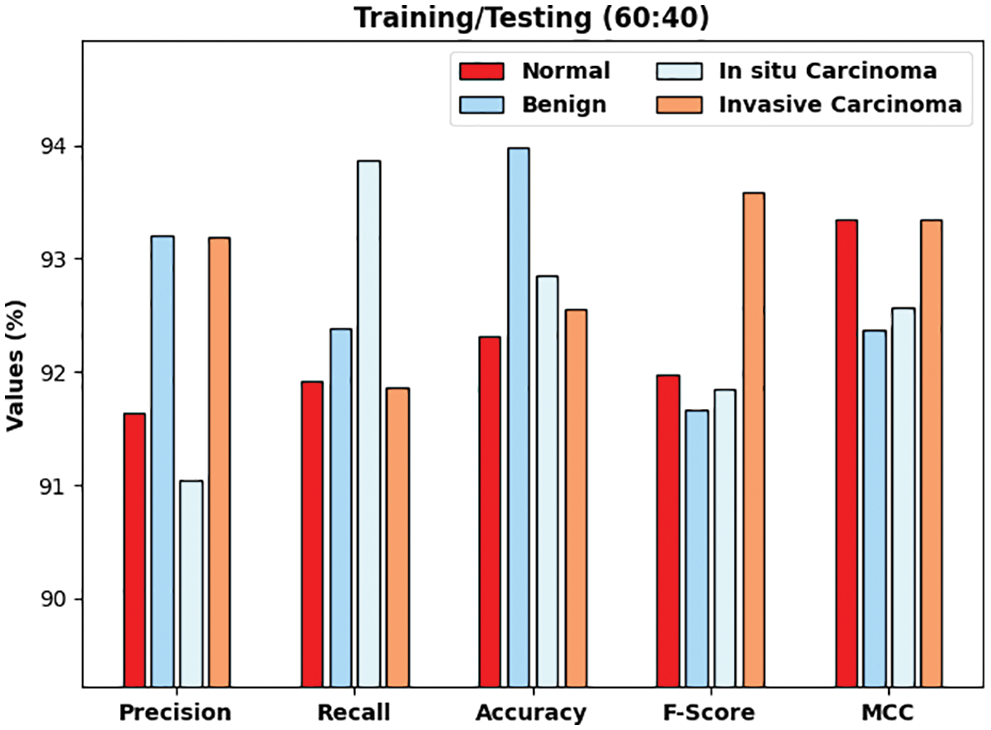
Figure 6: Result analysis of DLTRO-HCBC technique under training/testing of 60:40 dataset

Fig. 7 illustrates the experimental validation of the DLTRO-HCBC technique on training/testing data of 80:20. The figure portrayed that the DLTRO-HCBC technique has obtained precision of 93.52% and recall of 93.45%. At the same time, the DLTRO-HCBC technique has resulted in accuracy of 93.12% and F-score of 93.29%. Besides, the DLTRO-HCBC technique has obtained MCC of 93.27%.

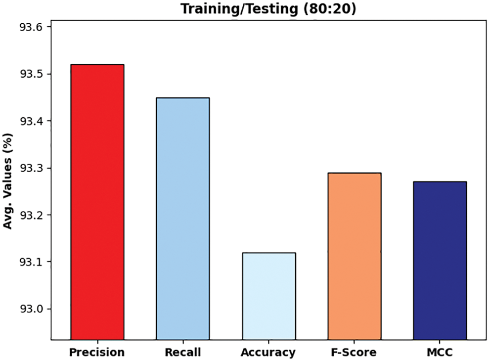
Figure 7: Overall analysis of DLTRO-HCBC technique under training/testing of 80:20 dataset

Fig. 8 validates the accuracy assessment of the DLTRO-HCBC model under training and testing of 80:20 dataset. The results described that the DLTRO-HCBC model has the aptitude of gaining improved values of training and validation accuracies. It is visible that the validation accuracy values are slightly higher than training accuracy.

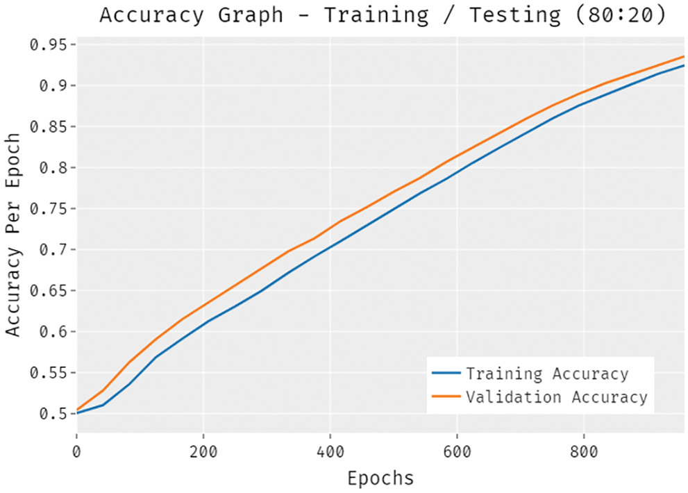
Figure 8: Accuracy analysis of DLTRO-HCBC technique under training/testing of 80:20 dataset

A brief training and validation loss offered by the DLTRO-HCBC model are reported in Fig. 9 under training and testing of 80:20 dataset. The results revealed that the DLTRO-HCBC model has accomplished minimum values of training and validation losses.

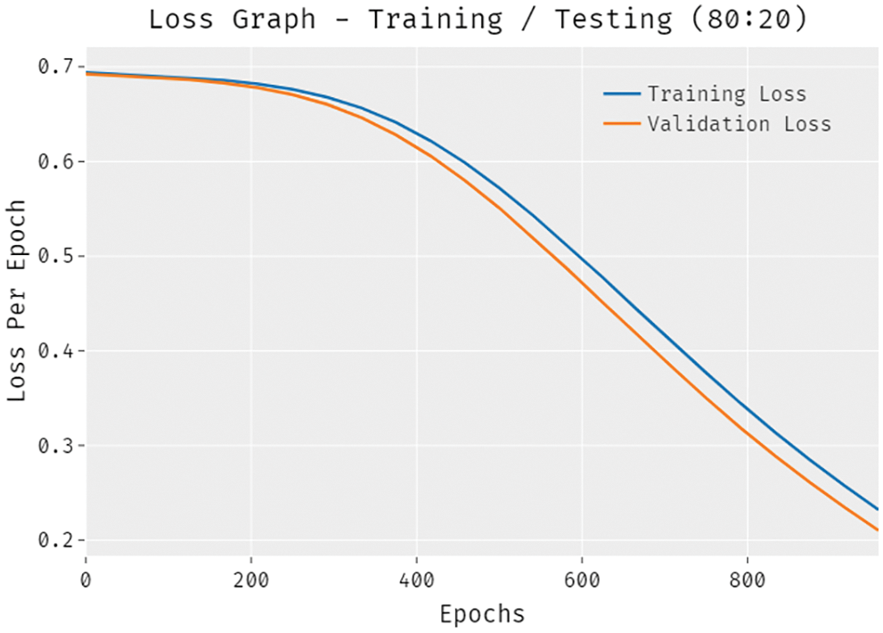
Figure 9: Loss analysis of DLTRO-HCBC technique under training/testing of 80:20 dataset

Fig. 10 illustrates the experimental validation of the DLTRO-HCBC technique on training/testing data of 70:30. The figure portrayed that the DLTRO-HCBC technique has obtained precision of 92.94% and recall of 93.37%. At the same time, the DLTRO-HCBC technique has resulted in accuracy of 93.06% and F-score of 93.25%. Besides, the DLTRO-HCBC technique has obtained MCC of 93.21%.

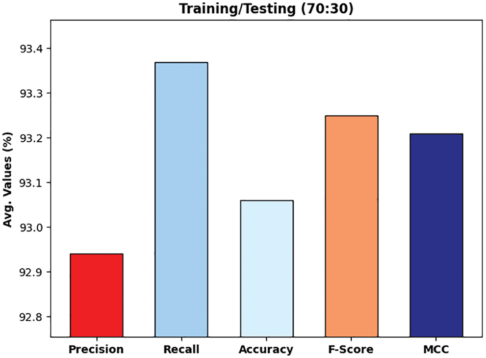
Figure 10: Overall analysis of DLTRO-HCBC technique under training/testing of 70:30 dataset

Fig. 11 validates the accuracy assessment of the DLTRO-HCBC model under training and testing of 70:30 dataset. The results described that the DLTRO-HCBC model has the aptitude of gaining improved values of training and validation accuracies. It is visible that the validation accuracy values are slightly higher than training accuracy.

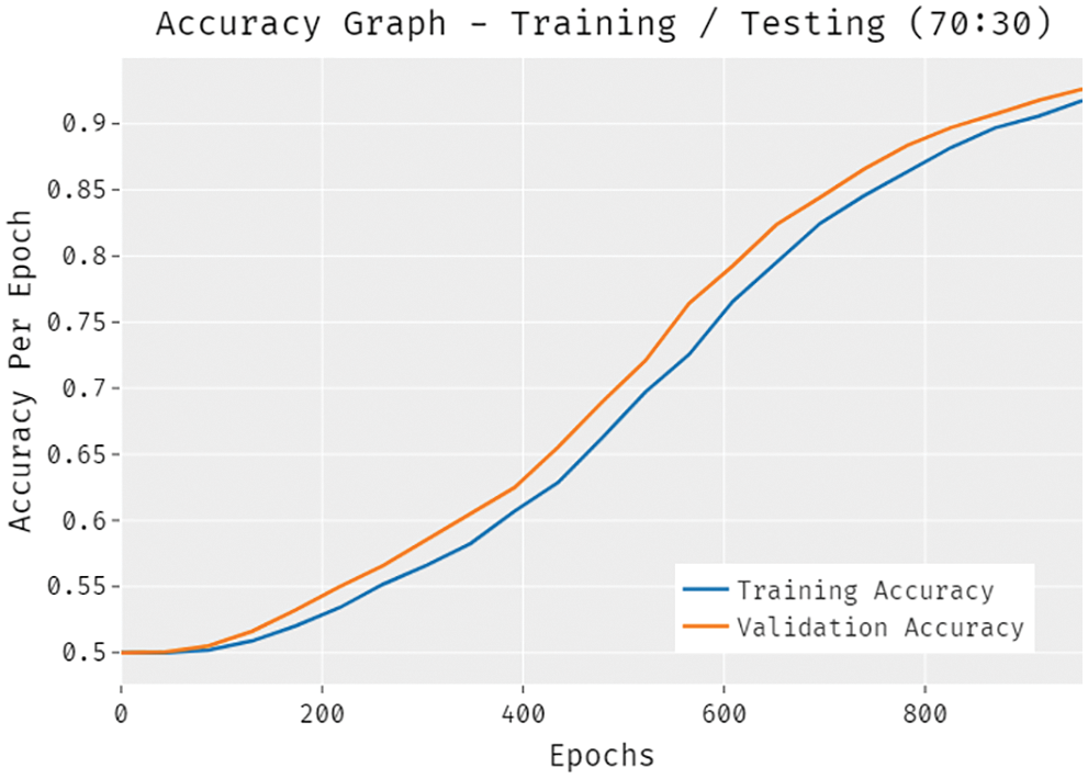
Figure 11: Accuracy analysis of DLTRO-HCBC technique under training/testing of 70:30 dataset

A brief training and validation loss offered by the DLTRO-HCBC model are reported in Fig. 12 under training and testing of 70:30 dataset. The outcomes revealed that the DLTRO-HCBC model has gained minimum values of training and validation losses.

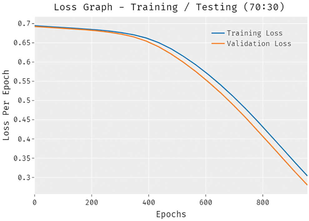
Figure 12: Loss analysis of DLTRO-HCBC technique under training/testing of 70:30 dataset

Fig. 13 illustrates the experimental validation of the DLTRO-HCBC technique on training/testing data of 60:40. The figure portrayed that the DLTRO-HCBC technique has obtained precision of 92.27% and recall of 92.51%. At the same time, the DLTRO-HCBC technique has resulted in accuracy of 92.93% and F-score of 92.27%. Besides, the DLTRO-HCBC technique has obtained MCC of 92.91%.

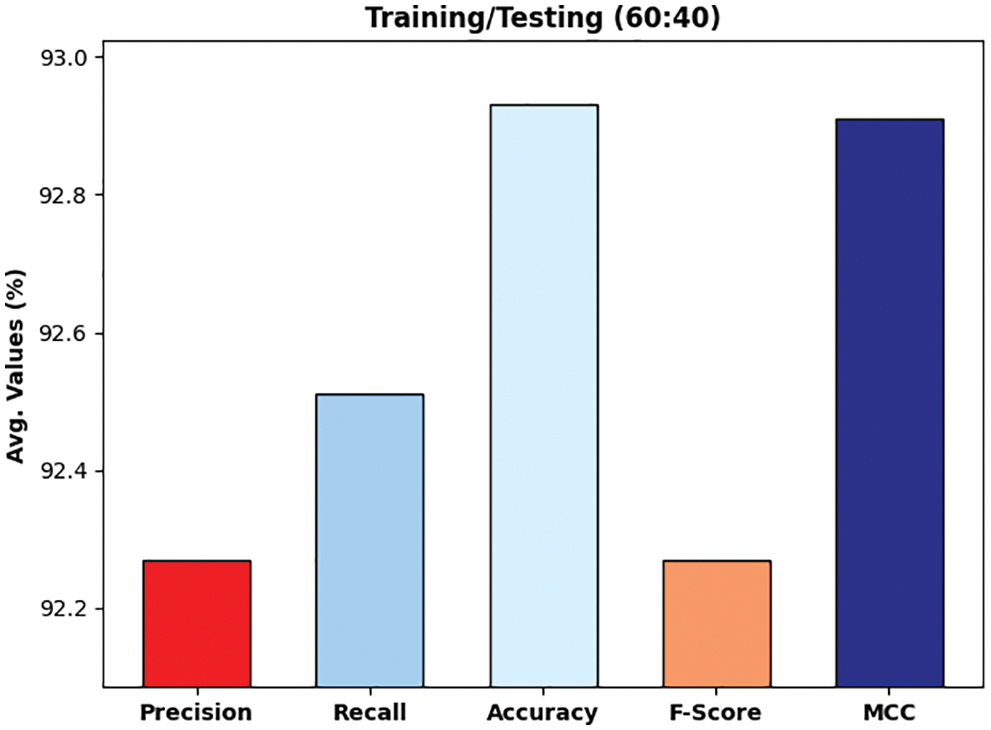
Figure 13: Overall analysis of DLTRO-HCBC technique under training/testing of 60:40 dataset

Tab. 2 and Fig. 14 highlights the comparative accuracy analysis of the DLTRO-HCBC technique. The results indicated that the VGG16 system has demonstrated poor results with least accuracy of 80.35%. Simultaneously, the ResNet-50 and Inception v3 techniques have resulted in somewhat enhanced accuracy of 82.54% and 81.97% correspondingly. Also, the Incep. V3-LSTM model has accomplished reasonable results with an accuracy of 91.24%. Though the Incep. V3-bidirectional LSTM (BiLSTM model has resulted in competitive outcome with an accuracy of 92.45%, the DLTRO-HCBC technique has reached maximum accuracy of 93.12%. After examining the above-mentioned tables and figures, it can be clear that the DLTRO-HCBC method has gained maximum outcome on BCC.

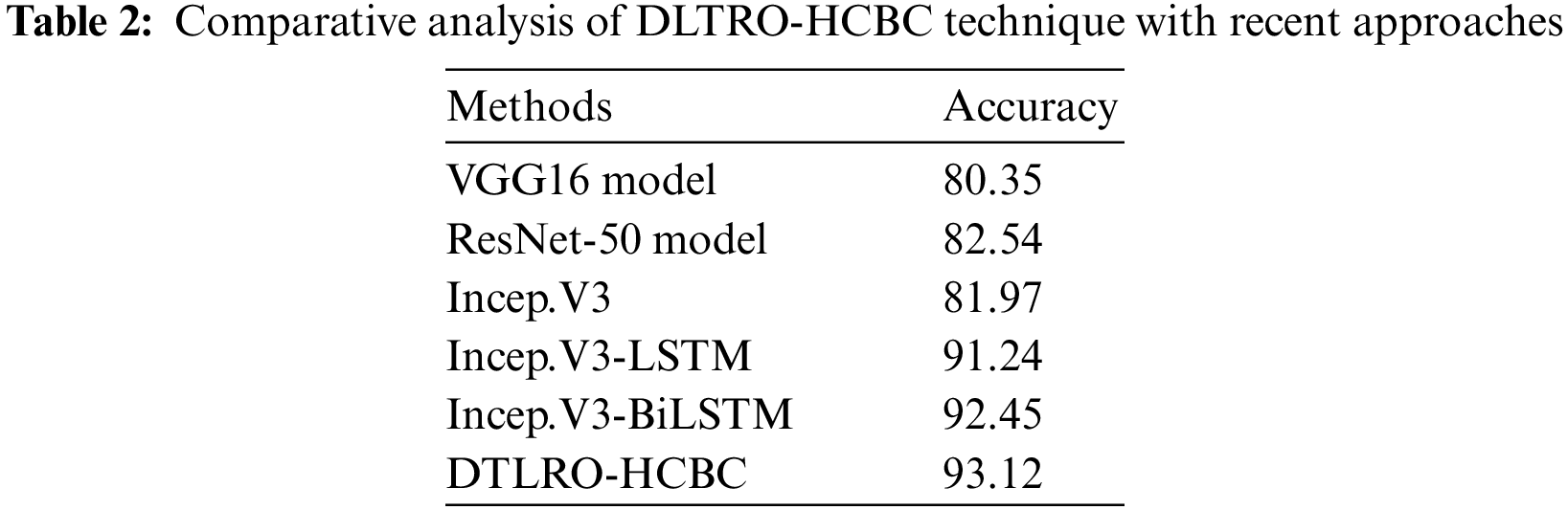
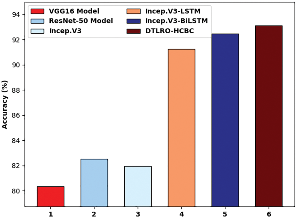
Figure 14: Comparative analysis of DLTRO-HCBC technique with recent approaches

4  Conclusion

The latest advances of DL models help in accomplishing maximum image classification performance in several application areas. This study has developed a new DTLRO-HCBC system for breast cancer detection and classification. The proposed DTLRO-HCBC technique aims to categorize the existence of breast cancer using histopathological images. The DTLRO-HCBC technique comprises a series of processes i.e., pre-processing, SqueezeNet based feature extraction, Adadelta hyperparameter optimizer, DFFNN classifier, and RO parameter optimization. The RO algorithm is applied for optimally adjusting the weight and bias values of the DFFNN model. The experimental results of the DLTRO-HCBC technique are investigated under distinct sizes of training/testing data. For demonstrating the greater performance of DTLRO-HCBC process, a sequence of simulations was carried out and the outcomes reported its promising performance over the recent approaches. In future, hybrid metaheuristics can be employed for hyperparameter tuning process.

Acknowledgement: This work was funded by the Deanship of Scientific Research (DSR), King Abdulaziz University, Jeddah, under grant no. (D-773-130-1443). The authors, therefore, gratefully acknowledge DSR technical and financial support.

Funding Statement: This project was funded by the Deanship of Scientific Research (DSR), King Abdulaziz University, Jeddah, under grant no. (D-773-130-1443).

Conflicts of Interest: The authors declare that they have no conflicts of interest to report regarding the present study.

This work is licensed under a Creative Commons Attribution 4.0 International License, which permits unrestricted use, distribution, and reproduction in any medium, provided the original work is properly cited.