Computers, Materials & Continua DOI:10.32604/cmc.2022.029542
Article

Multi-Level Feature Aggregation-Based Joint Keypoint Detection and Description

Jun Li1, Xiang Li1, Yifei Wei1,*, Mei Song1 and Xiaojun Wang2

1Beijing Key Laboratory of Work Safety Intelligent Monitoring, School of Electronic Engineering, Beijing University of Posts and Telecommunications, Beijing, 100876, China
2Dublin City University, Dublin, 9, Ireland
*Corresponding Author: Yifei Wei. Email: weiyifei@bupt.edu.cn
Received: 06 March 2022; Accepted: 26 April 2022

Abstract: Image keypoint detection and description is a popular method to find pixel-level connections between images, which is a basic and critical step in many computer vision tasks. The existing methods are far from optimal in terms of keypoint positioning accuracy and generation of robust and discriminative descriptors. This paper proposes a new end-to-end self-supervised training deep learning network. The network uses a backbone feature encoder to extract multi-level feature maps, then performs joint image keypoint detection and description in a forward pass. On the one hand, in order to enhance the localization accuracy of keypoints and restore the local shape structure, the detector detects keypoints on feature maps of the same resolution as the original image. On the other hand, in order to enhance the ability to percept local shape details, the network utilizes multi-level features to generate robust feature descriptors with rich local shape information. A detailed comparison with traditional feature-based methods Scale Invariant Feature Transform (SIFT), Speeded Up Robust Features (SURF) and deep learning methods on HPatches proves the effectiveness and robustness of the method proposed in this paper.

Keywords: Multi-scale information; keypoint detection and description; artificial intelligence

1  Introduction

Finding the pixel-level connection between images is a basic step in many computer vision tasks such as Simultaneous Localization and Mapping (SLAM) [1], Structure from Motion (SfM) [2] and image matching [3,4]. Image keypoint detection and description is a popular method to achieve this connection [5–7]. As these tasks are faced with increasingly challenging scenes, such as indoor/outdoor scenes, illumination and weather changes. Thus, the positioning accuracy of keypoint and generation of robust and discriminative descriptors are very important.

In the past decades, many excellent algorithms have been proposed to complete joint local keypoint detection and description [8], such as SIFT [9], ORB [4], SURF [10] and other manually designed feature algorithms. With the rapid development of deep learning [11–14], more and more image matching methods based on deep learning have been proposed, such as D2-Net [15], SuperPoint [16] and ASLFeat [17]. However, few methods are robust in complex scenarios. What’s more, most of the existing method based on deep learning tend to use the deepest features, which are shrunk several times (usually 4 or 8 times) compared to the original image for keypoint detection and description. This is yet to be optimized, because locating the coordinates of the keypoints in the deep feature maps will inevitably reduce the detection accuracy of the keypoints. At the same time, in the deep feature maps, the keypoints of different local structures may share the same high-level semantic information, which makes it difficult to extract distinguishing keypoint descriptors that retain rich local structural information.

The contributions of this paper are as follows: in order to solve the above problems, a new self-supervised deep learning method is proposed. This paper proposes two lightweight but effective modules: the keypoint detector and the keypoint descriptor. As the backbone feature encoder shares most of the calculations of these two modules, the network improves the positioning accuracy of keypoints and the discrimination of descriptors with a small computation cost. A detailed comparison with traditional feature-based methods SIFT, SURF and deep learning methods on HPatches [18] proves the effectiveness and robustness of the method proposed in this paper. The keypoint detector reorganizes the multi-level low-resolution feature maps into the original resolution of input images by bilinear up-sampling. So, keypoints are detected on the feature maps of the original image size, thus the positioning accuracy of the keypoints is improved. The keypoint descriptor aggregates multiple layers of features together to generate descriptors with rich local structure information. The example results of visual keypoints matching of the proposed network are shown in Fig. 1.

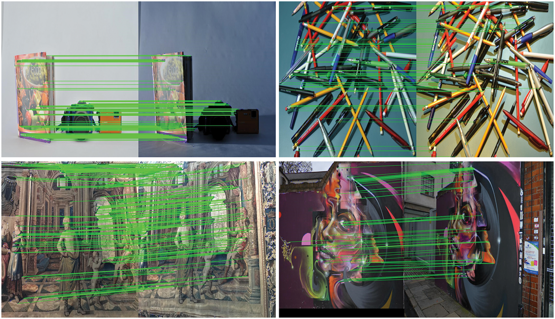
Figure 1: Visualization samples of matching keypoints on HPatches [18]. The proposed method can successfully find image correspondences even under big illumination or view point changes

2  Related Research

Joint local feature detection and description has been studied for a long time. SIFT, Oriented Fast and Rotated Brief (ORB), SURF and other hand-designed feature algorithms have achieved good results. Among these methods, SIFT occupies the mainstream position. SURF is the fast version of SIFT, while ORB is more efficient than these two algorithms and is suitable for tasks requiring high real-time requirements.

With the rise of deep learning, more and more methods have been proposed. Early methods follow the strategy of traditional feature extraction algorithms to detect firstly and then describe, and improve performance by replacing a certain step of keypoint detection or description with a learning method. For example, L2-Net [19] uses a hand-designed algorithm to detect keypoints and a convolutional neural network to generate descriptors. After that, Lf-Net [20] uses two sub-neural networks for keypoint detection and description respectively. Recently, the joint learning of detectors and descriptors has attracted more and more attention. The latest methods usually build a unified feature extraction network to extract deep features, then combining the two parts up, so as to achieve the result of sharing most of the calculation amount of the two tasks and real-time keypoints detection and description. D2-Net [15] uses dense feature description to detect keypoints at first, then closely combines detection loss and description loss to obtain a more integrated architecture. On the basis of D2-Net, ASLFeat [17] utilizes peak detection to detect keypoint on multi-level feature maps, greatly improving the positioning accuracy of keypoints. Since it is very difficult to obtain the ground truth labels for keypoint detection, SuperPoint [16] uses Homographic Adaptation to generate the keypoint labels, then trains the keypoint detector and descriptor together in a self-supervised way. However, most methods detect and describe keypoints on the deepest feature maps that are several times smaller than the original images, which needs to be optimized. In order to improve the network's perception ability and positioning accuracy of local shapes, two effective modules are proposed in this paper. The feature detector reorganizes the low-resolution feature maps of multiple layers to the original image resolution in a non-learning way, so as to improve the accuracy of keypoint location. The descriptor aggregates the multi-layer features together to generate descriptors with rich local structure information.

3  Proposed Method

3.1 Problem Statement

Geometric registration (or alignment) is a critical task in computer vision. The purpose of image registration is to find the optimal rigid perspective transformation matrix H to put the two images into the same coordinate. Assuming two images source image Ip and target image Iq, the coordinate transformation relationship between them is:

Ip=warp (Hpq,Iq)(1)

Image keypoint detection and description is a key step for finding this connection. However, due to the changes in the environment when the images are captured and the large baseline case, it is not easy to find keypoints stably and accurately, and to generate robust keypoint descriptors.

3.2 Network Architecture

The model proposed in this paper takes an image as input and outputs the keypoint map and corresponding descriptors. As shown in Fig. 2.

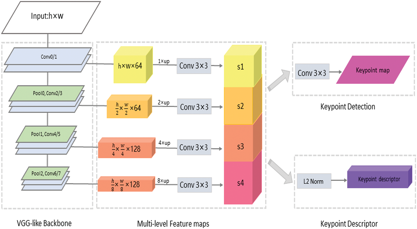
Figure 2: Proposed network architecture, including VGG-like backbone feature encoder, keypoint detection module and keypoint description module. The layers of different colors in the backbone network represent the pooling layers and the convolutional layers, the spatial down-sampling is performed through three pooling layers. The proposed network takes a single image as input, and obtains multi-scale feature maps in a forward pass. These feature maps are restored to the original image resolution by bilinear up-sampling, and then the aliasing effect from up-sampling is reduced by 3 × 3 convolution layers on each level [21]. The obtained features on different levels are aggregated by channel-wise concatenation. Then the network performs keypoint detection and description jointly

This model consists of three parts: VGG-like backbone feature encoder, keypoint detection module and keypoint description module. The proposed network up-samples the deep feature maps to the resolution of the input image, then combines the four layers of feature maps in the feature channel and feeds them into the keypoint detection and description module, thus sharing most of the computation of these two modules for efficient joint feature detection and description.

3.2.1 Backbone Feature Encoder

The VGG-like backbone feature encoder operates on full-size images. It contains 8 convolutional layers and 3 pooling layers, which executes three times space down-sampling. The steps of all convolutional layers are set to 1. The proposed multi-scale feature aggregation is performed in one forward pass. The input is I∈Rh×w, so the output features of Conv1, Conv3, Conv5 and Conv7 layers are Pi∈Rhi×wi×Ci. Where C∈{64,64,128,128},i∈{1,3,5,7}, hi∈{H,H2,H4,H8} (the same for wi). Then, the feature maps of the four layers are all up-sampled by bilinear interpolation to the original image resolution, that is, the feature maps of the last three layers (i∈{3,5,7}) are upsampled by 2 times, 4 times and 8 times respectively, and finally the feature maps of the four layers are obtained: h × w × 64, h × w × 64, h × w × 128 and h × w × 128.

The feature extraction process can be formulated as:

Pi=Enconer(I),i∈{1,3,5,7}(2)

Considering that the shallow features are easily affected by noise, for these four feature maps from shallow to deep, they are multiplied by the corresponding weight: 0.1, 0.2, 0.3 and 0.4 respectively.

Fi=WiPi,Wi∈{0.1,0.2,0.3,0.4}(3)

3.2.2 Keypoint Detector

For keypoint detection, the feature maps of these four levels are respectively passed through a convolutional layer, to obtain four feature maps with a size of h × w × 1 pixels, and then added together to get the keypoint detection map M∈Rh×w and keypoint set A. And F is the multi-level feature maps.

F=∑Fi,i∈{1,3,5,7}(4)

M,A=Detector(F),i∈{1,3,5,7}(5)

The condition for a point (i, j) on the detection map to be determined as a keypoint is that the value at the coordinates of the point is greater than the detection threshold α = 0.5. As too dense keypoints are detrimental to the performance of the network, a non-maximum suppression (NMS) of size 3 is used to remove keypoints that are too close in space. The origin of the coordinates is the upper left corner of the keypoint map.

3.2.3 Keypoint Descriptor

For the feature description, the four layers of shallow-to-deep feature maps obtained by the backbone multi-scale feature extraction network are stacked together according to the channel dimension, and the size is h × w × 384. Finally, L2 regularization is performed on the description feature map in the channel dimension to construct a unit-length descriptor, and the final descriptor is composed of several 384-dimensional vectors located at the keypoint coordinates in the description feature map. For a keypoint (i, j) in M, its keypoint descriptor di,j consists of the value of the point in D located at (i, j) on the feature map of each layer.

D=Stack(Fi),i∈{1,3,5,7}(6)

di,j=Descriptor(D),di,j∈R384(7)

3.3 Training and Loss

For each image I, this work generates a projection matrix H, and then uses this matrix to perform random viewing changes on I, and adds random photometric distortion to obtain I'. We use the method provided in [16], firstly train the keypoint detector on the synthetic dataset, and then use the detector to generate the keypoint coordinate labels of the training dataset. Let the pseudo-ground truth labels of I and I′ are L and L′. Saving I, I', L, L′ and H as a sequence. Inputting I, the keypoint detector outs the keypoint map M and the keypoint set is A. Then we calculate the keypoint detection loss LDI for I.

LDI=1h∗w∑i,jh,wlD(Aij,Lij,λ)(8)

lD=−λLijlog⁡(Aij)−(1−Lij)log⁡(1−Aij)(9)

where λ is to deal with the case where positive samples are far fewer than negative samples.

Then, inputting its corresponding transformed image I′, L′ is the keypoint set of I′, and calculate its keypoint detection loss.

LDI′=1h∗w∑i,jh,wlD(Aij′,Lij′,λ)(10)

The detection loss Ld is the sum of LDI and LDI′.

Ld=LDI+LDI′(11)

The descriptors represent the image content near the keypoints, so the descriptor of the keypoint located at the corresponding position in the two images should be the most similar, that is, the distance in the vector space between their descriptors is the closest, and vice versa is the farthest. We follow this idea to calculate the description loss. For two keypoints a in I and a′ in I′, the corresponding descriptors are d and d'. The condition for these two points to be paired is:

||warp(k,H)−k′||≤ε(12)

Then the descriptor loss of a, which is lfa can be described by the ternary loss between d and d′, d′∗:

lfa=max(0,p(d,d′)−n(d,d′∗))(13)

p(d,d′) and n(d,d′∗) represent the positive sample distance between paired d and d′, the negative sample distance between unpaired d and d′∗ respectively. The description loss is calculated separately for all matching keypoint pairs in the two pictures. Firstly, all matching points are determined according to Eq. (12) (there can only be one matching point for each key point). Then we compute the description loss for each paired point in the two images. The total description loss is as follows:

Lf=12N∑i=1N(lfa)(14)

The total loss of the network is the sum of Ld and Lf:

Lall=Ld+Lf(15)

4  Datasets and Implementation Details

This work uses the COCO2014 [22] dataset for training. The COCO dataset is collected from a variety of real-world scenarios. Training on this can enhance the generalization ability of the model.

It is difficult to collect ground truth tags for keypoint detection. This work uses the method proposed by [16] to generate pseudo-ground truth labels for keypoints. In addition, the detector is trained separately and then jointly with the descriptor. Firstly, a synthetic dataset containing lines and various basic shapes is constructed as the initial dataset to complete the pre-training of the detector. Then, the pre-trained detector is used to generate the pseudo-ground truth keypoint labels of each image in the COCO2014 training set. The detector is then trained on the training set with the pseudo-ground truth key labels, and the pseudo-ground truth labels are regenerated. This work repeats this process several times, until convergence, so as to achieve self-supervised training of the detector. Finally, the joint training of detector and descriptor is completed on the training dataset of several iterations. This work also adds random brightness, contrast, saturation, blur and Gaussian noise to the images in the training set to enhance the robustness of the network.

The proposed network is trained for 100 K iterations, using Adam optimizer, the learning rate is set to 10 × 10−3. Batch size is set to 4. The implementation is based on TensorFlow. Each input image is resized to 480 × 640.

5  Experiments

5.1 Image Matching on Hpatches

5.1.1 Dataset

This paper compares the proposed network with other methods on the HPatches [18] dataset. It is a popular dataset for evaluating local features, containing a total of 116 sequences. Each sequence contains 6 pictures, an original image, 5 changed images based on the original image, and 5 corresponding homography transformed matrixes. For a fair comparison, this work follows the setting of ASLFeat [17] and removes several high-resolution sequences from the comparison experiment. At last, there are 52 sequences with progressively illumination changes without view point changes. The rest of 56 sequences with large view point changes and without illumination changes. For each sequence, this work matches the original images against all other changed images, resulting in 540 pairs. Detailed comparison experiments on this dataset show the performance of the proposed network in the task of homography transformation estimation.

5.1.2 Evaluation Protocols

Considering a standard image matching process, inputting two associated images Is and If into a network. Then, it extracts and matches keypoints, calculates the perspective transformation matrix Hfs between these two images, and outputs the transformed If, which is If′ (If′=warp (Hfs,If)). Thus, the image If′ under the Is coordinate is obtained, which means these two images matching is realized. The feature matching algorithm used here is nearest neighbor algorithm for all descriptors. The estimation of H matrix is realized by OpenCV (findHomography ()). In addition, RANSAC is used to enhance estimation accuracy. In order to measure the performance comprehensively, the quantitative evaluation is compared with mean matching accuracy [23,24], keypoint repetition rate and matching score. Specific definitions are as follows:

1. Mean matching accuracy (MMA%). The ratio of the number of correctly matching keypoint pairs to the number of pre-matched keypoint pairs in the two images. As shown in the formula:

MMA=1N∑If,IsNcorrect matchesNpre−matches(16)

The condition that a pair of keypoints in two images are judged to be pre-matched is that their descriptors are the closest to each other. On this basis, a hypothetical match is judged to be correct if the distance between a pair of keypoints is not greater than the error threshold ε (pixel level). The MMA measures the comprehensive performance of feature detector and descriptor.

2. Matching score (M.S.%). The ratio of the number of correct matches keypoint pairs to the sum of the number of keypoints in the visible area in both images.

M.S.=1N∑shared(If,Is)Ncorrect matchesN(shared(If,Is))(17)

The calculation method of correct matches here is consistent with the calculation method of correct matching in MMA, except that MMA performed on the entire image. The M.S. measures the comprehensive performance of feature detectors and descriptors.

3. Keypoint repetition rate (REP%). The ratio of the number of possible matching keypoint pairs to the sum of the keypoints in the visible area in both pictures:

REP=1N∑shared(If,Is)Npossible matchesN(shared(If,Is))(18)

where, the Npossible matches is the number of keypoint pairs matched in Is and If', and the condition for matching is that the distance between the point pairs is not greater than the error threshold ε. The REP represents the probability that a pair of feature points visible in both images is judged to be a match, thereby measuring the performance of the keypoint detector.

5.1.3 Results

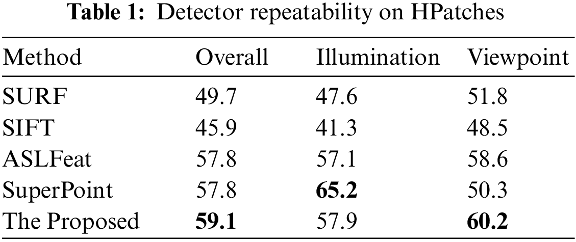
The result is shown in Fig. 3 and Tab. 1. In Fig. 3, The abscissa is the pixel-level error threshold from 1 pixel to 10 pixels, and the two rows from top to bottom represent MMA, M.S. under different error thresholds.

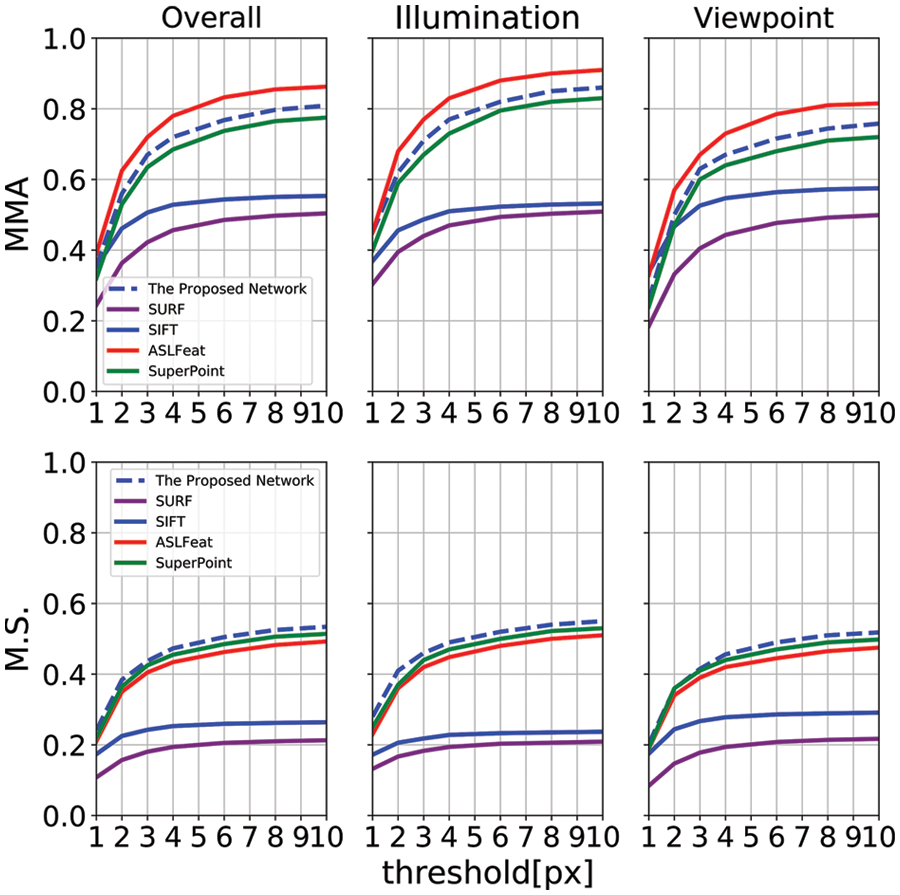
Figure 3: The comparison of the proposed network with the classical methods SIFT, SURF and the learning-based networks ASLFeat and SuperPoint on mean matching accuracy (MMA) and matching score (M.S.) on HPatches. The second and the third column indicates the situation with illumination changes only and random perspective changes only respectively. And the first column indicates the average error value of these two columns. The proposed network has the best performance on M.S. and has comparable results with the latest learning-based methods on MMA

Because of the excellent network architecture that keypoint detector and descriptor reorganizes the low-resolution feature maps of multiple layers to the original image resolution, which improving the accuracy of keypoint location and generating descriptors with rich local structure information. The proposed network outperforms SuperPoint and traditional feature extraction algorithm on all metrics. ASLFeat has the best performance on the MMA metric. In addition, it is clear that learning-based methods are significantly better than traditional methods on MMA and M.S.

The Keypoint repetition rate (REP%) mainly measures the performance of the detector. To measure the detection ability of the proposed network for keypoints, this paper also compares with SIFT, SURF, SuperPoint and ASLFeat on REP. In order to ensure fairness, NMS is all set to 4, and the error threshold is 3 pixels. The results are shown in Tab. 1. The proposed network performs the best on the branch of viewpoint change, and the overall performance is also the best.

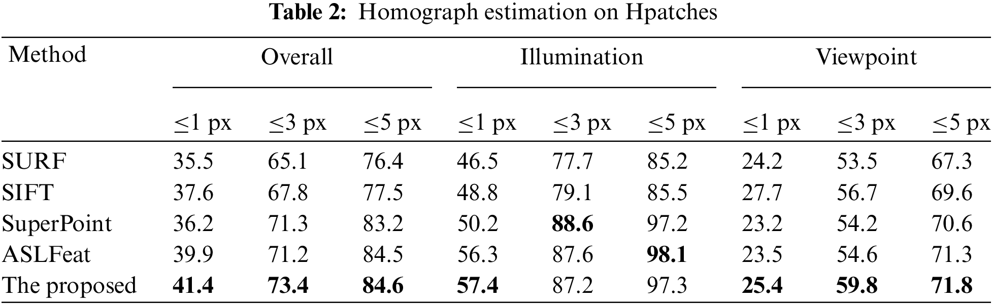
5.2 Homography Estimation on HPatches

The three metrics in Sec. 5.1 do not always reflect the geometric relationship between two images. For example, considering a case that a network detects only one keypoint with the same geometric content in each pair of images, and this pair of keypoints in the visible area in both pictures is judged to be a correct match. Then for this match, its MMA, MS and REP are all 1 (100%), which is actually meaningless, because the geometric relationship between these two pictures cannot be recovered by this match. For downstream tasks of image matching, such as SfM, it is usually necessary to find no less than 1000 pairs of precise matches between two images to robustly reconstruct 3D geometry. On the other hand, a relatively uniform distribution of keypoints is also important, but this is often difficult to measure directly [25,26]. Therefore, followings [16,27], this work uses H matrix estimation accuracy (HA%) to indirectly measure the accuracy and robustness of the network for finding connections between images.

5.2.1 Evaluation Protocols

It is not appropriate to directly calculate the similarity between the 3 × 3 true H and the estimated H', because different numbers in the H matrix have different scales. Referring to the method in [16], considering the four corner points in If, {kf1, kf2, kf3, kf4}, this paper uses the true H matrix to project it under the Is coordinate and obtain {ks1, ks2, ks3, ks4}, then uses the estimated homography transformation matrix H' [28] to get {ks1', ks2', ks3', ks4'}, finally calculates the distance between these four projected point pairs. If the distance is less than ε, it is judged that the estimate is correct. As shown in the formula:

HA=1N∑i=1N((14∑j=14||kij−kij′||)≤ε)(19)

This work compares the method proposed with the traditional feature detection and description algorithms SIFT, SURT, these two methods are implemented using OpenCV, and the latest learning-based methods: SuperPoint and ASLFeat. In order to ensure fairness, all methods are performed on the image size of 480×640. The feature matching algorithm using here is nearest neighbor algorithm. The H-matrix estimation is realized by OpenCV (findHomography ()). RANSAC is also used to enhance estimation accuracy. In addition, NMS = 4.

5.2.2 Comparisons with Other Methods

This work follows the practice of patch2pix [29] and reports the percentage of errors below 1, 3 and 5 pixels, as shown in Tab. 2. This work chooses the default settings of SURF and SIFT to apply them. For SuperPoint and ASLFeat, this work uses the settings reported in their respective papers. Firstly, similar to the results in Sec. 5.1, deep learning-based methods have made great progress over traditional methods. Secondly, the proposed method has the best performance on the branch of Viewpoint change and comprehensive performance, and it performs the best when the thresholds are 1 pixel and 3 pixels in both Illumination and Viewpoint changes, which shows that the proposed method improves the localization accuracy of keypoints. In particular, the improvement is obvious compared to SuperPoint, which again demonstrates the effectiveness of the proposed structure.

6  Conclusion

The quality and accuracy of image matching play a vital role in many computer vision tasks. In order to alleviate the problems of current feature extraction methods, this work designs a new convolutional neural network to jointly and intensively extract keypoints. On the one hand, the proposed network uses multi-level features to restore low-level details, thereby improving the positioning accuracy of keypoints. On the other hand, the proposed network utilizes multiple hierarchical features to generate robust keypoint descriptors. Detailed experiments on HPatches have confirmed the superiority of the proposed network against traditional methods and the learning-based approaches.

Funding Statement: This work was supported by the National Natural Science Foundation of China (61871046, SM, http://www.nsfc.gov.cn/).

Conflicts of Interest: The authors declare that they have no conflicts of interest to report regarding the present study.

This work is licensed under a Creative Commons Attribution 4.0 International License, which permits unrestricted use, distribution, and reproduction in any medium, provided the original work is properly cited.