Computers, Materials & Continua DOI:10.32604/cmc.2022.029604
Article

Big Data Analytics with Artificial Intelligence Enabled Environmental Air Pollution Monitoring Framework

Manar Ahmed Hamza1,*, Hadil Shaiba2, Radwa Marzouk3, Ahmad Alhindi4, Mashael M. Asiri5, Ishfaq Yaseen1, Abdelwahed Motwakel1 and Mohammed Rizwanullah1

1Department of Computer and Self Development, Preparatory Year Deanship, Prince Sattam bin Abdulaziz University, AlKharj, 16278, Saudi Arabia
2Department of Computer Sciences, College of Computer and Information Sciences, Princess Nourah bint Abdulrahman University, P. O. Box 84428, Riyadh, 11671, Saudi Arabia
3Department of Information Systems, College of Computer and Information Sciences, Princess Nourah bint Abdulrahman University, P. O. Box 84428, Riyadh, 11671, Saudi Arabia
4Department of Computer Sciences, College of Computing and Information System, Umm Al-Qura University, Saudi Arabia & Research and Innovation, Salla Holding Limited, Makkah, Saudi Arabia
5Department of Computer Science, College of Science and Arts, King Khalid University, Mahayil Asir, 62529, Saudi Arabia
*Corresponding Author: Manar Ahmed Hamza. Email: ma.hamza@psau.edu.sa
Received: 07 March 2022; Accepted: 06 April 2022

Abstract: Environmental sustainability is the rate of renewable resource harvesting, pollution control, and non-renewable resource exhaustion. Air pollution is a significant issue confronted by the environment particularly by highly populated countries like India. Due to increased population, the number of vehicles also continues to increase. Each vehicle has its individual emission rate; however, the issue arises when the emission rate crosses the standard value and the quality of the air gets degraded. Owing to the technological advances in machine learning (ML), it is possible to develop prediction approaches to monitor and control pollution using real time data. With the development of the Internet of Things (IoT) and Big Data Analytics (BDA), there is a huge paradigm shift in how environmental data are employed for sustainable cities and societies, especially by applying intelligent algorithms. In this view, this study develops an optimal AI based air quality prediction and classification (OAI-AQPC) model in big data environment. For handling big data from environmental monitoring, Hadoop MapReduce tool is employed. In addition, a predictive model is built using the hybridization of ARIMA and neural network (NN) called ARIMA-NN to predict the pollution level. For improving the performance of the ARIMA-NN algorithm, the parameter tuning process takes place using oppositional swallow swarm optimization (OSSO) algorithm. Finally, Adaptive neuro-fuzzy inference system (ANFIS) classifier is used to classify the air quality into pollutant and non-pollutant. A detailed experimental analysis is performed for highlighting the better prediction performance of the proposed ARIMA-NN method. The obtained outcomes pointed out the enhanced outcomes of the proposed OAI-AQPC technique over the recent state of art techniques.

Keywords: Sustainability; environmental air quality; predictive model; pollution monitoring; statistical models; artificial intelligence

1  Introduction

With the technological and economic improvement of cities, environmental pollution challenges are rising, like air, water, and noise pollution. Particularly, air pollution is a significant effect on human health over the disclosure of particulates and pollutants that has greater attention in air pollution and their effects amongst the academic research [1,2]. The major main cause related to air pollution comprises agriculture, burning of fossil fuels, natural disasters, residential heating, exhaust from industries and factories.

Recently, the Internet of Things (IoT) model has developed, enabling objects of daily lives with transceivers for digital communication, a suitable protocol stack, and microcontrollers empowers them to interact with each other, becomes an essential component of the Internet. Because of this accumulation, devices like surveillance cameras, home appliances, vehicles, and sensors could produce large numbers of data which could be consequently analyzed and utilized for developing novel applications. The current advancement in IoT techniques has enabled persons to improve effective systems consists of WiFi/Bluetooth for near regions, satellites for remote regions and mobile networks, multiple sensors connected wirelessly for monitoring distinct air pollutants in various fields. Such amount of data may require parallelization utilizing cloud computing and big data technique for facilitating nearby real-world monitoring [3] and analyzing evolving patterns.

The monitoring system allows gathering quality data that could be utilized for extracting deeper knowledge on pollution [4]. Air pollution predicting system enables to forecast the Air Quality Index (AQI), the values of pollutant, like carbon dioxide concentration (i.e., PM2.5, PM10, CO2, etc) or particle matter (PM), and identify higher pollution regions. Prediction air pollution system could assist government employs smart solutions and precautions for addressing air quality issues. Even though several models and solutions for forecasting air pollutions were introduced in the study, usually they are categorized into 2 classifications. Firstly, it tracks the transmission, generation, and dispersion processes of pollutants. The mathematical simulation generates the prediction result of this model. Next, it consists of deep learning (DL), statistical learning, and machine learning (ML) methods [5].

The current study shows that the conventional deterministic method struggles for capturing the nonlinear relations among the focuses of contaminant and their sources of dispersion and emission [6], particularly in a model application in region of complicated environment. In order to address the limitation of conventional method, the most significant method is to utilize statistical model on the basis of ML methods. Statistical methods do not consider the chemical and physical procedures and utilize past data for predicting air quality. Methods were trained on present measurement and utilized for estimating or forecasting concentration of air pollutants based on the prediction features (such as land use, meteorology, human activity, time, planetary boundary layer, elevation, pollutant covariates, and so on.). The simple statistical approach includes Time Series, Autoregressive Integrated Moving Average (ARIMA), and Regression model. Such analysis determines the relations among parameters according to the possibility and statistical average. Well stated regression could give moderate results. But, the reactions among influential factors and air pollutants are nonlinear, leads to complicated systems of air pollutant formation mechanism. Hence, more innovative statistic learning (or ML) approaches are desirable to account for accurate nonlinear modeling of air pollution. Such as, Ensemble Learning, Support Vector Machines (SVM), and Artificial Neural Networks (ANN) were employed to conquer nonlinear uncertainties and limitations for achieving an optimal predictive accuracy. Even though statistical methods don’t explicitly simulate the environment process, they usually exhibit a high prediction efficiency compared to CTM on fin spatio-temporal scales in the existence of wide monitoring data [7].

In the application of big data services and technology in the procedure of ecological civilization construction and current environment protection, they could moderately utilize big data for solving few complex challenges in environment protection works 1) data collection and disclosure; 2) air quality prediction and earlier warnings; 3) utilizing big data acquisition technique for annualizing the cause of environmental pollution. The data analyses activity is performed by integrating different kinds of emission information of pollution sources and environment indicators. Using moderate prediction and scientific analysis of enterprise sewage intensity, its impacts on the surrounding environmental quality, and distribution of pollution sources, the environment treatment proposal is developed, and the impact of environment treatments is regularly monitored, and the treatment plans are continuously improving. The application and development of big data techniques could be stated to offer a novel method for humans to handle environmental challenges [8]. For environmentalists, it is essential to actively promoting the reasonable application of big data techniques in the region of environment protection, in order to obtain more independence in understanding the objective law of natural developments.

This study develops an optimal AI based air quality prediction and classification (OAI-AQPC) model in big data environment. To manage the big data from environmental monitoring, Hadoop MapReduce tool is used. Moreover, a hybridization of ARIMA and neural network (NN) called ARIMA-NN is designed to predict the pollution level, and the parameters in the AIMA-NN model are tuned by the use of oppositional swallow swarm optimization (OSSO) algorithm. At last, Adaptive neuro-fuzzy inference system (ANFIS) classifier is used to classify the air quality into pollutant and non-pollutant. The use of ARIMA-NN technique is utilized for predicting the air quality parameters and the ANFIS technique is employed to categorize the air quality into pollutants and non-pollutants depicts the novelty of the study. A wide range of simulation analyses is carried out and the results are inspected interms of different dimensions.

2  Literature Review

Kalajdjieski et al. [9] proposed a new methodology calculating 4 distinct frameworks which exploit camera images to evaluate the air pollution in this region. The projected method utilizes generative adversarial network and data augmentation methods for mitigating class imbalance problems. In Ghaemi et al. [10], a spatio-temporal method is proposed by a LaSVM based online approach. Meteorological data, geographical, Pollutant concentration parameters are repeatedly fed into the advanced online predicting method. The efficiency of the scheme is calculated by relating the predictive result of the AQI with conventional SVM method. Zhang et al. [11] proposed a predictive approach integrating Long Short-Term Memory networks (LSTM) and Graph Attention (GAT) model. In this case, the LSTM is utilized for defining the temporal correlation of historical data and GAT is applied to represent the spatial correlation amongst all the monitoring stations in the destination.

Honarvar et al. [12], developed a prediction method for PM predictions. The presented method contains many elements for integrating heterogeneous multiple sources of urban data and forecast the particulate matter according to the TL point of view, where regression and NN were leveraged as the heart of predictions. The result of the particulate matter predictions revealed that data sources can able to predict accurate particulate matter. Zaree et al. [13] aim is to raise accuracy and speed in predicting location, effects of weather conditions on density of air pollution, and real levels of air pollution, a K-means clustering method with Mahout library is utilized as a big data mining tool on data sets of a city pulse project.

Shahbaz et al. [14] explored the new phenomenon of a BDA-EAP management scheme and presented a study of factors affecting adaption of this scheme. This study is depending on a TTF and unified concept of acceptance and UTAUT concept. A complete BDA-EAP management scheme is presented and the possible adaption speed of this scheme is calculated by transmitting structured forms to the employees of appropriate environment agency, yield 412 valid replies, utilizing structural equation modelling method. Al-Janabi et al. [15] designed a smart predictor for the concentration of air pollutants on the following 2 days relying on DL method utilizing RNN. The optimal structure for its process is later defined by a PSO method. The novel predictor dependent smart computation is based on unsupervised learning, viz., LSTM and optimization (viz., PSO) is known as SAQPM.

Shih et al. [16] proposed a PM2.5 instant predictive framework based on Spark big data architecture for handling large data from the LASS community. The Spark big data architecture presented in the research is separated into 3 models. The simulation result shows that the presented Spark big data ensemble predictive method in following 30-min predictions has an optimal efficiency (R2 up to 0.96), and the ensemble method has higher efficiency compared to individual ML method. Castelli et al. [17] employ a common ML technique, SVR, to predict particulate and pollutant levels and to forecast the AQI. Amongst the different tested alternates, RBF was the kind of kernel which allows SVR for obtaining the precise prediction. Utilizing the entire set of available parameters exposed an effective approach compared to FS utilizing PCA.

Chang et al. [18] proposed a semantic ETL architecture on cloud environment for predicting AQ. In the environment, they exploit ontology for concretizing the relation of PM 2.5 from different data sources and to combine such data with a similar idea but distinct naming to the unified database. They implemented the ETL architecture on the cloud environment that consists of storage nodes and computing nodes. In Zou et al. [19], an AQI predictive method (i.e., airQP-DNN) and its application are projected for addressing this problem. Primarily, this study contains 2 modules. The initial module is to forecast the upcoming AQI on the basis of DNN, weather predicting datasets, present meteorological datasets, and using historical air quality datasets. Next, it refers to an analysis of outdoor events route planning in Beijing, that could assist plan the routes for outdoor events according to the air using QP-DNN method, and allows users to enter the source and end point of the routes for the optimized path using a minimal collected AQI.

3  The Proposed Model

This study has devised a new OAI-AQPC technique to predict and classify air quality in the big data environment. The proposed model involves Hadoop Map Reduce tool to manage big data. As demonstrated in Fig. 1, the workflow of the OAI-AQPC technique encompasses different processes namely ARIMA-NN based prediction, OSSO based parameter optimization, and ANFIS based classification. The use of ARIMA-NN technique is utilized for predicting the air quality parameters and the ANFIS manner is employed to categorize the air quality into pollutants and non-pollutants. The detailed working of these processes is elaborated in the subsequent sections.

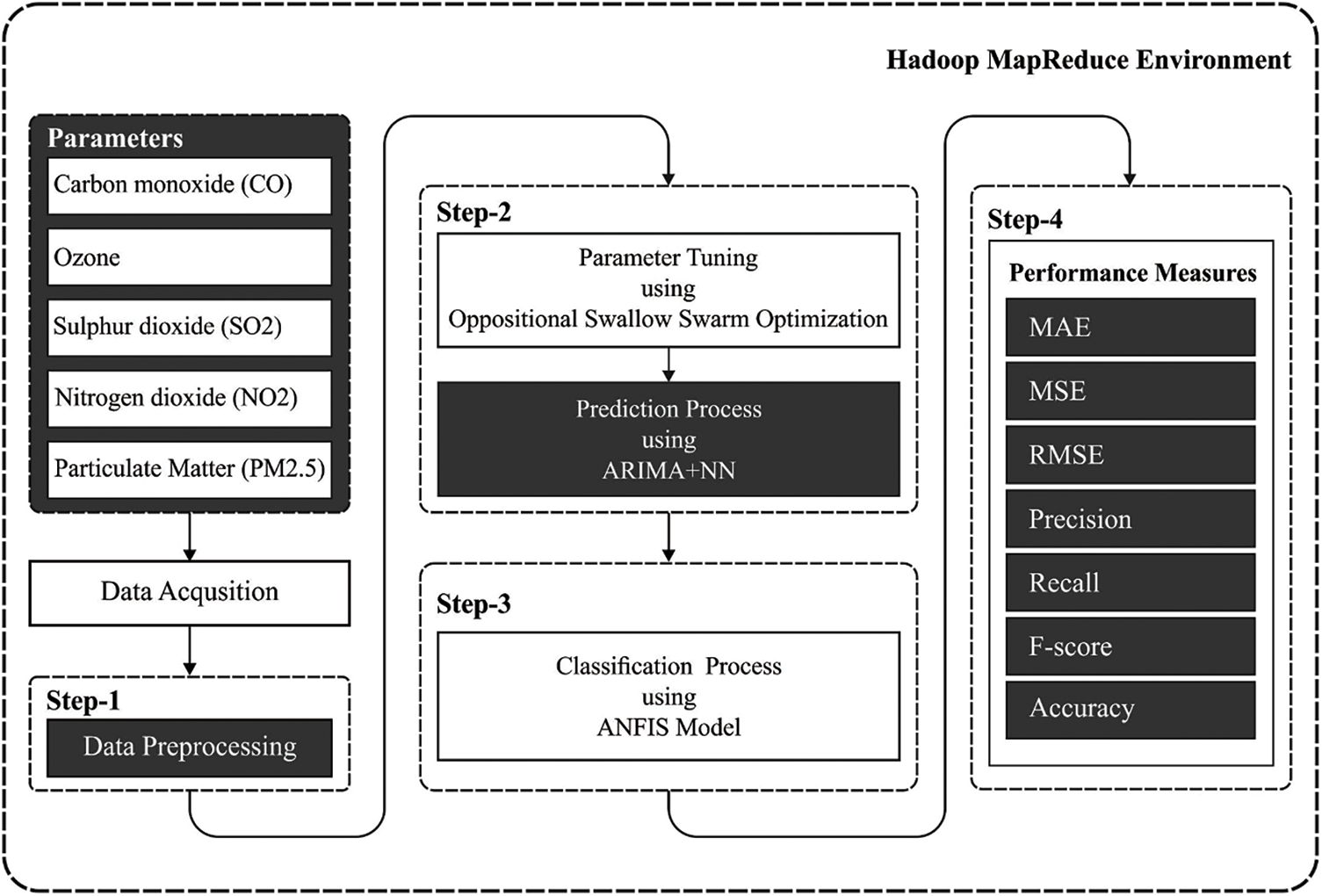
Figure 1: Overall process of OAI-AQPC model

3.1 Framework of Hadoop Map Reduce Model

The MR runtime environment is one of popular models utilized in the distributed processing system. As privative tool, its open-source counterpart, called Hadoop, was conventionally utilized in study field [20]. It was proposed for allowing distributed computation in an apparent manner for the programmer, as well as provide automated data partition and management, automatic job/resource scheduling, and fault tolerance. For using this system|, another process should be separated into 2 major phases: Reduce and Map. Firstly, it is dedicated to splitting the data to process, while the next one aggregates and collects the result. Moreover, the MR method is determined based on a fundamental data structure: the (key, value) pairs. The processing data, the intermediate and final result works based on (key, value) pair. For summarizing this process, Fig. 2 shows a usual MR program with its Map and Reduce phases. The MR system could be defined in the following.

•   First, the map function reads information and transforms records to a key value format. Transformation in this stage might employ any series of operations on every record beforehand transmitting the tuples through the network.

•   Then, the output key is grouped and shuffled with a key value thus equivalent keys are gathered for creating a list of values. Later, Keys are divided and transmitted to the Reducer based on some key based system determined before.

•   Lastly, the reducer performs this fusion on the list for ultimately generating an individual value for all pairs. As a new optimization, the reducers are also utilized as a combiner on the map output.

The enhancement decreases the overall number of data transmitted through the network by integrating every word created in the Map phase to an individual pair. Besides, taking into account MR as a processing model, this system could be viewed as a fusion procedure which permits merging information schemes and partial models to a final fused result. Fusion of methods in MR has usually executed this ensemble approach which integrates various hypotheses via attachment/voting. As well, another proposal exists that exceeds ensemble learning, and provide result as an individual coalesced method. As logistic regression in Spark is made up of various subgradients that are eventually aggregated and locally computed.

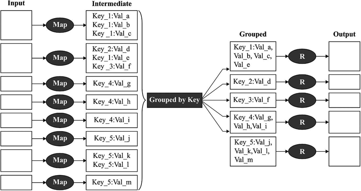
Figure 2: Framework of MR model

3.2 Prediction using ARIMA-NN Model

Primarily, the hybridization of ARIMA and NN takes place for the prediction of the pollution level in the environment. The ARIMA is initially proposed by Box and Jenkin in 1976. A common formula of successive variances at dth variance of Xt is given as follows:

ΔdXt=(1−B)dXt(1)

where d implies the variance order and is generally 1 or 2, and B represents the backshift operator. The following variance at one-time lag is equivalent to,

Δ1Xt=(1−B)Xt=Xt−Xt−1(2)

During this case, a common ARIMA (p,d,q) is written as follows [21]:

Φp(B)Wt=θq(B)et(3)

where Φp(B) refers the auto-regressive operator of direction p, θq(B) is a moving average operator of order q, and Wt=ΔdXt.

The ARIMA model efficiency is estimated utilizing root mean square errors (RMSEs, Eq. (4)) and coefficient of resolve (R2).

RMSE=∑i=1n(Xt−X0)2n(4)

where Xt signifies the estimated observation and X0 refers the actual observation.

Amongst several NN frameworks, the feedforward BP network is mostly utilized. This network framework contains single hidden layer of neurons using a non-linear transfer function and an output layer of linear neurons using a linear transfer function. In the BP networks, xj=1,..,N denotes the input parameters; ni(i=1,…,S) signifies the output of neurons in the hidden layer and yt (t=1,…L) indicates the output of NN. A NN should be trained for determining the values of weight that would generate the accurate output. In the training stage, a group of input data is utilized to train and present to the network several times. The efficiency of the network is tested afterward the training phase is ended. It is the direction where the efficiency function is reducing more quickly. It turned out that even though the function reduces more quickly with the negative of the gradient, it doesn’t generate faster convergence [22]. Thus, the fundamental gradient descent training approach is ineffective because of its slower convergent speed and poor accuracy in prediction method. From an optimization perspective, training a NN could be deliberated as equal for minimizing a multi-variable global error function of the network weight. The SCG method was established for avoiding the time-consuming line search. The conventional BP method, usually applied in NN learning, calculates the gradient of global error function regarding the weights, (Wk), at all iterations and update the weight based on

Wk+1=Wk−αk∇f(Wk)(5)

The step size αk>0 represents a user-selected learning rate parameter that affects the efficiency of learning process to a large amount. In each case, the BP approach might follow a zigzag path to the minimal, usual for a steepest gradient descent technique. In case Dk denotes the direction vector at iteration k, then the weight vectors are upgraded based on

Wk+1=Wk+αkDk(6)

The assumed values of Wk and Dk, certain values of αk reduces the objective function more rapidly, which must be established. The evaluation of the optimal step size along SCG training method rises the learning speed and removes the dependency on crucial user-selected parameters. The major concept behindhand the process is the utilization of a factor ρ i.e., lowered/raised within all iterations at the time of implementation, look at the symbol of quantity δ exposes when the Hessian matrix isn’t positive definite. The summary of SCG in NN is provided in following [23].

     i)  Initialization: At k=0, select a primary weight vector W∘, and fix the primary direction vector to the negative gradient vector Do=Go=−∇f(Wo). fix the scalar 0<σ<10−4,0<ρ0≤10−6, ρ¯o, fix the boolean success =true.

    ii)  in case of success = true, evaluate next order data: σk=σ|Dk|, Sk=∇f(Wk+σkDk)−∇f(Wk)σk, δk=transpose (Dk)+Sk

   iii)  Scale δk:δk=δk+(ρk−ρ¯k)|Dk|2, looking at the sign of δk for all iterations altering ρk. When δk≤0, ρk & Sk is evaluated again.

    iv)  When δk≤0 create the Hessian positive definite

     v)  ρ¯=2(ρk−δk/|Dk|2), δk=−δk+ρk|Dk|2, ρk=ρ¯k

    vi)  Evaluate the step size: ξk=trcmspose(Dk)Gk, αk=ξk/δk, the value of ρk directly measure the step size, bigger the ρ small the step size.

   vii)  Evaluate relation parameters ck:ck=2δk⌊f(Wk)−f(Wk+αkDk)⌋/(ξk)2

  viii)  Weight and direction upgrade: When ck≥0, a success upgrade could be done: Wk+1=Wk+αkDk,Gk+1=−∇f(Wk+1), ρ¯k=0, success =true. When k modN=0 resume the process using Dk+1=Gk+1 else βk=(|Gk+1|2−Gk+1TGk)/ξk,Dk+1 =Gk+1+βkDk. If ck≥0.75 reduces the scale variable to ρk=14ρk else ρ¯=ρ success =false.

    ix)  When ck≥0.25 rise the scale variable to ρk=ρk+δk(1−ck)/|Dk|2

     x)  Repetition: when the steepest descent direction Gk≠0, set k=k+1 and return to step 2 otherwise end and return Wk+1 as minimal.

3.3 Design of ARIMA-NN Model

The performance of air quality can be predicted using the OAI-AQPC technique. The estimation of the ARIMA model to complicate non-linear problems might not be sufficient. Alternatively, utilizing ANN for modeling linear problems has produced insufficient outcomes. A hybrid method containing nonlinear and linear modelling capabilities can be a better alternative to predict air quality data. With the integration of distinct methods, various features of fundamental patterns might be taken. Next, in hybrid method, the air quality time sequence can be made up of a linear nonlinear component and auto relation structure.

yt=Lt+St(7)

where Lc denotes the linear element and St signifies the nonlinear element. Those variables should be evaluated from the time sequence data. Firstly, the ARIMA method is utilized for capturing the linear element, later the residual from the linear method would have the nonlinear relation. The residual et at time t from the linear method is determined as follows

et=yt−L^t(8)

where L^t denote the predictive values of ARIMA method at time t. The analytic check of the residual is significant for determining the sufficiency of ARIMA model. ARIMA models are not adequate when there is still linear relation structure remain in the residual. But, analytic check of the residual isn’t capable of detecting nonlinear patterns in the time's sequence data. Therefore, though the residual passes the analytic check and the models are a sufficient one, still the method mightn’t be sufficient because nonlinear relations haven’t been modelled properly. Thus, the residual could be modelled with the help of ANNs for discovering nonlinear relationships. Using N input node, the ANN method for the residual would be given as

et=f(et−1,et−2,….,et−N)+εt(9)

whereas f denotes a nonlinear function defined using a NN and εt represents the arbitrary error. Lastly, the integrated predictions would be

y^t=L^t+S^t(10)

where S^t denotes the prediction from Eq. (9).

3.4 Parameter Tuning using OSSO Algorithm

For enhancing the predictive efficiency of the AIRMA-NN model, the parameter tuning process gets executed by the use of OSSO algorithm. The SSO technique simulated as the combined effort of swallow and the interface amongst flock members has gained optimum outcomes. This technique was projected a metaheuristic approach dependent upon special properties of swallows are comprising fast flight, hunting skill, and intelligent social relation. At a glance, this technique has same as PSO but it can be unique features that could not be initiate in same techniques are containing the utilize of 3 kinds of particles: Explorer Particles (ej), Aimless Particles (oi), and Leader Particles (li), every of that is certain responsibility in the group. The ej particle is responsible to search the problem space. It can be carried out this exploring performance in the control of the number of parameters [24]. The particles utilize the subsequent formulas to explore and continue the path:

VHLi+1=VHLj+αHLrand()(ebest−ej)+βHLrand()(HLj−ej)(11)

Eq. (11) illustrates the velocity vector variable in the path of global leaders.

αHL={if(ej=0||ebest=0)−−>1.5}(12)

Eqs. (12) and (13) compute the acceleration coefficients variable (αHL) that directly impacts individual experience of all particles.

αHL={if (ei<ebest)&&(<HLi)→rand()⋅eiei⋅ebestei,ebest≠0if (ei<ebest)&&(ei>HLi)→2rand()⋅ei1(2⋅ei)ei≠0if (ei>ebest)→ebest1(2⋅rand())(13)

βHL={if(ej=0||ebest=0)−−>1.5}(14)

βHL={if(ei<ebest)&&(ei<HLi)→rand()⋅eiei⋅HLiei,HLi≠0if(ei<ebest)&&(ei>HLi)→2rand()⋅ei1(2⋅ei)ei≠0if (ei>ebest)→HLi1(2⋅rand())(15)

Eqs. (14) and (15) computes the acceleration coefficient variables (βHL) that directly affects the combined experiences of all particles. Actually, these 2 acceleration coefficients are quantified allowing for the place of all particles relative to optimum individual experience and global leaders. The oi particles utilize the subsequent Eq. (16) for arbitrary movements:

oi+1=oi+[rand({−1,1})∗rand(mins,maxs)1+rand()](16)

In SSO technique, there are 2 kinds of leaders: the local as well as global leaders. The particles are separated as to groups. The particles in all groups are frequently same. Afterward, an optimum particle in all groups is elected and is named as local leader. Then, an optimum particle amongst the local leaders is selected and is named as global leader. The particle alteration its way and converge based on place of these particles.

To enhance the convergence rate of the SSO algorithm, the OSSO algorithm is designed by the incorporation of OBL concept. It performs by exploring all directions in the search space namely actual and opposite solutions. The opposite number x is defined as a real number in the range of x∈[lb,ub]. The opposite number of x is represented by x~ [25]:

x~=lb+ub−x(17)

To generalize it, every searching agent and the opposite solution is represented as follows.

x=[x1,x2,x3,…xD](18)

x~=[x~1,x~2,x~3,…,x~D](19)

The value of all the components in x~ can be represented using Eq. (20):

x~j=lbj+ubj−xjwhere j=1,2,3,…,D(20)

If the fitness value f(x~) of the opposite solution exceeds the f(x) of the original solution x, then x=x~; else x=x.

3.5 ANFIS Based Classification

Once the air quality is predicted by the ARIMA-NN technique, the next stage involves the classification of air quality parameters into pollutants and non-pollutants using the ANFIS classifier. The ANFIS model integrates the processing ability of the ANN and high-level logical ability of the FIS technique. Alternatively, the ANFOS model is derived by adding the FIS into the adaptive network model. Due to the proficient learning and reasonability ability of the ANFIS technique, it is employed for the classification of air pollution monitoring in this study [26]. It comprises different characteristics which help to accomplish improved performance. The ANN model can determine the patterns by adapting to the platform with the learning abilities. In addition, the FLS technique integrates the expert’s opinion to make decisions. The capability of handling past data and expert opinion makes it adaptable to unusual situations. It is called an intelligent model due to the variables and fuzzy rules involved that are determined by the ANN model in an intelligent way.

4  Performance Validation

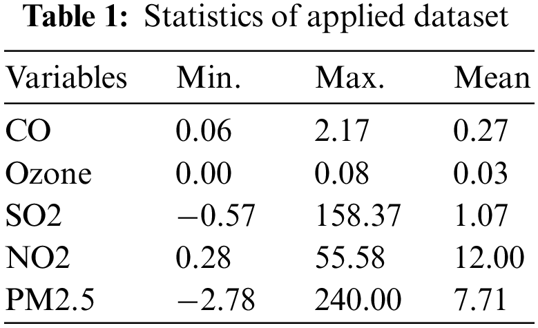
This section inspects the predictive and classification results analysis of the OAI-AQPC technique. The OAI-AQPC technique is simulated using Python 3.6.5 tool. The OAI-AQPC technique is validated using a dataset comprising different air quality parameters such as Carbon monoxide (CO), Ozone, Sulphur dioxide (SO2), Nitrogen dioxide (NO2), and Particulate Matter (PM2.5). The dataset holds a total of 22321 instances. The AQI values are grouped into 6 different classes as shown in Fig. 3. In addition, the good and moderate values come under ‘Non-Pollutant’ class (15738 instances) and the remaining values come under ‘Pollutant’ class (6583 instances). Besides, the statistical values of the dataset are given in Tab. 1.

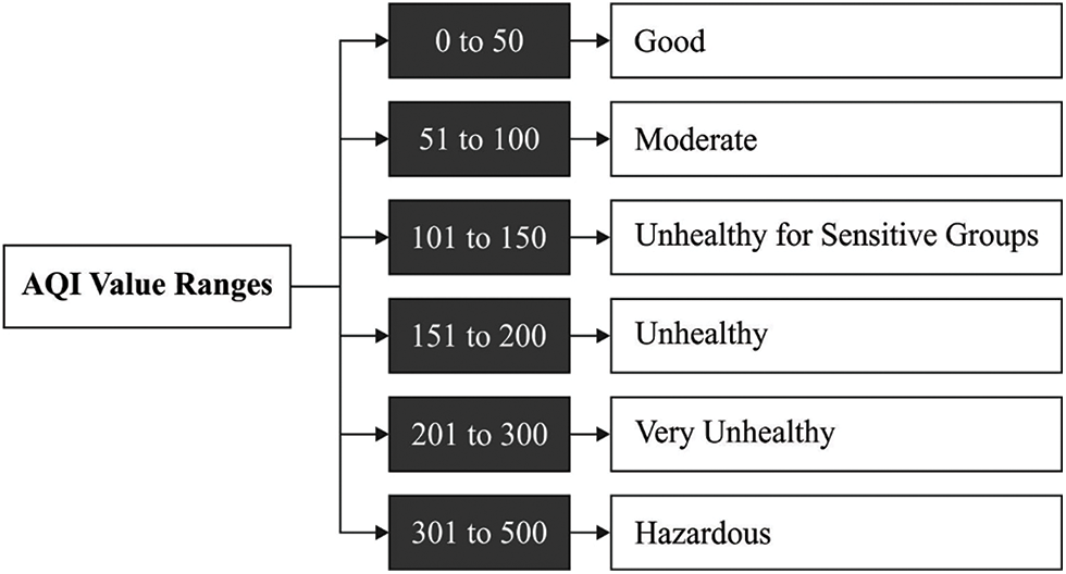
Figure 3: Six different classes

A brief forecasting results analysis of the ARIMA-NN technique is examined in Tab. 2 and Fig. 4 under varying training and validation sets. From the results, it is ensured that the ARIMA-NN technique has forecasted the variables effectively with the minimum MSE, MSE, and RMSE values. For instance, the ARIMA-NN technique predicted the ‘CO’ variable with the lower RMSE of 0.170 and 0.490 on the applied training and validation sets respectively. In addition, the ARIMA-NN approach predicted the ‘Ozone’ variable with the minimum RMSE of 0.105 and 0.247 on the applied training and validation sets correspondingly. Along with that, the ARIMA-NN manner predicted the ‘SO2’ variable with the lesser RMSE of 0.363 and 0.732 on the applied training and validation sets correspondingly. Moreover, the ARIMA-NN method predicted the ‘NO2’ variable with the least RMSE of 0.134 and 0.300 on the applied training and validation sets respectively. At last, the ARIMA-NN methodology forecast the ‘PM2.5’ variable with the minimal RMSE of 0.170 and 0.490 on the applied training and validation sets correspondingly.

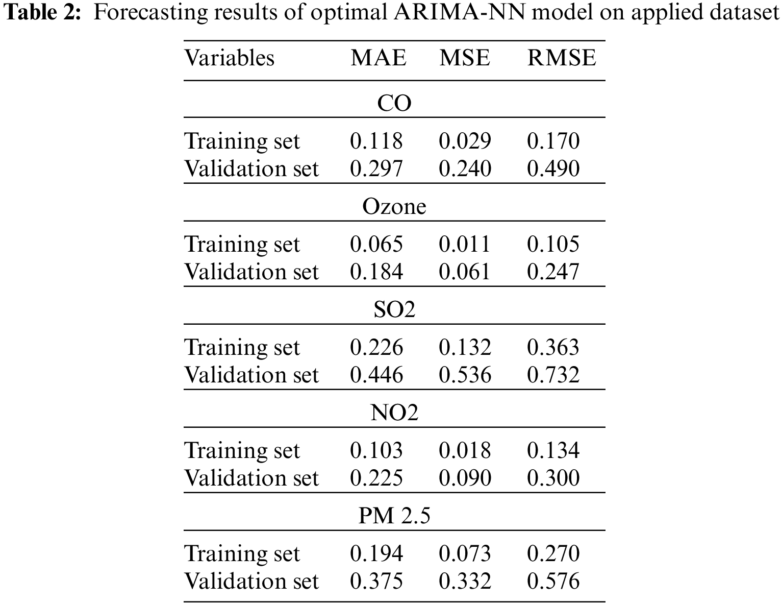
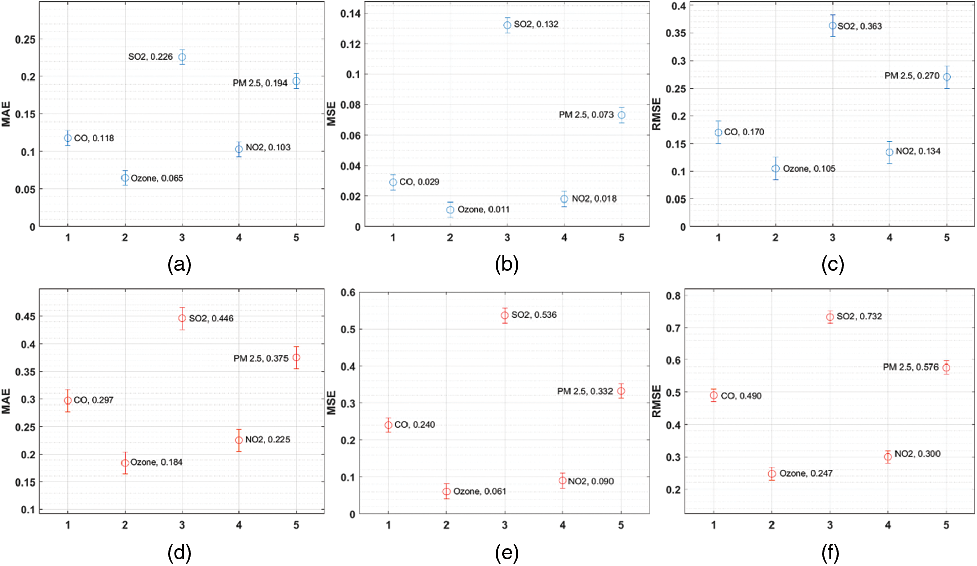
Figure 4: (a–c) Training set, (d–f) Validation set: Result analysis of ARIMA-NN model with different measures

Fig. 5 demonstrates the set of five confusion matrices produced by the OAI-AQPC technique under five distinct runs. Fig. 5a depicts the confusion matrix of the OAI-AQPC technique under the execution of run-1. The figure exhibited that the OAI-AQPC technique has classified the 13337 instances into Not Polluted class and 5983 instances into Polluted class. Simultaneously, Fig. 5b showcases the confusion matrix of the OAI-AQPC approach under the execution of run-2. The figure demonstrated that the OAI-AQPC manner has classified the 13537 instances into Not Polluted class and 5975 instances into Polluted class. Concurrently, Fig. 5c illustrates the confusion matrix of the OAI-AQPC manner under the execution of run-3. The figure outperformed that the OAI-AQPC technique has classified the 13458 instances into Not Polluted class and 6081 instances into Polluted class. In the meantime, Fig. 5d portrays the confusion matrix of the OAI-AQPC methodology under the execution of run-4. The figure demonstrated that the OAI-AQPC method has classified the 13698 instances into Not Polluted class and 6073 instances into Polluted class. Lastly, Fig. 5e illustrates the confusion matrix of the OAI-AQPC method under the execution of run-5. The figure showcased that the OAI-AQPC manner has classified the 13755 instances into Not Polluted class and 6103 instances into Polluted class.

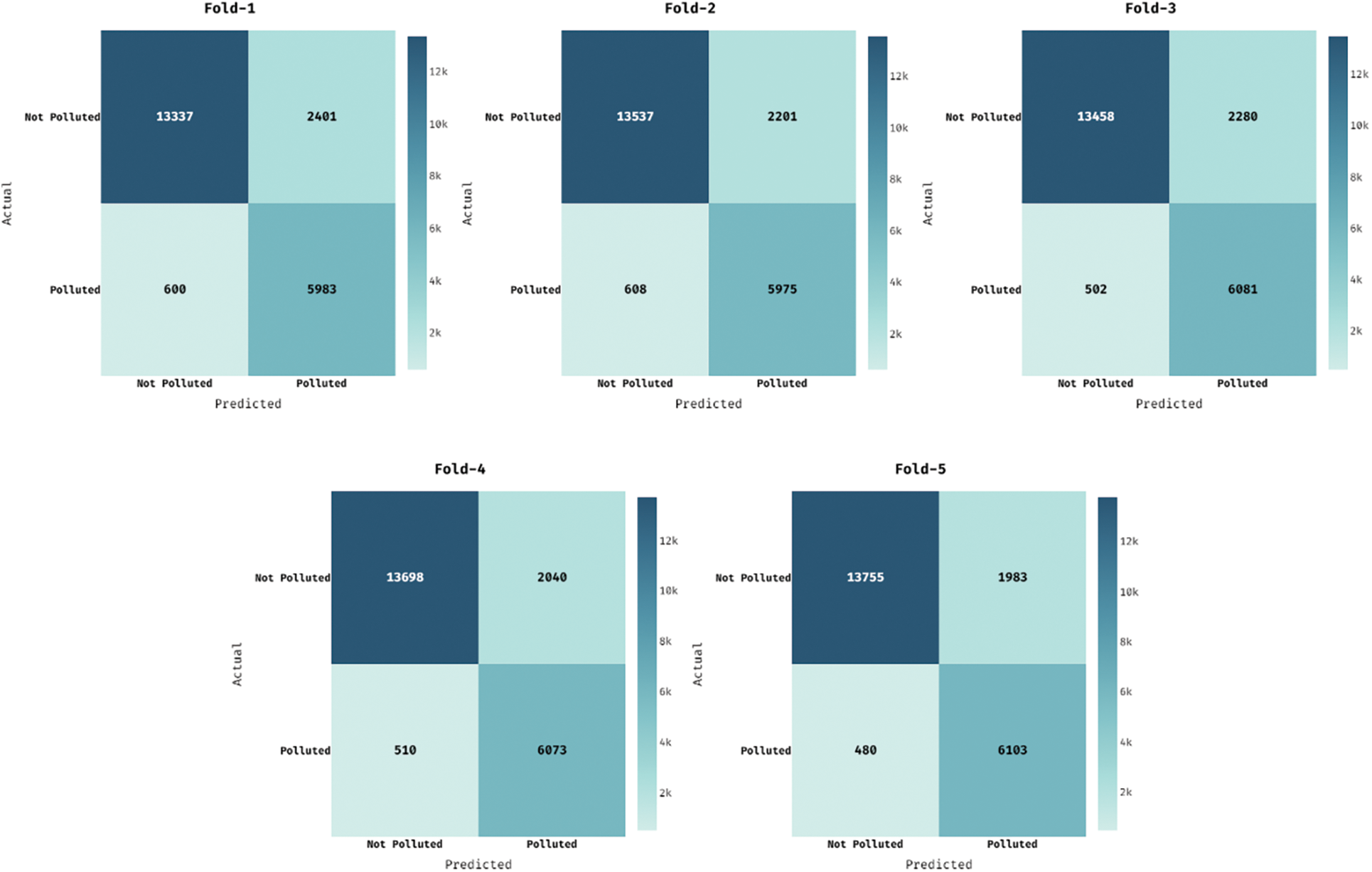
Figure 5: Confusion matrices of OAI-AQPC method

Tab. 3 and Fig. 6 offer the classification results analysis of the OAI-AQPC technique interms of different measures. From the table, it is demonstrated that the OAI-AQPC technique has gained effective classification outcomes on the applied dataset. For instance, under fold-1, the OAI-AQPC technique has obtained a precision of 0.982, recall of 0.963, accuracy of 0.962, and F-score of 0.972.

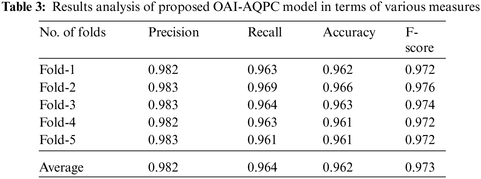
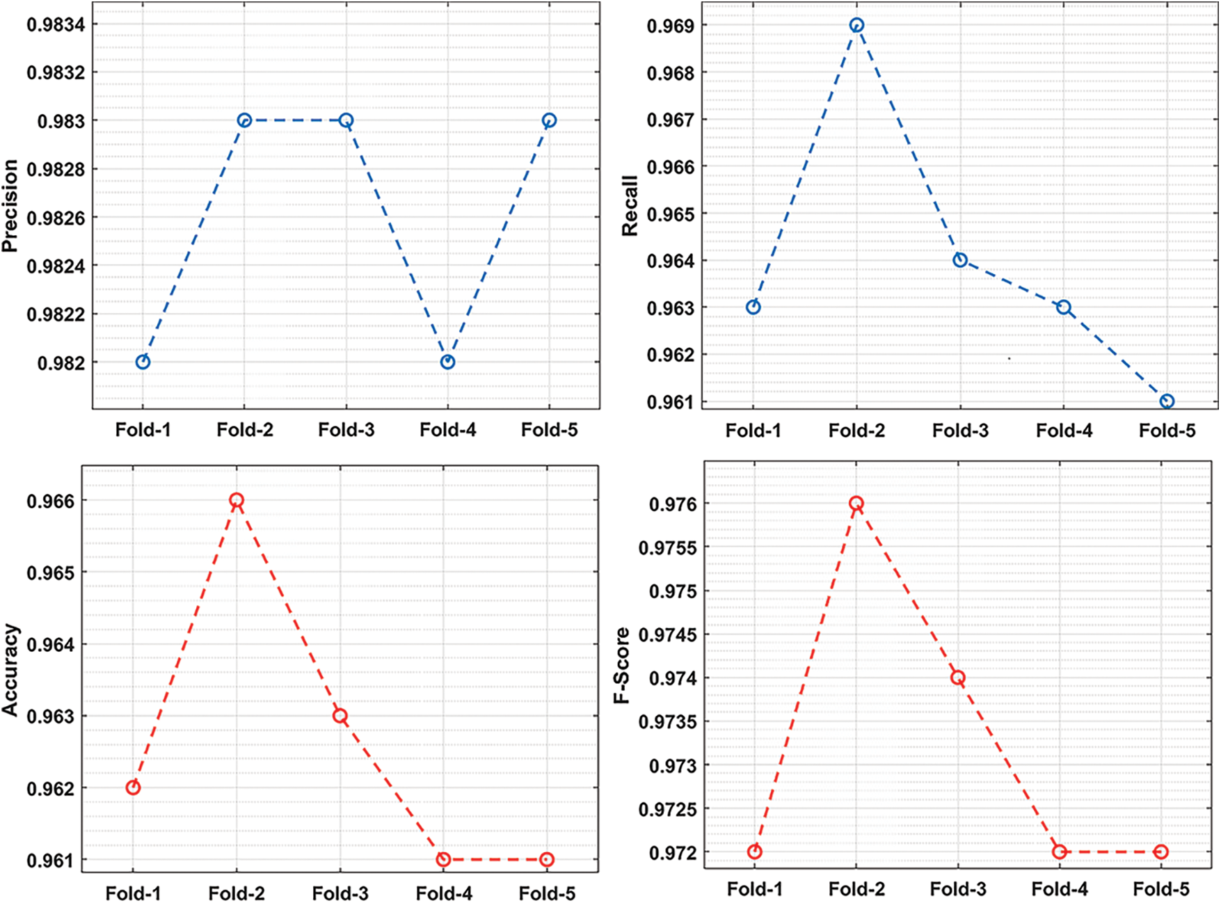
Figure 6: Classification results analysis of the OQI-AQPC technique

Also, under fold-2, the OAI-AQPC approach has gained a precision of 0.983, recall of 0.969, accuracy of 0.966, and F-score of 0.976. Additionally, under fold-3, the OAI-AQPC attained has achieved a precision of 0.983, recall of 0.964, accuracy of 0.963, and F-score of 0.974. Moreover, under fold-4, the OAI-AQPC methodology has gained a precision of 0.982, recall of 0.963, accuracy of 0.961, and F-score of 0.972. Furthermore, under fold-5, the OAI-AQPC methodology has gained a precision of 0.983, recall of 0.961, accuracy of 0.961, and F-score of 0.972.

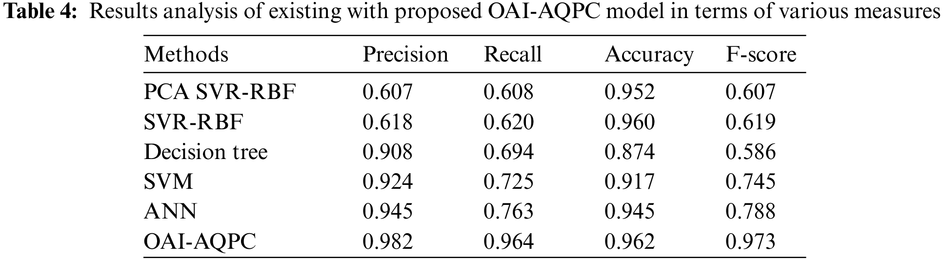
In order to guarantee the supremacy of the OAI-AQPC technique, a detailed comparison study is made in Tab. 4 [17]. The obtained results exemplified that the DT approach has showcased poor outcomes with the least accuracy of 0.874 whereas the SVM model has gained somewhat enhanced performance with an accuracy of 0.917. In addition, the ANN and PCA SVR-RBF techniques have showcased moderately closer outcomes with the accuracy of 0.945 and 0.952. Besides, the SVR-RBF technique has resulted in a near optimal outcome by offering high accuracy of 0.960. However, the proposed OAI-AQPC technique has depicted better performance over the other algorithms with maximum precision of 0.982, recall of 0.964, accuracy of 0.962, and F-score of 0.973.

From the above mentioned tables and figures, it can be stated that the OAI-AQPC technique has been found to be an appropriate air quality prediction and classification in the real time environment.

5  Conclusion

This paper has introduced an effective OAI-AQPC technique to predict and classify air quality on big data platforms. The OAI-AQPC technique encompasses different processes namely ARIMA-NN based prediction, OSSO based parameter optimization, and ANFIS based classification. The use of ARIMA-NN technique is utilized for predicting the air quality parameters and the ANFIS approach is employed to categorize the air quality into pollutants and non-pollutants. Besides, the application of OSSO algorithm to optimally adjust the parameters of the ARIMA-NN technique also results in improved air quality predictive outcomes. A wide range of simulation analyses is carried out and the results are inspected interms of different dimensions. The simulation values showcased the better performance of the OAI-AQPC technique over the other state of art predictive models interms of different evaluation parameters. In future, the performance of the OAI-AQPC technique is extended to the design of deep learning architectures for prediction and classification purposes.

Funding Statement: The authors extend their appreciation to the Deanship of Scientific Research at King Khalid University for funding this work under grant number (RGP2/45/43). Princess Nourah bint Abdulrahman University Researchers Supporting Project number (PNURSP2022R135), Princess Nourah bint Abdulrahman University, Riyadh, Saudi Arabia. The authors would like to thank the Deanship of Scientific Research at Umm Al-Qura University for supporting this work by Grant Code: (22UQU4270206DSR02).

Conflicts of Interest: The authors declare that they have no conflicts of interest to report regarding the present study.

This work is licensed under a Creative Commons Attribution 4.0 International License, which permits unrestricted use, distribution, and reproduction in any medium, provided the original work is properly cited.