Computers, Materials & Continua DOI:10.32604/cmc.2022.029619
Article

A Sea Ice Recognition Algorithm in Bohai Based on Random Forest

Tao Li1, Di Wu1, Rui Han2, Jinyue Xia3 and Yongjun Ren4,*

1School of Artificial Intelligence/School of Future Technology, Nanjing University of Information Science and Technology, Nanjing, 210044, China
2Unit 93117 of PLA, PLA, Jiangsu, 210000, China
3International Business Machines Corporation (IBM), NY, 100014, USA
4School of Computer Science, Nanjing University of Information Science and Technology, Nanjing, 210044, China
*Corresponding Author: Yongjun Ren. Email: renyj100@126.com
Received: 08 March 2022; Accepted: 07 May 2022

Abstract: As an important maritime hub, Bohai Sea Bay provides great convenience for shipping and suffers from sea ice disasters of different severity every winter, which greatly affects the socio-economic and development of the region. Therefore, this paper uses FY-4A (a weather satellite) data to study sea ice in the Bohai Sea. After processing the data for land removal and cloud detection, it combines multi-channel threshold method and adaptive threshold algorithm to realize the recognition of Bohai Sea ice under clear sky conditions. The random forests classification algorithm is introduced in sea ice identification, which can achieve a certain effect of sea ice classification recognition under cloud cover. Under non-clear sky conditions, the results of Bohai Sea ice identification based on random forests have been improved, and the algorithm can effectively identify Bohai Sea Ice and can improve the accuracy of sea ice identification, which lays a foundation for the accuracy and stability of sea ice identification. It realizes sea ice identification in the Bohai Sea and provides data support and algorithm support for marine climate forecasting related departments.

Keywords: FY-4A; random forests; Bohai Sea Ice; sea ice identification; adaptive threshold

1  Introduction

As one of the more sensitive environmental factors in the climate environment, sea ice has an important impact on the balance of materials and heat exchange in the region [1–3]. With the development and progress of social life, people have become more and more aware of sea ice, which has a wide range of impacts on shipping, construction of port facilities, offshore oil extraction, etc., and poses a threat to sailing vessels. Sea ice disasters have a great impact, and people must monitor and forecast them effectively.

Bohai Sea waters are in a relatively special geographical location, the climate conditions are relatively unique, and the region in the winter of each year will suffer a certain amount of sea ice disaster. Bohai Sea Ice is seasonal sea ice, every winter there will be different degrees of icing phenomenon, and this icing phenomenon is affected by cold air, icing period is generally December of the first year to March of the second year, lasting about For 3–4 months, seriously affecting the production operations in the surrounding areas [4]. As one of the major marine disasters, sea ice in the Bohai Sea can seriously affect socio-economic and production activities. When ice conditions are severe, the sea ice area can even cover more than 70% of the entire Bohai Sea area, which has a huge impact on normal shipping, infrastructure construction and oil and gas extraction work in the Bohai Sea area. Therefore, accurate monitoring and forecasting of sea ice in the Bohai Sea is particularly important. Fraser proposed an algorithm to remove cloud cover in polar regions by synthesizing MODIS (Moderate-resolution Imaging Spectroradiometer) satellite images and generated images of sea ice around the Mertz Glacier region in East Antarctica [5]. Combining the cloud spectrum and reflectivity of MODIS cloud mask products, Riggs improves the cloud mask algorithm, reduces the occlusion of snow and ice by clouds, and improves the ability to draw snow scenes [6].

The research on sea ice began in the 1850s. In 1960, the United States successfully launched the first weather satellite TIROS-1 (weather satellite) satellite, marking that satellite remote sensing technology began to become an important means of obtaining ocean information [7]. The first NOAA/AVHRR (The third generation of meteorological observation satellites/Advanced Very High Resolution Radiometer) satellite was successfully launched in 1978, and by 1986 the satellite was widely used in sea ice monitoring [8]. Key et al. pointed out that anomalies occur when AVHRR (Advanced Very High Resolution Radiometer) data are used in cloud-covered seas [9]. Lindsay et al. used AVHRR visible light and near-infrared data to identify sea ice density [10]. Spinhime et al. successfully achieved sea ice detection on the East Antarctic coast using MODIS data, but the detection results are still affected by cloud cover [11]. JJ Yackel et al. estimated the coverage of summer surface melt zone of arctic sea ice based on MODIS data [12]. M Mäkynen et al. used MODIS data to identify sea ice thickness in the Barents and Kara Seas by combining reflectance and nighttime ice surface temperature [13].

Remote sensing is acquiring details about an object without any physical interaction with that object [14]. The rapid development of satellite remote sensing technology has provided the possibility of acquiring continuous spatial and temporal data for sea ice monitoring and forecasting [15]. Satellite-based sea ice remote sensing has the advantages of easy data acquisition, wide data coverage and data collection without special geographic environment restrictions. The use of satellite remote sensing data can achieve effective and more accurate identification of sea ice in the Bohai Sea, and remote sensing technology is increasingly applied in the field of sea ice disaster monitoring [16]. With the advances in sensor technology and availability of high resolution satellite imagery, monitoring of changes on earth’s surface has become easier [17].

As a new generation of Chinese geostationary meteorological satellite, FY-4A carries the Advanced Geosynchronous Radiation Imager (AGRI), which has 14 observation channels. At present, satellite remote sensing data are widely used in sea ice identification, but the research on sea ice identification using FY-4A data is still in the early stage. Moreover, due to the defects of satellite remote sensing data itself, sea ice identification only has better effect under clear sky conditions, and under non-clear sky conditions, sea ice is influenced by clouds, so it cannot get better identification effect, and the availability of data is greatly reduced. In the context of the rapid development of machine learning-related algorithms and their wide application in various fields, random forests algorithm has been widely used in satellite remote sensing image classification and has good application effect [18]. This paper uses the high time resolution characteristics of FY-4A satellite data, combined with sea ice business data, and uses random forests classification algorithm to study the Bohai Sea ice identification, and establishes a Bohai Sea ice identification model based on the random forest algorithm, which is used in the Bohai Sea area. Monitoring of sea ice.

2  Relevant Methods

2.1 Ensemble Learning

Ensemble learning [19] is one of the hot research directions in the current artificial intelligence field. It is a kind of algorithm that combines multiple learners through an ensemble method or strategy to obtain a better performance and a more comprehensive algorithm. This is a learning method that draws on the best of others. The key is that each base learner has a certain accuracy, and there are also differences. The random forests method is representative of ensemble learning algorithms. These are algorithms based on decision trees and are widely used by many data researchers in various fields.

2.2 Random Forests

Random forests, PageRank (Page Sorting Algorithm), support vector machine, K-Means (A machine learning method) and other algorithms are called the top ten algorithms of machine learning [20]. Among several machine learning methods, random forests is a robust method [21]. Random Forests have strong generalization ability and is not easy to overfit [22]. The random forests algorithm, as a classification algorithm, is widely used because of its superior performance [23]. The Random Forests [24] method is representative of ensemble learning algorithms. These algorithms are based on decision trees and are widely used by many data researchers in various fields. Ensemble learning is one of the current hot research directions in artificial intelligence, which is a way to combine multiple learners by some integration method or strategy to obtain better and more comprehensive algorithms. The key to this is that each base learner has a certain degree of accuracy and also variability. Random Forests method is representative of integrated learning algorithms, and these are decision tree-based learners that are widely used by many data researchers in various fields. Khan uses random forests to predict the compressive strength of FA-based geopolymer concrete [25]. Jackins uses random forests for disease prediction of patients, which outperforms the naïve classifier [26]. Dawod uses random forests to classify mangroves and achieves higher values for precision, recall, F-score and overall accuracy [27].

3  Data

3.1 Study Area

The study area in this paper is the Bohai Sea, and the specific geographical location is 37°–42°N, 117°–123°E. The Bohai Sea is Chinese highest latitude sea area and one of the main areas where low temperatures exist in winter in China. It includes three bays, namely Bohai Bay, Liaodong Bay and Laizhou Bay. The geographical location of Bohai Sea is shown in Fig. 1. Liaodong Bay is the most severe area of sea ice among the three bays. The Bohai Sea is affected by cold air, geographic location, and complex submarine topography, making it subject to varying degrees of sea ice hazards each winter [28]. Usually, the Bohai Sea area from December will start to appear sea ice phenomenon, sea ice from the north to the south, from the coast to the sea deep water area trend development, icing period from December to March of the next year ranging, belong to the annual sea ice.

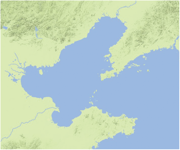
Figure 1: Study area

3.2 FY-4A

There are reflectance differences between ice and water in different spectral channels. The reflectance of seawater and snow decreases with increasing spectral channel wavelength, while the reflectance curve of ice has a single-peaked shape. In the visible light band, the reflectivity of snow is as high as 80%, while the reflectivity of seawater in this band is about 10% or less, and the reflectivity decreases as the wavelength increases. In the near-infrared wavelengths, the reflectivity of snow and ice is significantly lower than that of their respective visible wavelengths. However, there is still a big difference with the reflectivity of seawater in this band. This feature is convenient for the identification of sea ice, and other substances do not have this unique spectral feature.

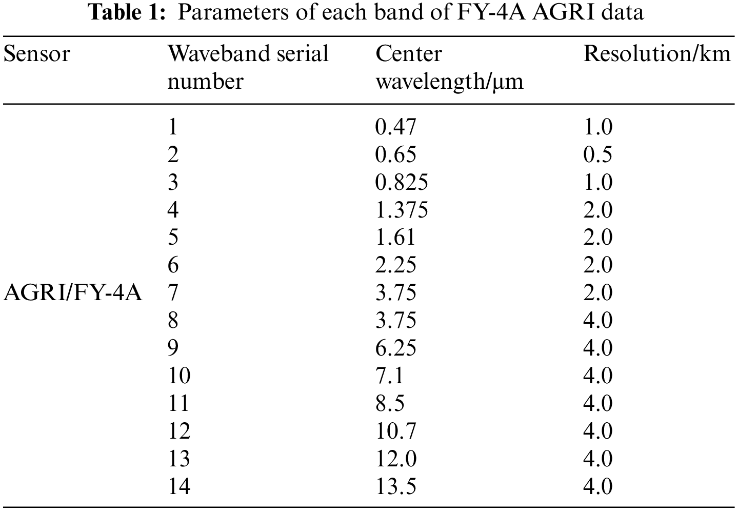
FY-4A was successfully launched on Dec. 11, 2016, and officially received satellite data on May 8, 2018, with the satellite carrying a multi-channel scanning imaging radiometer for rapid area scanning at the minute level. The FY-4A satellite is Chinese second-generation geostationary orbit quantitative remote sensing meteorological satellite. It adopts three-axis stability control technology and can provide important support for weather forecasting and disaster warning in China and the Asia-Pacific region. FY-4A satellite covers visible, short-wave infrared, mid-wave infrared and long-wave infrared wavelengths, with 14 radiation imaging channels, close to the 16 channels of equivalent third-generation satellite products in Europe and the United States [29]. Tab. 1 shows FY-4A. Each band parameter of imaging radiometer data loaded by satellite. Compared with polar-orbiting satellites, FY-4A data has high time resolution. Among them, the average observation data of the full disk is 40 pieces per day, and the average observation data of China is 6 pieces of data per hour, and the average of 165 pieces of data per day. FY-4A data provides data support for the quasi-real-time monitoring of large-scale sea ice in the Bohai Sea.

3.3 Land Removal

The land surface interferes with sea ice identification, and the spectral information of fixed ice areas covered by coastal waters in winter is so close to the land surface snow on shore that it can be easily confused. But land information is basically fixed, and the boundary between land and sea does not move with the seasons. In order to reduce the interference of land on sea ice recognition and retain the information of the Bohai Sea area, the land information needs to be removed first after data preprocessing. The principle of most land removal is to use the reflectivity characteristics of land and sea to distinguish by the waveband threshold method. This method needs to combine the actual situation of the study area to determine the threshold value, and the land and sea-land interface is more complex, and there are more classes of target interferents, leading to some errors in the results, Therefore the key issue is to perform sea-land separation efficiently and accurately, and to remove as much complex land information as possible by precise land removal.

Digital Terrain Model (DTM) digitally describes the ground terrain by various geomorphological factors such as slope, direction, and elevation [30]. Digital Elevation Model (DEM) is one of the subtypes of the digital terrain model, which is a digital simulation of ground terrain using only terrain elevation data, where the value of each grid is an elevation value.

For the problem of land disturbance, this paper uses Digital Elevation Model based land removal. The elevation data are provided by the National Geophysical Center (NGDC) of the United States. ETOPO1 (a topographic data) is a topographic elevation data for the whole world with a spatial resolution of 1 arc minute, which is a solid ground model that represents ground elevation information through a set of ordered arrays, providing basic information about the height of the Earth's surface and related features. Fig. 2 shows the results of land removal based on elevation data, where blue indicates ocean and yellow indicates land.

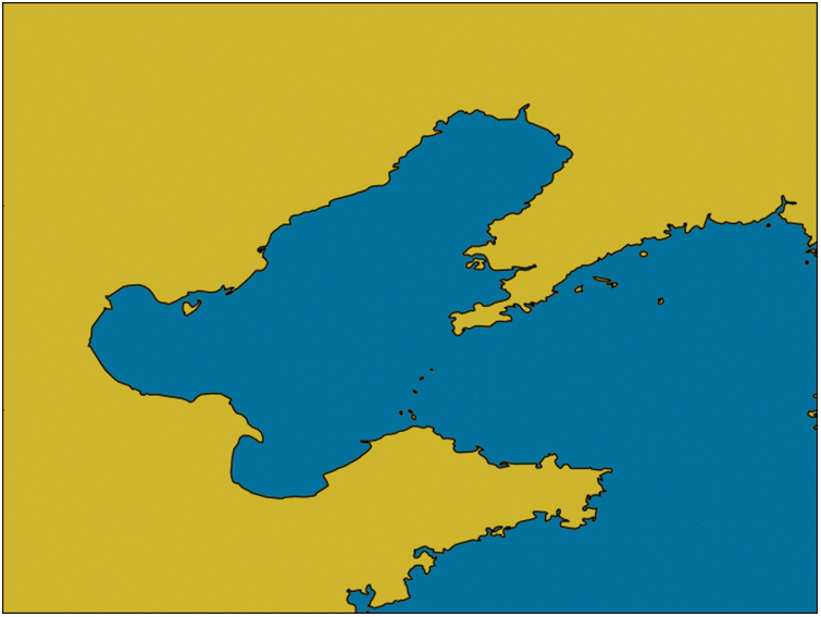
Figure 2: Land removal based on elevation data

3.4 Cloud Detection

Clouds are composed of water droplets and ice crystals in the atmosphere. If they are strongly absorbed in the infrared band, the infrared radiation below the cloud cannot be detected, but the atmospheric radiation above the cloud top can only be detected, resulting in the radiation value observed by the satellite and the actual value, Causes large deviations between the radiation values observed by satellites and the actual values [31]. Cloud detection refers to the estimation of total cloud volume, high cloud volume and cloud top height. The basic principle of cloud detection is to detect the difference in reflectivity and radiance values between clouds and soil, water, ice, snow and vegetation in the visible and infrared bands. Clouds usually have lower brightness temperature values and higher reflectance. In the visible light band, the reflectivity of the underlying surface depends on the difference in the types of ground objects. Among them, the reflectivity of vegetation is the lowest, followed by water, soil and towns have the highest reflectivity, and the reflectivity of clouds is significantly higher than that of the underlying surface, and Changes with height and thickness. In addition, the cloud top temperature is lower in the thermal infrared band, so the brightness temperature of the cloud in the remote sensing image is also lower [32].

In the process of sea ice identification, the Bohai Sea region is severely disturbed by clouds, which poses a great limitation to the use of optical remote sensing data such as FY-4A data. When using FY-4A visible data to identify sea ice in the Bohai Sea, it is easy to misjudge the sea ice due to the presence of clouds, so cloud detection is needed after land removal to effectively eliminate cloud interference.

The cloud detection in this article uses the real-time China cloud detection product of FY-4A satellite data. At present, the cloud detection method of FY-4A uses the standard deviation of the brightness temperature of the 12 μm channel and sets the appropriate characteristic threshold, combined with AGRI’s The visible light channel image then obtains the real-time product of cloud detection [33]. Use cloud detection product data to obtain the result of cloud area recognition, and then generate binary cloud detection data, that is cloud mask.

4  Sea Ice Recognition

4.1 Multichannel Adaptive Thresholding Algorithm for Sea ice Recognition

Since the reflectivity and brightness temperature of ground objects will vary slightly with the seasons, there will be differences in remote sensing data parameters at different times and spaces. In addition, the data coverage in satellite remote sensing images is large, and it is difficult to achieve a good segmentation effect if a fixed threshold is used. In this paper, based on the multi-channel threshold method, an adaptive threshold algorithm is used, which is applied to sea ice identification to improve the sea ice identification results.

Early object detection algorithms based on hand-crafted features mainly rely on the information of objects’ edges and key feature points, and adopt the sliding window operation to determine the location of the object by scanning the whole image [34]. The threshold method is a region-based image segmentation algorithm, and its basic principle is to classify images by setting several threshold intervals. At present, the global empirical threshold segmentation method is widely used in the commonly used sea ice identification methods. During image processing and analysis, the adaptive thresholding algorithm can automatically adjust the processing method, constraints or processing parameters according to the data characteristics of the image target, so that these conditions are adapted to the statistical distribution characteristics and structural features of the image.

OTSU(Japanese scholar OTSU proposed in 1979) method [35] is an adaptive thresholding image segmentation method [36], which is based on the principle of least squares and is suitable for the automatic acquisition of global thresholds in the case of double peaks. The OTSU is used in order to calculate the threshold value to obtain the connected region and then use this threshold to binarize the study region.

In the field of image processing, the most common problem is to extract the target object from the image background. Theoretically, there are two distinct peaks on the image histogram and deep and sharp peaks and valleys between the two peaks, in which case the threshold should be set to the value of the peaks and valleys. In practice, however, the peaks and valleys between the bimodal peaks are not all deep and sharp, but flat and scattered, or the gap between the two peaks is too large, when the value of the peaks and valleys is uncertain. OTSU can solve such problems, specifically, assuming that the grayscale range of the image is [0, L-1], the number of pixels is N, and the number of pixels with gray level i in the image is denoted by ni, then N=n1+n2+…+ni. where the probability of occurrence of a pixel with gray level i is:

Pi=niN,Pi≥0,∑i=0L−1Pi=1(1)

Suppose the pixels in the image are divided into two classes O1 and O2 by thresholding t. O1 and O2 denote the target and background of the image, respectively. Where O1 is the set of all pixels with gray levels in the range of [0, t] and O2 is the set of all pixels with gray levels in the range of [t+1, L-1] [37]. the probabilities of O1 and O2 are:

ω1=∑i=0tPi(2)

ω2=∑i=t+1L−1Pi=1−ω1(3)

The mean values of O1 and O2, respectively, are:

μ1=∑i=0tiPiω1(4)

μ2=∑i=t+1L−1iPiω2(5)

The mean grayscale value of the entire image is:

μ=∑i=0t−1iPi=ω1μ1+ω2μ2(6)

The variances of the two classes are:

σ12=∑i=0t(i−μ1)2Piω1(7)

σ22=∑i=t+1L−1(i−μ2)Piω2(8)

The intra-class variance, inter-class variance and total variance of the two classes in OTSU are:

σW2=ω1σ12+ω2σ22(9)

σB2=ω1(μ1−μ)2+ω2(μ2−μ)2=ω1ω2(μ2−μ1)2(10)

σT2=∑i=0L−1(i−μT)2Pi(11)

The optimal threshold is determined when the variance between classes is maximum, and the formula is as follows:

T=MaxσB2(t)(12)

OTSU algorithms is widely used in many fields, especially in pattern recognition and simulated vision. Some researchers have applied it to medical Magnetic Resonance Imaging, marine oil pollution detection and Computed Tomography image processing [38]. Sea ice recognition is actually to extract sea ice from remote sensing images, but the background in remote sensing images may be more complicated, and there may be no strict double peaks, and it is difficult to determine a reasonable threshold.

4.2 Recognition of Bohai Sea Ice based on Random Forests

Nowadays, when using satellite data information, the meteorological business usually selects only the data under clear sky conditions and eliminates all the fields of view or data polluted by clouds, this processing method is relatively simple, but the elimination of clouds will waste a large amount of satellite observation data. In practice, the proportion of the basic cloud-free situation in the Bohai Sea region is relatively small. In particular, MODIS data such as data acquisition frequency of 1–2 days is likely to result in the rejection of dozens of days in a year, and the waste of data appears more serious.

The multi-channel dynamic threshold method for sea ice identification, which cannot achieve sea ice identification under cloud coverage, and the Bohai Sea region also appears to be fully covered by clouds, and there is continuous cloud cover over Liaodong Bay in winter, and this situation cannot achieve detection of sea ice. In fact, sea ice recognition is also the classification of sea ice and other interference objects. The classification method can be used to train and model the input data and classify the sea ice classification results.

The random forests algorithm uses decision trees as the base learner for integrated learning, where the decision tree is a tree-like data structure composed of root nodes, intermediate nodes and leaf nodes. The process of the algorithm is to first use the Bagging algorithm to randomly draw data samples from the sample training set D to obtain k independent training sample sets {D1,D2,…,Dk} and then construct the corresponding decision trees according to the different training sample sets. k sample sets are generated k decision trees {F1,F2,…,Fk}. The criterion for selecting node features for the decision tree is the Gini coefficient, and if there are N category instances in the training set D, the Gini coefficient is calculated as follows:

Gini(D)=1−∑i=1k[P(i)∗P(i)](13)

where, P (I) represents the proportion of class I sample data in the data set on the current node. When the training sample set D is divided into two subsets D1 and D2 by using the characteristic attribute F, the definition formula of Gini coefficient is:

Gini=Gini(D)−Gini(D1)−Gini(D2)(14)

For each CART (classification and regression tree) decision tree, the training sample subset is started from the root node for training. If the training reaches the termination condition of splitting, the current node is set as a leaf node. If the termination condition of the split is not reached, then use the Gini coefficient to select an optimal feature from the N-dimensional features, and then divide the sample data on the current node into the left and right child nodes, and then continue to train other untrained nodes. Until all nodes are trained or are marked as leaf nodes. After training all CART, each tree can predict the test sample data set according to the node threshold, and use the voting method to determine the final classification result of the entire random forests based on the classification results of each tree. The features generated by using the decision tree alone usually have the problem of overfitting. Random forests first calculate the importance of features and then performs feature selection. The goal of random forests features selection is to select a small number of features that can meet the requirements of use, preventing overfitting. The sea ice in the Bohai Sea changes with the seasons, and some spectral channels of FY4A are also affected by solar radiation, so the use of random forests for feature selection is more suitable for practical application scenarios. There are many new algorithms proposed based on random forests such as XGboost (A machine learning method) [39]. The time complexity and space complexity of XGboost is much higher than that of random forests. XGboost needs to store not only the feature values but also the index values of the gradient statistics of the samples corresponding to the features. Therefore, random forests deployment on lightweight servers has better efficiency. In practical application scenarios, the Bohai Sea ice recognition algorithm usually runs on portable devices during field operations, and cannot run models with high complexity.

This article is based on FY-4A data and 6132 pixels in the Bohai Sea to classify the Bohai Sea ice. For FY-4A data and multi-channel adaptive thresholding method of Bohai Sea ice identification the binary data of Bohai Sea Ice identification results of the adjacent 24-hour multi-channel adaptive thresholding method are used as input and labeled as the sea ice operational data of the 24th hour.

5  Experiment and Result

5.1 Evaluation Method

The FY4A geostationary meteorological satellite started work in 2018 and began to provide stable quality product data in 2019. In this paper, we use all available data for three years from 2019 to 2021, and divide the data into 3 folds by year. To prevent the occurrence of over-fitting and under-fitting problems of the model and evaluate the generalization ability of the model, the model training in this paper adopts the 3-fold cross-validation method.

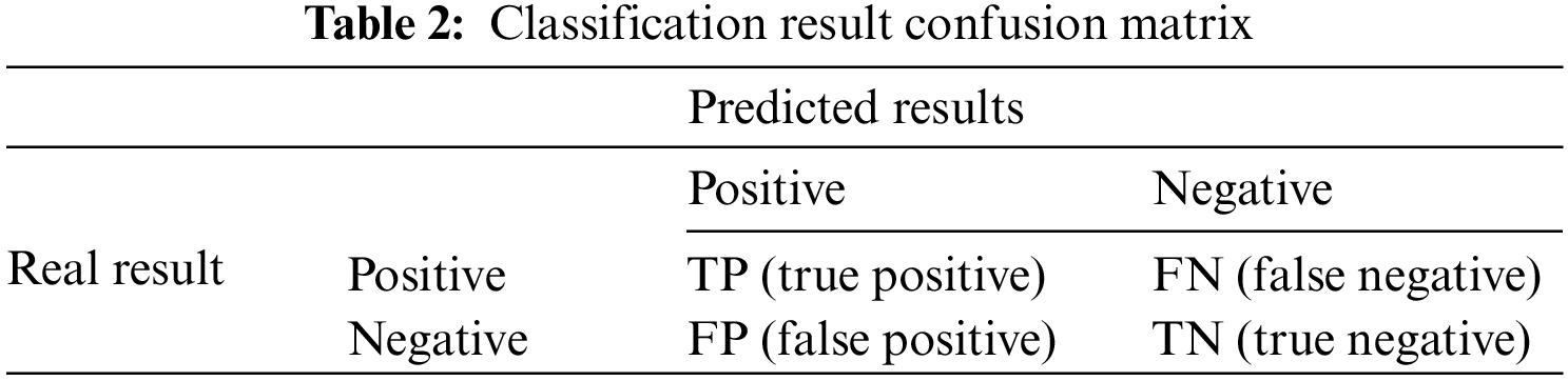
In the experiments of this chapter, multiple evaluation criteria are used to evaluate the random forests sea ice classification model. In this paper, a binary confusion matrix is used as shown in Tab. 2. The confusion matrix can clearly see the sample classification and is used to calculate the evaluation index of the classification.

Accuracy rate: The ratio of the number of samples with correct prediction results to the total number of samples, the calculation formula is:

Accuracy=TP+TNTP+TN+FP+FN(15)

Precision rate: Among all the samples predicted to be sea ice, the ratio of sea ice samples that are predicted to be correct samples is calculated as:

Precision=TPTP+FP(16)

Recall rate: The ratio of samples that are correctly predicted to be sea ice to all samples that are actually sea ice is calculated as:

Recall=TPTP+FN(17)

F1-score: It is related to the precision rate and recall rate, which can better express the classification effect of the model. The calculation formula is:

F1−score=2∗Precision∗RecallPrecision+Recall(18)

5.2 Multichannel Adaptive Threshold Algorithm

The results of applying the OTSU dynamic thresholding algorithm for sea ice identification are shown in Fig. 3, and two days of experimental data on January 3, 2020 and February 12, 2020 are selected for demonstration, where yellow indicates land, blue indicates ocean, and white indicates sea ice. Figures (a) and (d) in Fig. 3 represent the sea ice identification results based on the Multichannel adaptive threshold method, figures (b) and (e) represent the albedo-bright temperature threshold method identification results, and figures (c) and (f) represent the sea ice business. As can be seen from the figure, the Multichannel adaptive thresholding algorithm for sea ice identification in the Bohai Sea greatly improves the sea ice identification results compared with the albedo -bright temperature thresholding method. The Multichannel adaptive thresholding method is more suitable for Bohai Sea ice identification under clear sky conditions, and the dynamic threshold selection by dynamic threshold algorithm can reduce the workload of manual threshold adjustment and selection caused by seasonal change variation, which also shows that FY-4A data can be applied to Bohai Sea ice identification.

Our process for identifying sea ice in the Bohai Sea using adaptive thresholding is as follows:

1): Input the data from channel 2, 3, 5, 12 and 13, and calculate IST (Ice Surface Temperature) and NDSI (Normalized Difference Snow Index);

2): Normalize channel 2, IST and NDSI data to the 0–100 range

3): Interval alienation of channel 2, IST and NDSI data

4): Interval quantification of channel 2, IST and NDSI data

5): Set high and low thresholds for reflectance, IST, and NDSI, and use the thresholds for recognition, respectively. If the two recognition results are consistent, end; if not, proceed to the next step;

6): Determine dynamic thresholds. For the pixels with inconsistent recognition results, all the inter-class variances are calculated in sequence according to OTSU, and finally the inter-class variances are compared to determine a new threshold.

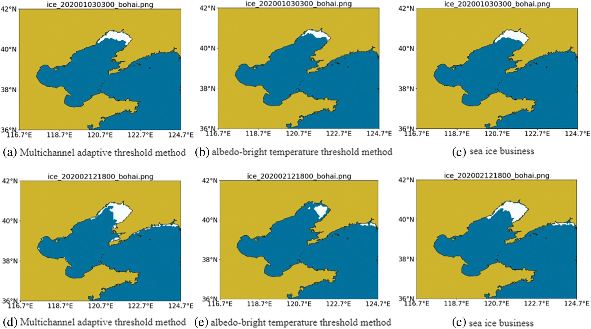
Figure 3: Comparison of recognition results

5.3 Random Forests

This paper is based on the random forests classification model to train and verify the Bohai Sea ice recognition model. The performance of the random forests classification model is mainly affected by the number of decision trees and the maximum depth of the trees, so this paper focuses on these two parameters for the study of tuning the parameters. A larger number of policy trees can lead to a better and more stable performance of the model, but it also makes the training slower. The tuning process uses a cross-validation method for training and validation, and the average score of cross-validation is used as the evaluation criterion. The learning curve is used to find the optimal value to correct the classification accuracy to a higher level. The number of decision trees and the maximum depth of the model inputs are parametrized separately, with the number of decision trees tested at 10 intervals from 1 to 400 and the maximum depth tested at 1 interval from 1 to 50 to determine the optimal parameter configuration for both input models. The workflow chart of the algorithm in this paper is shown in Fig. 4

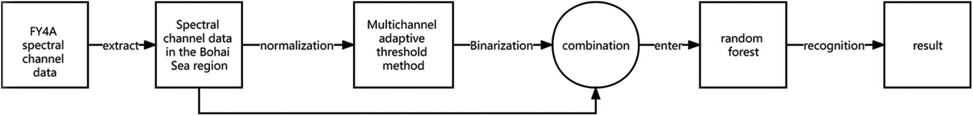
Figure 4: Workflow chart

Firstly, the model input is tuned to the sea ice identification results, and the learning curve of the specific tuning process is shown in the following Figs. 5 and 6. The number of decision trees was tested at intervals of 10 from 1 to 400, starting with an approximate range of 50 to 70, where the best number of decision trees was derived as 61 with a maximum score of 0.91992762. After further adjusting the parameters within this range, it is concluded that the number of optimal decision trees is 55, and the maximum score is 0.92009075. The model score has been improved. The maximum depth of the tree was tested at intervals from 1 to 50, and the optimal depth of the model was experimentally determined to be 5.

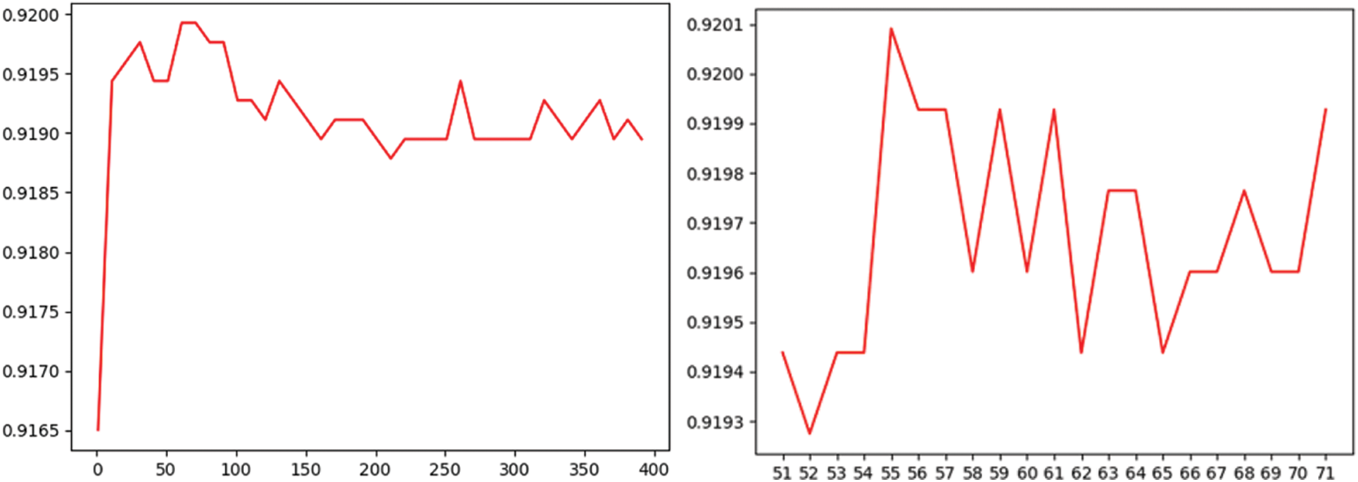
Figure 5: Quantity learning curve of decision tree

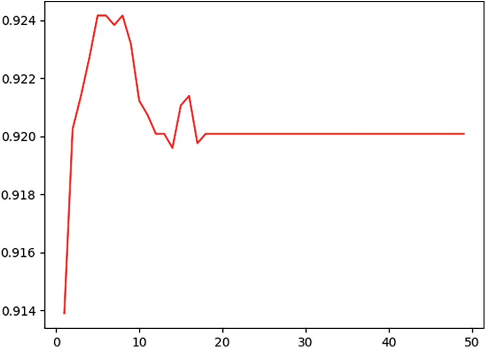
Figure 6: Decision tree maximum depth learning curve

5.4 Experimental Results

The experimental results were compared and analyzed with the results of sea ice operational data. Accuracy rate, Precision rate, Recall rate and F1-score were calculated by TP, FP, TN and FN. The sea ice in the Bohai Sea only exists in winter. We trained the model on the balanced and imbalanced datasets, respectively. The results show that the problem of imbalanced data can be overcome by using the random forests method. The experimental results are selected from the experimental data on December 25, 2020, as shown in the following Tabs. 3, 4 and Fig. 7

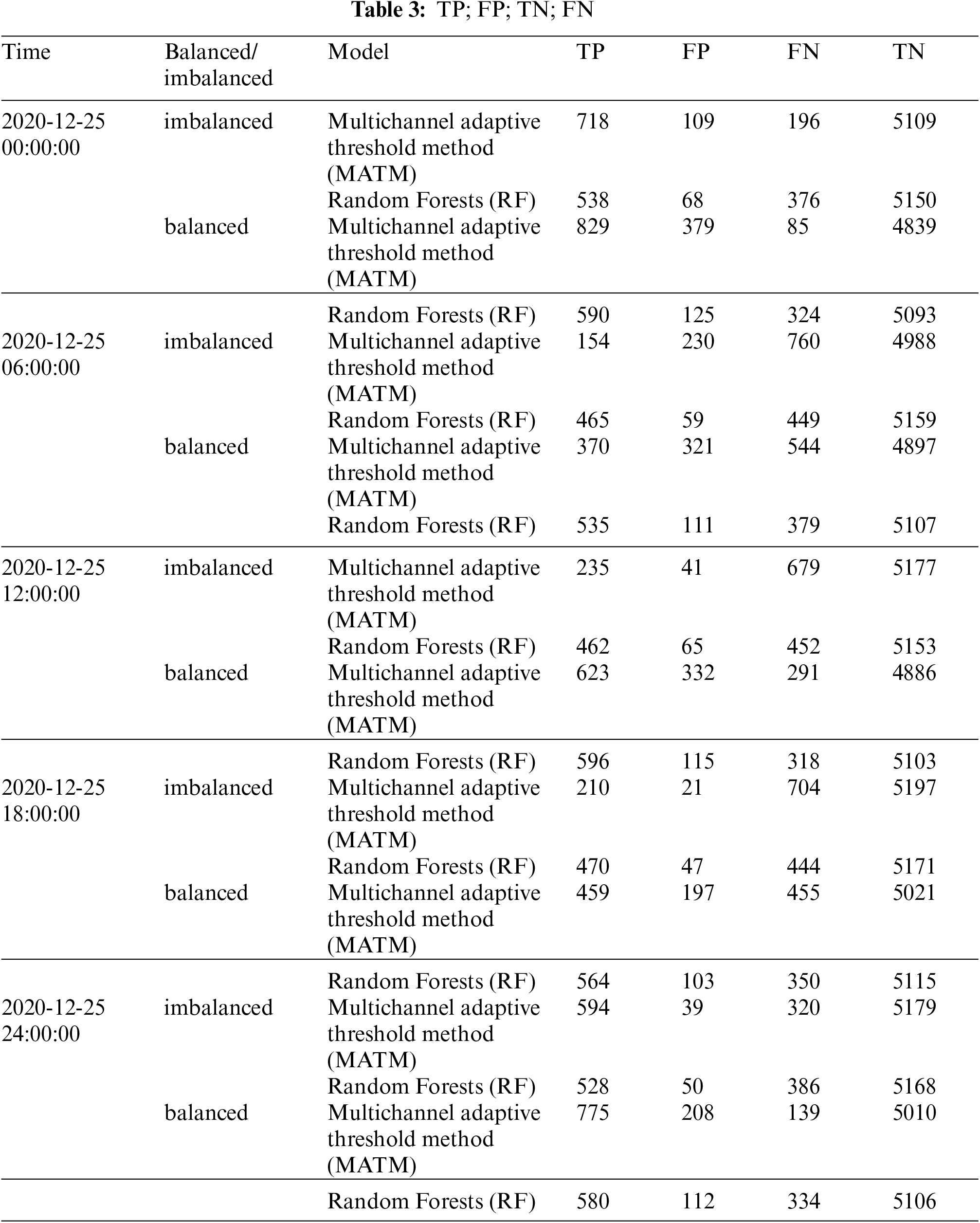
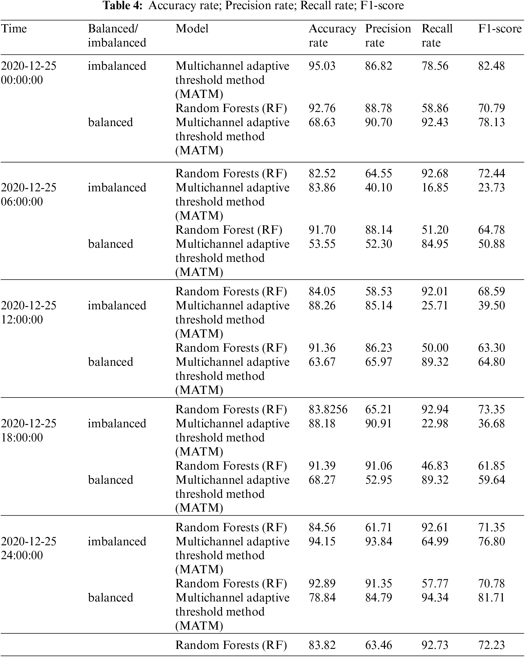
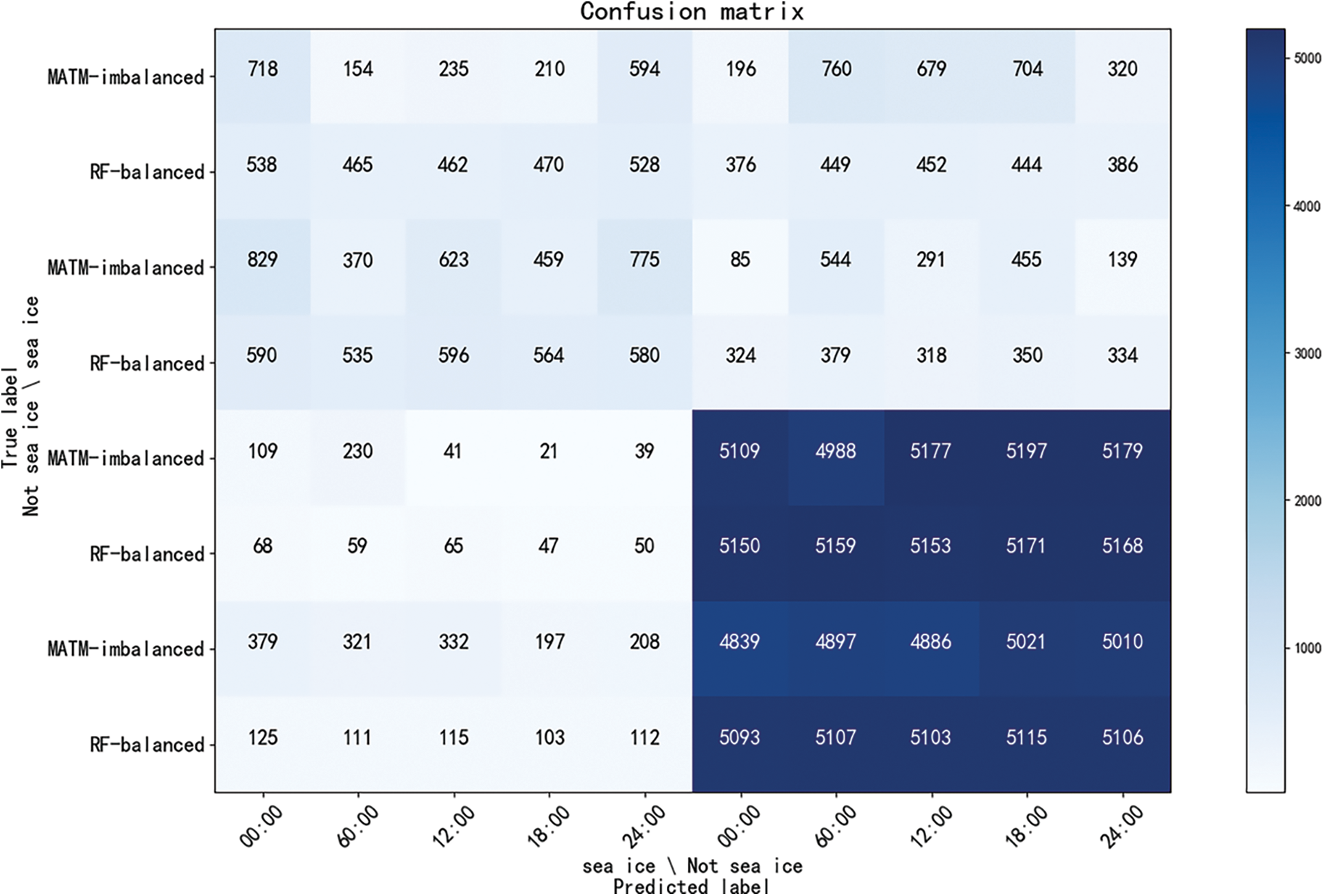
Figure 7: Confusion matrix

Comparing the two models, we can find that the random forests model has better classification results and smoother performance. The result plots are shown below, and (a), (b), (c) and (d) in Fig. 8 show the Multichannel adaptive threshold method results, random forests identification results, MODIS sea ice product results and sea ice business results, respectively. From the figure, it can be seen that: under non-clear sky conditions, the sea ice identification results using the Multichannel adaptive threshold method are very poor due to cloud coverage, especially in the Liaodong Bay waters, Bohai Bay and Laizhou Bay region. Compared with the results of the Multichannel adaptive threshold method and MODIS sea ice products, the random forests classification algorithm has improved, and is closer to the sea ice business results.

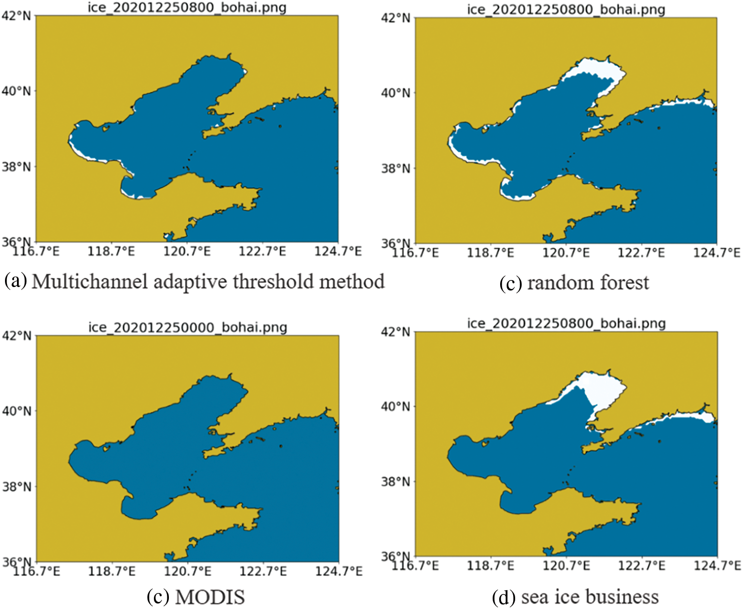
Figure 8: Comparison of recognition results

The random forests algorithm is close to the results of the sea ice business, and the recognition effect is better than that of the Multichannel adaptive threshold method; Compared with MODIS sea ice products, random forests greatly improve the effect of sea ice recognition. Therefore, through the analysis of the experimental results, the random forests algorithm is more suitable for the recognition of sea ice in the Bohai Sea. Feature extraction by random forests algorithm can reduce the workload of threshold adjustment caused by seasonal changes. It also shows that FY-4A data can be applied to sea ice recognition in the Bohai Sea. Due to the lack of satellite remote sensing data, when there is a large area of cloud coverage above the Bohai Sea, the effect of sea ice recognition by the Multichannel adaptive threshold method decreases significantly, and even the sea ice cannot be recognized. Because of this situation, using random forests can reduce the influence of clouds on sea ice identification.

6  Conclusion

In this paper, the existing sea ice identification algorithms are studied and found to be basically for sea ice identification under clear sky conditions without considering the identification under cloud cover. Therefore, this paper combines the results of sea ice identification by the threshold method and designs and implements a random forests based sea ice classification algorithm for the Bohai Sea to achieve more effective sea ice identification results under clouds. The detection and removal of clouds in sea ice identification algorithm is crucial to sea ice identification and determines the accuracy of identification results. After the experiment, it can be seen that the data of FY-4A cloud detection product has some errors in the detection results of clouds, and the subsequent work can further research on the detection of clouds and improve the effect of sea ice identification. Geostationary weather satellites work on the same principle and have similar observation channels, so theoretically the random forests method can be used for most geostationary weather satellites. There are many traditional meteorological methods to achieve sea ice identification, and in the future, we intend to try new methods such as deep learning methods to identify sea ice to improve sea ice identification.

Funding Statement: This research was supported by the National Natural Science Foundation of China under Grant No.61772280 and No.62072249

Conflicts of Interest: The authors declare that they have no conflicts of interest to report regarding the present study.

This work is licensed under a Creative Commons Attribution 4.0 International License, which permits unrestricted use, distribution, and reproduction in any medium, provided the original work is properly cited.