Computers, Materials & Continua DOI:10.32604/cmc.2022.030372
Article

Reversible Data Hiding in Encrypted Images Based on Adaptive Prediction and Labeling

Jiaohua Qin1,*, Zhibin He1, Xuyu Xiang1 and Neal N. Xiong2

1College of Computer Science and Information Technology, Central South University of Forestry & Technology, Changsha, 410004, China
2Department of Mathematics and Computer Science, Northeastern State University, Tahlequah, 74464, OK, USA
*Corresponding Author: Jiaohua Qin. Email: qinjiaohua@163.com
Received: 24 March 2022; Accepted: 07 May 2022

Abstract: Recently, reversible data hiding in encrypted images (RDHEI) based on pixel prediction has been a hot topic. However, existing schemes still employ a pixel predictor that ignores pixel changes in the diagonal direction during prediction, and the pixel labeling scheme is inflexible. To solve these problems, this paper proposes reversible data hiding in encrypted images based on adaptive prediction and labeling. First, we design an adaptive gradient prediction (AGP), which uses eight adjacent pixels and combines four scanning methods (i.e., horizontal, vertical, diagonal, and diagonal) for prediction. AGP can adaptively adjust the weight of the linear prediction model according to the weight of the edge attribute of the pixel, which improves the prediction ability of the predictor for complex images. At the same time, we adopt an adaptive huffman coding labeling scheme, which can adaptively generate huffman codes for labeling according to different images, effectively improving the scheme’s embedding performance on the dataset. The experimental results show that the algorithm has a higher embedding rate. The embedding rate on the test image Jetplane is 4.2102 bpp, and the average embedding rate on the image dataset Bossbase is 3.8625 bpp.

Keywords: Reversible data hiding; adaptive gradient prediction; huffman coding; embedding capacity

1  Introduction

With the continuous development of digital media technology [1], the security problem of information transmission is also becoming more and more serious. Information hiding plays a vital role in information security as an essential information protection technology. Information hiding refers to the stealthy embedding of information into a carrier without arousing suspicions [2], such as steganography [3,4] and digital watermarking [5,6]. However, these methods will make certain changes to the carrier, resulting in the receiver being unable to recover the original carrier after extracting the secret information, which is terrible in the military and medical fields because the carrier’s original information is also terrible essential. reversible data hiding (RDH) can effectively solve this dilemma and therefore has become a popular research direction, which can extract secret information accurately and recover the original image without image quality degradation. Early proposed RDH techniques are mainly implemented in the plaintext domain and can be classified into three categories depending on the embedding ways: difference expansion [7,8], histogram shifting [9,10], and lossless compression [11,12]. However, with the increasingly severe privacy leakage problem, coverless steganography [13], information hiding technology in the ciphertext domain, and multimodality [14] have attracted more and more attention.

Therefore, based on RDH, researchers have proposed reversible data hiding in encrypted images (RDHEI), which additionally allows the data hider to hide additional information in the ciphertext. As shown in Fig. 1, the existing RDHEI technologies are mainly based on RDH combined with two mechanisms: vacating room after encryption (VRAE) [15–18] and reserving room before encryption (RRBE) [19–25]. VRAE can hide data by the redundant space after image encryption, for example, Zhang et al. [16] proposed an RDHEI scheme based on image block embedding in 2011, embedding data by modifying a part of encrypted data and supporting the receiver to extract data and recover the image in a separable manner, but the image block size limits its capacity; Zhang et al. [17] reserved more space for auxiliary information and secret data by compressing the least significant bit (LSB) of encrypted pixels; Hong et al. [18] proposed a new smoothness evaluation function to evaluate the fluctuation of pixels, which effectively improves the low embedding rate in the case of small image blocks. As seen, VRAE cannot achieve good embedding performance as the encryption operation inevitably destroys the spatial correlation of the original image. On the contrary, RRBE makes full use of the redundant information of image pixels to reserve space before image encryption and then transfers it to the encrypted image with higher embedding capacity. Obviously, it makes more sense for us to adopt RRBE as the research subject.

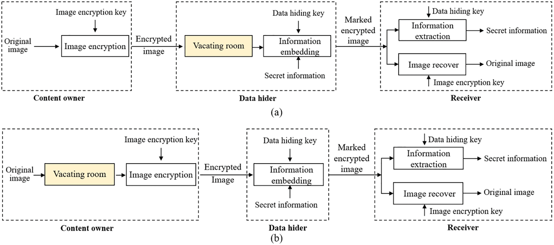
Figure 1: Two frameworks of RDHEI algorithm: (a) VRAE (b) RRBE

Yi et al. [22] proposed an RDHEI scheme based on parametric binary tree labeling (PBTL), which proposed a PBTL pixel labeling scheme to ensure that the scheme can extract data and restore images reversibly. Wu et al. [23] proposed an RDHEI scheme based on improved parametric binary tree labeling (IPBTL), which improves upon scheme [22]. The IPBTL classifies and labels pixels according to the prediction error of the image, leaving space for data embedding and improving the embedding rate of the scheme. However, its predictor and coding efficiency still affect the embedding performance. Yin et al. [24] designed an RDHEI method based on multiple most significant bit prediction and huffman coding (MMPHC), which compared the most significant bit (MSB) of the original pixel with the predicted pixel, used the bits of the same sequence as a label, and marked the pixel with a pre-defined huffman code. However, experiments show that predefined huffman encodings do not perform markup well. To take advantage of the correlation of adjacent pixels, Yin et al. [25] proposed an RDHEI scheme based on pixel prediction and bit-plane compression (PPBC) by utilizing the correlation of neighboring pixels, which reserved more space for data embedding due to its better compression effect. Despite the exemplary achievements of all the above-mentioned methods, they share a common drawback: the used classifier median edge detector (MED) has a small receptive field, its prediction form is too homogeneous to predict complex images. Besides, the existing codes still have many shortcomings as an essential aspect. Most of the methods use the correlation between pixels to generate the embedding space and achieve the reversible embedding and extraction of secret information by establishing the mapping relationship between the prediction error of the pixel and the marking code. While this coding approach has two drawbacks: 1. The sequence of labeling depends on the set predefined parameters, and different parameter settings may yield different embedding rates, which leads to instability of embedding rates. 2. It uses a uniform sequence for labeling different types of images, so it has some limitations, e.g., it does not work well on large image datasets.

To solve the above problem, we design an adaptive gradient predictor (AGP) and use an adaptive huffman coding labeling method to propose a new RDHEI algorithm. The proposed adaptive gradient predictor uses eight adjacent pixels that combine four scanning methods (i.e., horizontal, vertical, diagonal, and anti-diagonal) in prediction, whose weights can be adaptively adjusted to construct a local linear prediction model based on the edge properties of the neighboring pixels. The adaptive huffman coding tagging algorithm statistically analyzes the prediction errors of different images and then adaptively generates the corresponding coding rules to achieve better results on multiple datasets.

The main contributions of this paper are as follows:

1.    We propose a new and well-performing adaptive gradient prediction model, which can assign different weights to the surrounding pixels according to the neighborhood complexity of the target pixels in the prediction process, and consider the impact of pixel changes in different directions on the prediction, which better characterizes the local features of the target pixels.

2.    We further combine the proposed AGP with the adaptive huffman coding labeling method to statistically analyze the prediction errors of different images and adaptively generate different huffman codes for labeling.

3.    Experimental results show that our scheme achieves higher embedding rates, especially on large datasets, e.g., the average embedding rate of the BOSSbase dataset reaches 3.8625 bpp, which exceeds other state-of-the-art algorithms.

The rest of this paper are organized as follows. Section 2 presents the proposed scheme proposed, Section 3 presents the experimental evaluations, and Section 4 concludes the article.

2  Proposed Scheme

This section illustrates reversible data hiding in encrypted images based on adaptive gradient prediction and code labeling method. The algorithm framework is shown in Fig. 2, which can be divided into three parts. In the first part, the content owner first predicts and encrypts the original image using AGP and image encryption keys. Then, the huffman coding is adaptively generated according to the prediction error, and the coding rules are embedded into the encrypted image. In the second part, after obtaining the marked encrypted image, the data hider first extracts the encoding rules to determine the position of the reserved room. Then the encrypted information is embedded in the reserved room to form a marked stego image. In the third part, the receiver can perform three operations. The original secret information can be extracted when the information hiding key is obtained. The original image can be recovered when the image encryption key is obtained. The original image and the secret information can be obtained simultaneously when both keys are received.

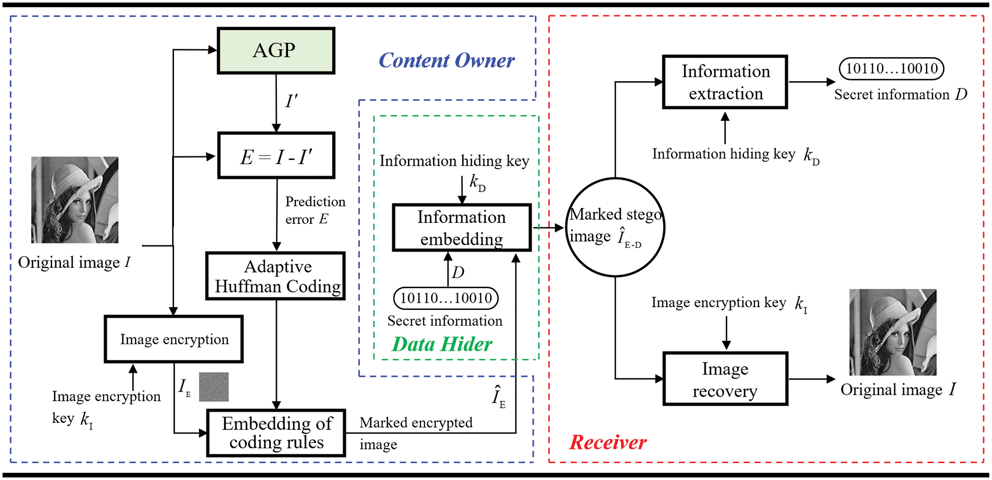
Figure 2: The framework of the proposed scheme

2.1 Image Preprocessing

Before embedding the information, the content owner preprocesses the original image to reserve room for the embedded information. The preprocessing process of our scheme mainly includes two parts. First, the prediction error is calculated according to the AGP, and then the prediction error is statistically analyzed, and the huffman code is adaptively generated.

2.1.1 Adaptive Gradient Prediction

The proposed adaptive gradient predictor AGP is shown in Fig. 3, which can meet the multi-directional requirements of natural images for texture attributes by perceiving pixel changes from four directions: horizontal, vertical, diagonal, and anti-angle around the target pixel. Its weight distribution of different gradient pixels is adjusted according to the position of the target pixel. The specific prediction steps can be divided into two stages. The gradient strength of the predicted pixel is calculated first. Then, according to the gradient environment where the target pixels are located, the weights are adaptively adjusted to construct a local linear prediction model for prediction. The pixels in the first row and the first column remain unchanged as reference pixels during the image prediction process.

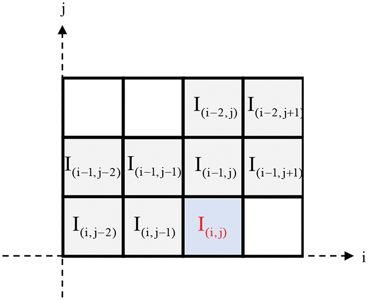
Figure 3: Predictive template used by AGP

Before calculating the local complexity, the gradient strength of the local pixel is estimated by Eq. (1).

Gh=∑t=01|I(i−1,j+1-t)−I(i−1,j−t)|+∑t=01|I(i−t,j−1)−I(i−t,j−2)|Gv=∑t=01|I(i−2,j+1-t)−I(i−1,j+1-t)|+∑t=01|I(i−1,j−1−t)−I(i,j−1−t)|Gd=|I(i−1,j−2)−I(i,j−1)|+|I(i−2,j)−I(i−1,j+1)|Ga=|I(i−1,j−1)−I(i,j−2)|+|I(i−2,j+1)−I(i−1,j)|(1)

where Gh, Gv, Gd, and Ga represent the gradient strengths of the predicted pixels from the horizontal, vertical, diagonal, and anti-diagonal directions, respectively.

The predicted value of the pixel in our scheme is obtained according to the weighting of the domain pixels. According to the texture properties of the pixels, the prediction cases are divided into sharp edges and non-sharp edges. Sharp edges indicate significant changes in surrounding pixels, and non-sharp edges indicate regular or minor changes in surrounding pixels. When the pixel is at a sharp edge, the weight distribution of the scanning mode is shown in Fig. 4.

As shown in Fig. 4, to adapt the scheme to images with complex textures, this scheme adjusts the scanning mode’s weight according to the neighborhood complexity of pixels. When the target pixel is on a sharp horizontal edge, its predicted value is mainly affected by the pixels in the horizontal direction, so the weight of the horizontal scanning method is larger. The weight of the diagonal direction is also divided into strong edges and weak edges, which are determined according to the surrounding gradient strength. When the pixel is on a sharp edge, the predicted value is obtained by

I′(i,j)=⌊ γt+ωΔt ⌋,t={ 0Gv−Gh>T11Gh−Gv≥T1ω={ 1| Gd−Ga |>T212| Gd−Ga |≤T2Δ0=132(2(I(i-1,j-1)−I(i-1,j-2))+(I(i-1,j-2)−I(i,j-1))+(I(i-1,j+1)−I(i-2,j)))Δ1=132(2(I(i-1,j+1)−I(i-2,j+1))+(I(i-2,j+1)−I(i-1,j))+(I(i-1,j-1)−I(i,j-2)))γ0=I(i,j-1)+I(i,j-1)−I(i,j-2)2,γ1=I(i-1,j)+I(i-1,j)−I(i-2,j)2(2)

where γ0, γ1 represent the dominant values when predicting pixels at sharp horizontal and vertical edge locations. Δ0, Δ1 represent the influence of pixels in the diagonal and anti-diagonal directions on the predicted value during prediction, respectively. t is used to judge that the predicted value is mainly affected by the pixels in the vertical or horizontal direction. ω represents the weight of the scanning mode of different gradient strengths.

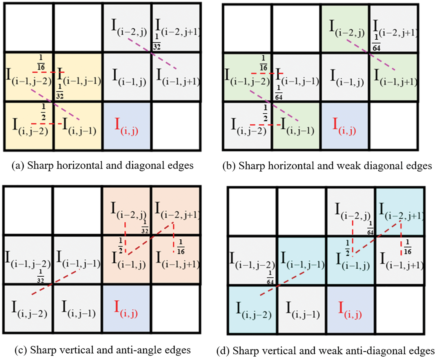
Figure 4: Weight assignment of scan mode for sharp edges

When the pixels are on sharp horizontal and diagonal edges, the vertical and diagonal pixels vary greatly. The predicted pixels are mainly affected by the horizontal and nearest diagonal pixels. When the pixels are on sharp vertical and diagonal edges, the horizontal and diagonal pixels vary greatly. The predicted pixels are mainly affected by the vertical and nearest diagonal pixels. When the pixels are on a non-sharp edge since the pixels from all directions do not change much, a prediction operator θ is calculated by Eq. (3). Then the prediction value is fine-tuned according to the prediction operator and the pixel’s position.

Non-sharp edges are divided into ordinary edges and weak edges according to the gradient strength around the pixel. When the pixels are on a non-sharp edge, the weight distribution of the scanning mode is shown in Fig. 5.

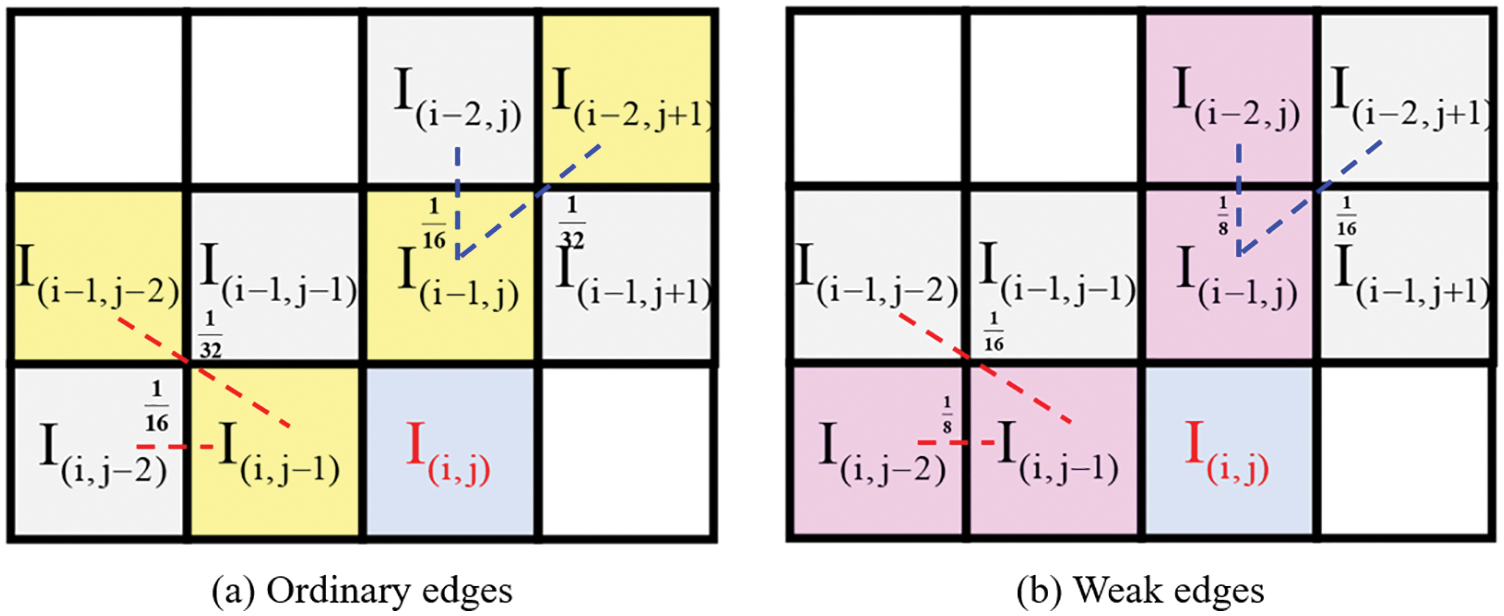
Figure 5: Weight assignment of scan mode for ordinary edges and weak edges

where the red and blue lines in Fig. 5 represent the pixels participating in the prediction when the pixels are on non-sharp horizontal and vertical edges, respectively. Pixel predictions on non-sharp edges are calculated by Eq. (4).

θ=⌊I(i−1,j+1)2+2I(i−1,j)−I(i−2,j)8+2I(i,j−1)−I(i,j−2)8⌋(3)

I′(i,j)={ εt,(| Gv−Gh |>T4)εt+θ2,(| Gv−Gh |<T4),t={ 0Gv−Gh>T31Gh−Gv>T3ε0=θ+I(i,j-1)2+I(i,j-1)−I(i,j-2)8+I(i,j-1)−I(i−1,j-2)16ε1=θ+I(i-1,j)2+I(i-1,j)−I(i-2,j)8+I(i-1,j)−I(i-2,j+1)16(4)

where ε0, ε1 represent the dominant values when predicting pixels at non-sharp horizontal and vertical edge locations. t is used to judge that the predicted value is mainly affected by the pixels in the vertical or horizontal direction.

The above prediction coefficients and thresholds are selected according to an exhaustive algorithm. A threshold selection experiment is set up in Section 3.1, which verifies that our scheme can achieve the best embedding rate under the selected threshold. After calculating the predicted value of the pixel, the prediction error of the pixel can be calculated by Eq. (5).

E(i,j)=I(i,j)−I(i,j)′(5)

2.1.2 Generation of Adaptive Huffman Codes

Our scheme adopts an adaptive huffman coding [26] for pixel marking to ensure that the scheme achieves a better coding effect. For different pictures, the scheme first performs statistical analysis on the prediction error and then adaptively generates huffman coding according to the probability of the error occurrence. The following will introduce the adaptive huffman coding marking process in detail with an example.

First, count the frequency of prediction errors. Since the length of the huffman code used for marking is no longer than 8 bits, the average frequency of each codeword is 1/256. This feature can be used as a threshold for dividing the frequency of prediction errors. Pixels with prediction error frequency within the average frequency range are classified as embeddable pixels, and those not within the range are non-embeddable pixels. Therefore, the scheme divides the remaining pixels except for the reference pixels into two parts: embeddable pixels and non-embeddable pixels. Taking the 6×6 block of the Lena image as an example, the adaptive huffman coding generation process shown in Fig. 6 is performed.

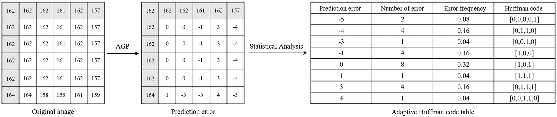
Figure 6: Adaptive huffman coding generation

The blocks selected in Fig. 6 do not contain non-embeddable pixels for the convenience of representation. The scheme uses the same code for marking for non-embeddable pixels whose error frequency is less than 1/256.

2.1.3 Image Encryption

After obtaining the prediction error of the original image I and huffman encoding, the original image is encrypted using a stream cipher. First, a pseudo-random matrix P of size m×n is generated using the key. Then, convert I and P into binary form and encrypt them by bitwise XOR:

IEk(i,j)=Ik(i,j)⊕Pk(i,j) k=1,2,⋯,8(6)

where 1≤i≤m, 1≤j≤n. IEk(i,j), Ik(i,j), and Pk(i,j) represent an encrypted image IE, original image I, and the kth bit of the (i,j)th pixel in the error matrix P, respectively.

2.1.4 Labeling with Adaptive Huffman Codes

After adaptively generating the huffman code, the pixels can be labeled. All pixels are divided into reference pixels, embeddable pixels, and non-embeddable pixels. The reference pixel is not labeled, and its room is used to embed the huffman coding rule, that is, Correspondence between prediction error and huffman code. The original value of the reference pixel is stored in the reserved room as part of the auxiliary information. The bits of the non-embeddable pixels replaced by the huffman code are also stored as auxiliary information. The remaining room of the embeddable pixels is used to embed auxiliary information and secret information. Taking the 4×4 block of the Lena image as an example, the pixel labeling process is as shown in Fig. 7.

To prevent the generated huffman code from being the same as the original bit of the labeled part of the pixel, resulting in the leakage of image information. As shown in Fig. 7c, the scheme adopts sorting in reverse order. This method ensures that the resulting marked encrypted image has a higher level of security. The part marked in red in Fig. 7d represents the labeled bit, and ‘-’ represents the reserved room for data embedding.

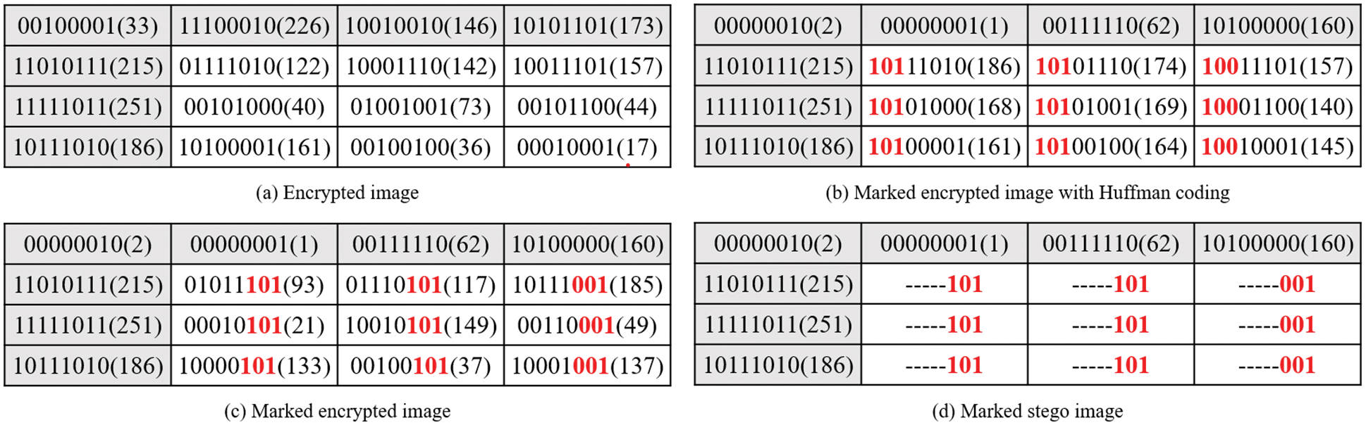
Figure 7: Pixel labeling process

2.2 Information Embedding

Before data hiding, the huffman coding rules are extracted from the reference pixels of I^E, and then the position of the reserved room is determined. To ensure the security of the embedded information, the secret information needs to be encrypted by the information hiding key kD before embedding. Finally, the information is embedded in the reserved room by bit replacement.

2.3 Information Extraction and Image Recovery

After receiving the marked stego image, the receiver implements different operations according to the key type obtained.

2.3.1 Information Extraction

The receiver who obtains the data hiding key kD can extract the data: the receiver first extracts the coding rules from the reference pixels of I^E−D and determines the position of the reserved room. Then, the embedded secret data and auxiliary information are extracted. The encrypted data can be decrypted to recover the original secret information according to the key kD. Fig. 8 shows the process of extracting secret information.

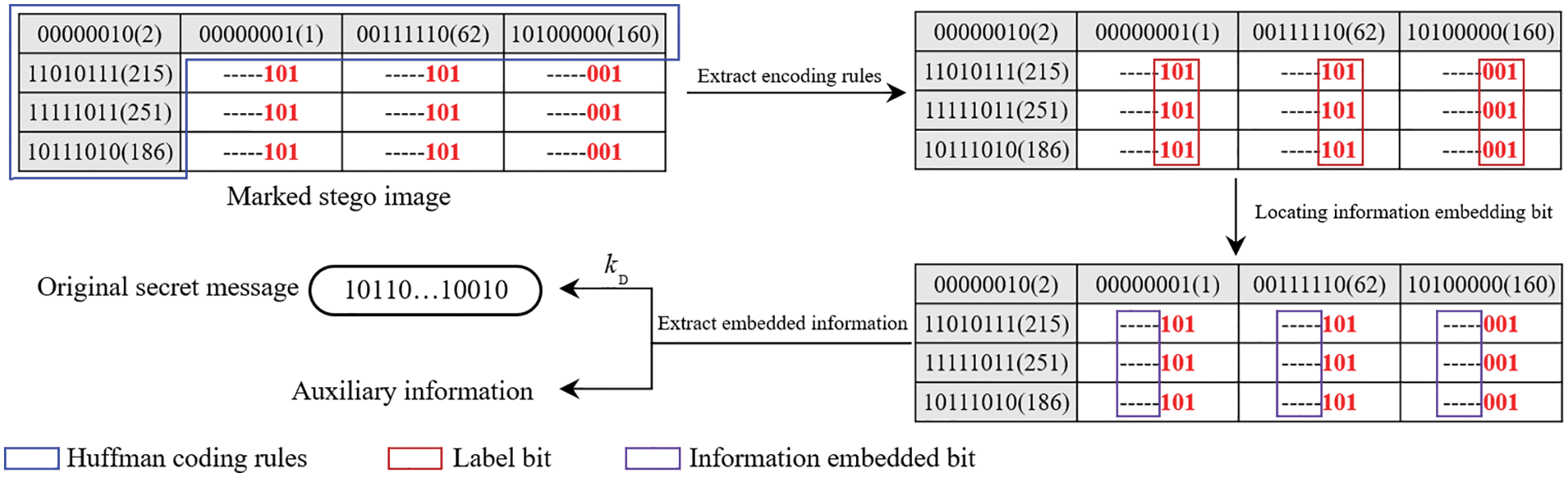
Figure 8: The process of extracting secret information

2.3.2 Image Recovery

The receiver who obtains the image encryption key kI can recover the original image: after extracting the auxiliary information, the encrypted reference pixels and the labeled bits of the non-embeddable pixels can be restored according to the auxiliary information. The original reference pixels and non-embeddable pixels can be recovered according to the key kI. Then, the prediction error corresponding to the embeddable pixel can be determined according to the huffman coding rule. Finally, since the prediction process of AGP is reversible, the prediction value of the embedded pixel can be obtained from the reference pixel. The original embeddable pixels can be recovered by summing the prediction error and the predicted value. Fig. 9 shows the process of image recovery.

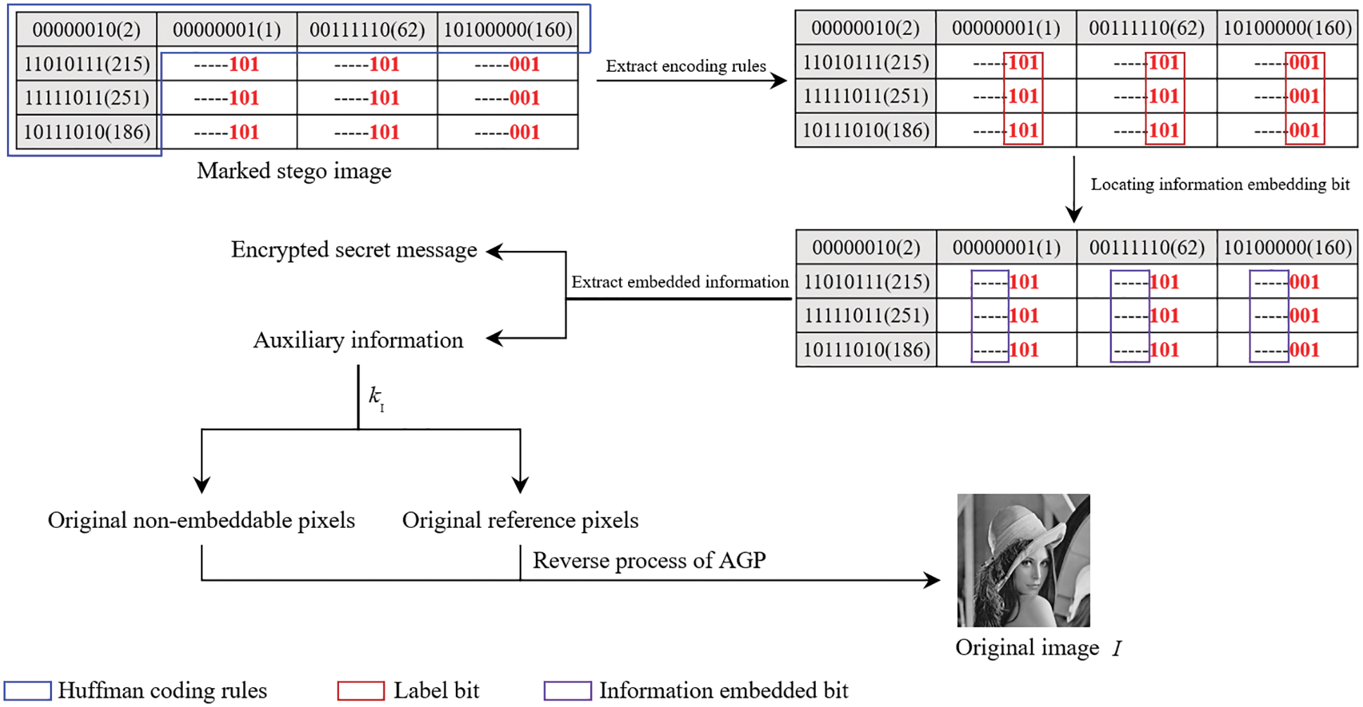
Figure 9: The process of image recovery

3  Experimental Results and Analysis

Experimental environment: MATLAB R2019a; Experimental setup: we test the effect of different thresholds on the performance (see in Section 3.1), the comparison and analysis with other schemes [22–25] (see in Section 3.2), the security analysis of our scheme (see in Section 3.3).

Metrics: the embedding rate (ER, expressed in bits per pixel (bpp)), the average embedding rate, Point Signal Noisy Ratio (PSNR), and Structural Similarity (SSIM).

3.1 Threshold Selection Experiment

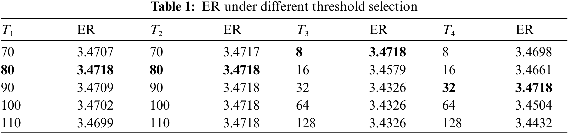
From Section 2.1.1, we know that AGP needs to adjust the threshold according to the edge case where the pixel is located. Therefore, to verify the effectiveness of the threshold, we take the Lena image as an example and conduct the threshold selection experiments shown in Tab. 1.

It can be seen from Tab. 1 that when the predicted pixel is at a sharp edge, the embedding rate is optimal when T1 is 80 and T2 is 80. Similarly, when it is on a non-sharp edge, the scheme’s performance is optimal when the threshold T3 is 8 and T4 is 32.

3.2 Analysis of Embedding Performance

To verify the embedding performance of our scheme, we first select six standard grayscale images of Lena, Man, Jetplane, Baboon, Tiffany, and Airplane shown in Fig. 10 for embedding rate experiments. To further verify the generality of the scheme, we conduct average embedding rate experiments on UCID [27], BOSSbase [28], and BOWS-2 [29].

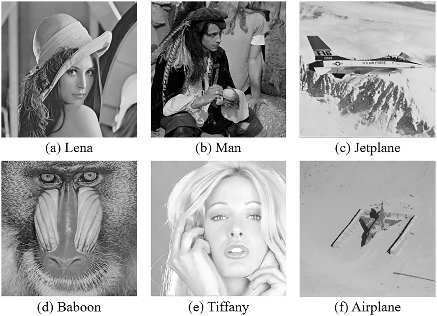
Figure 10: Six standard grayscale images

The comparison results of our scheme and different methods on six images are shown in Fig. 11. Our scheme outperforms other schemes [22–25]. Taking the Jetplane image as an example, the embedding rate of our algorithm is 1.5525, 0.9679, 0.6102, 0.2385 bpp higher than [22–25], respectively. Since Wu et al. [23] uses MED with a smaller receptive field for prediction, the perception ability of complex images is insufficient, thus affecting the overall embedding performance of the scheme. Yin et al. [24] use the predefined huffman coding, but for different images, the unified huffman coding is not the best coding rule, which leads to a decrease in the embedding rate. Our algorithm utilizes the pixel correlation of the whole image. It improves the prediction accuracy of the predictor for pixels in the texture area of the image through four scanning methods. At the same time, adaptive huffman coding is used to generate huffman codewords for different images adaptively, so the embedding rate is higher.

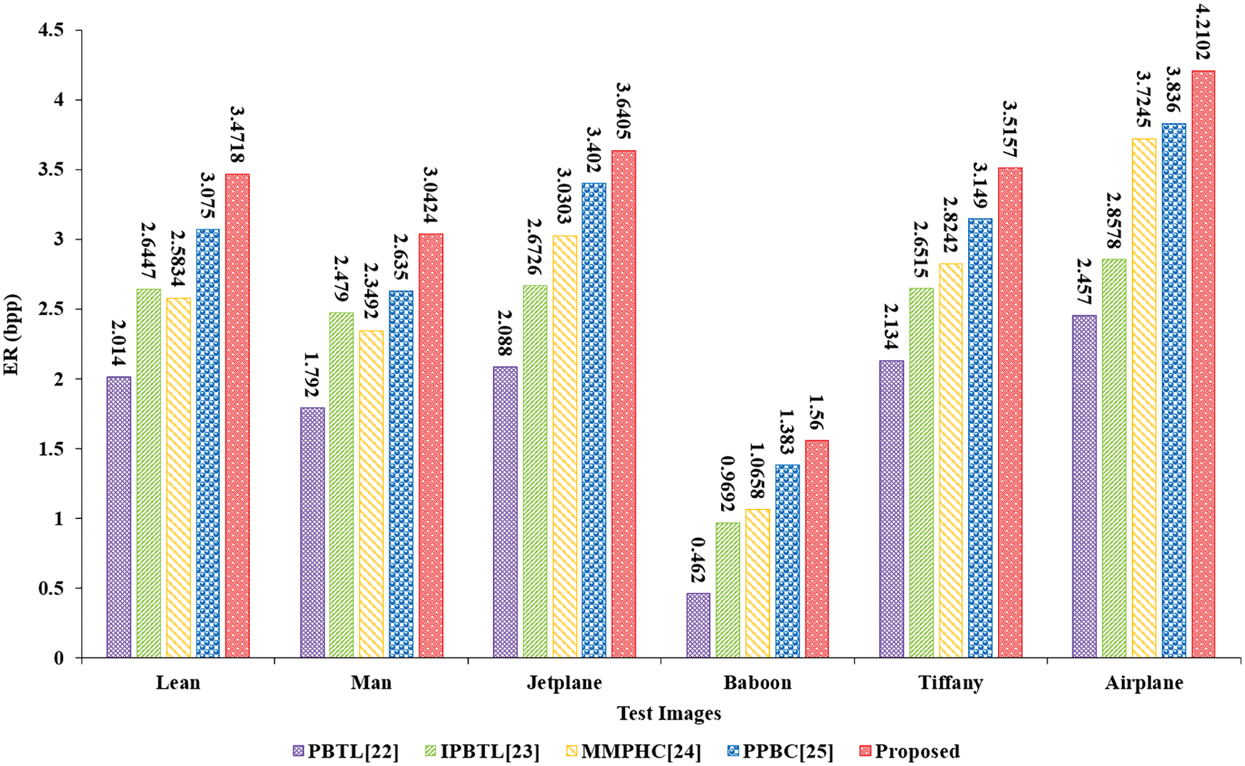
Figure 11: ER (bpp) comparison of different methods on six test images

In Fig. 12, we compare the average embedding rate of our scheme with different methods on three datasets. The average embedding rate of our scheme is higher than [22–25]. Specifically, our scheme achieves an average embedding rate of 3.5160 bpp on three datasets. While the literatures [22–25] are 1.808, 2.4497, 3.0983 and 3.3397 bpp respectively, we have an increase of 94.5%, 43.5%, 13.5% and 5.3%.

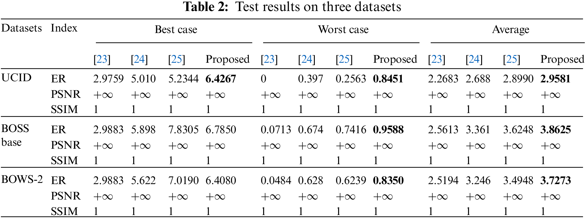
To further verify the advantages of our scheme, we test the embedding rate (bpp), PSNR (dB), and SSIM of different schemes in three datasets, results are shown in Tab. 2. Since scheme [22] is older and scheme [23] is an improvement of the scheme [22], we only compare this scheme with schemes [23–25] in detail. Where PSNR=+∞, SSIM=1 means that the recovered image has the same structure as the original image, and our scheme can recover the original image losslessly. Since AGP can combine the edge features of the predicted pixels and achieve better prediction results, the worst embedding rates on the three datasets are significantly improved. The scheme has better embedding performance on complex images.

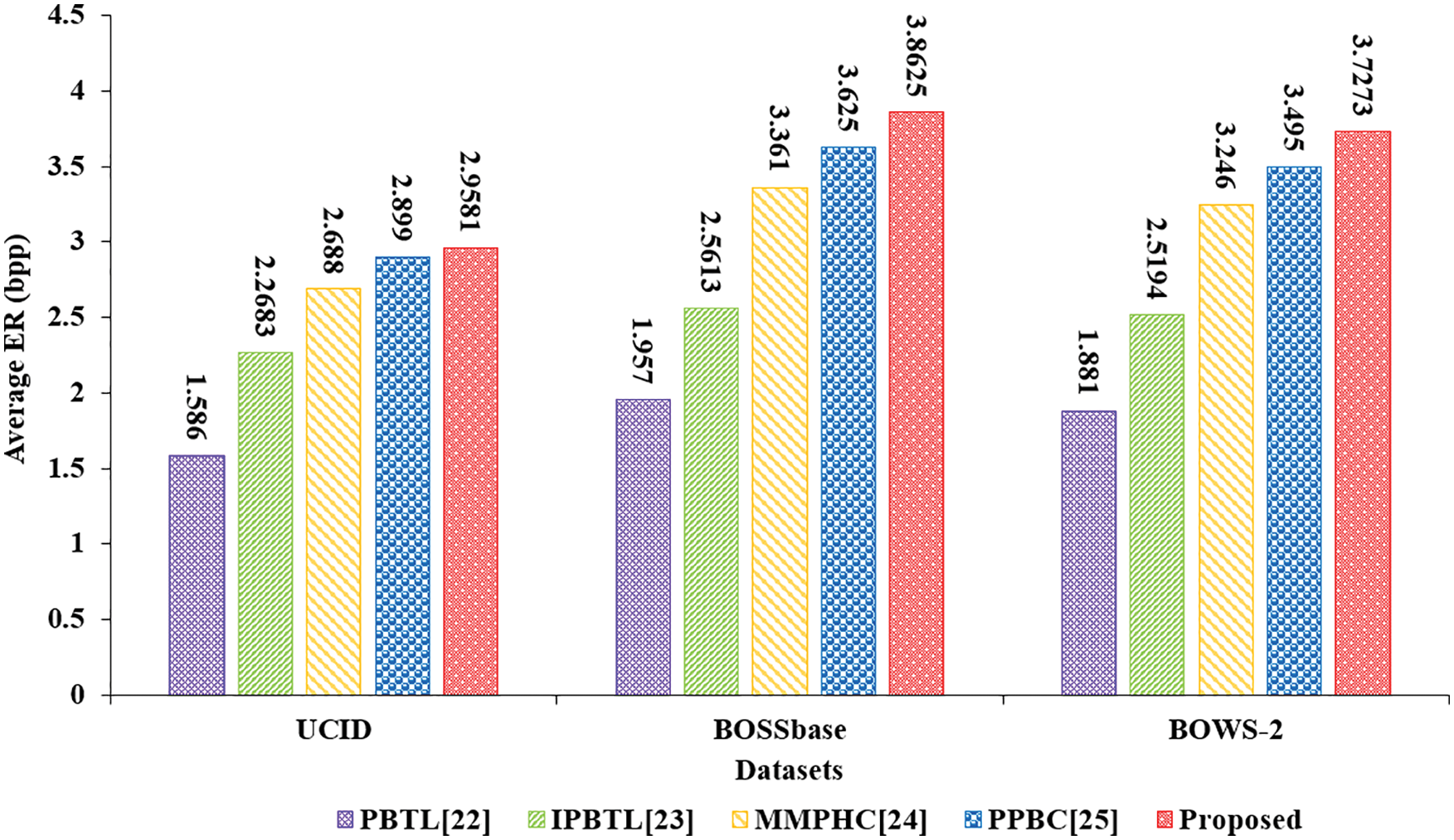
Figure 12: Average ER (bpp) comparison of different methods on three datasets

3.3 Safety Performance Analysis

This section first shows the stage image of the original image in the process of reversible data hiding, then compares the distribution of image histogram before and after encryption, and finally gives the results of common security indicators to illustrate the algorithm’s security. Fig. 13 shows the results of Peppers after encrypting, embedding data, and recovering.

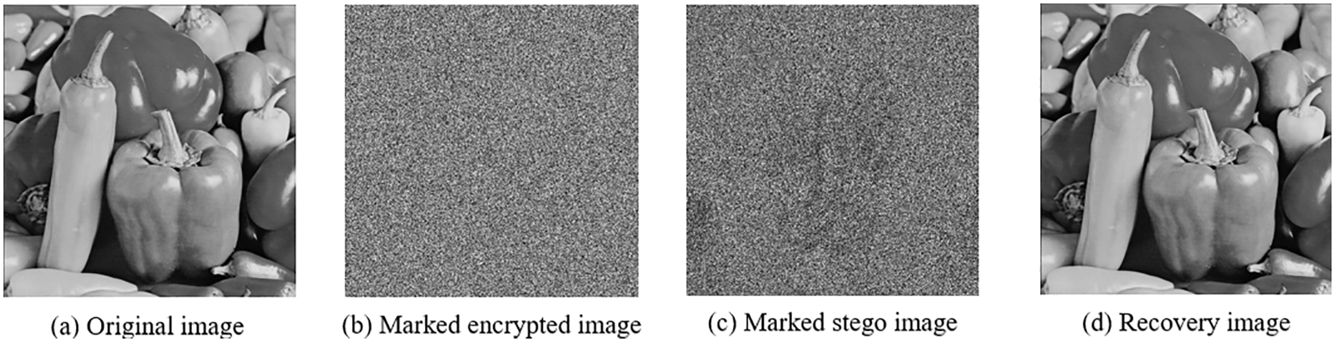
Figure 13: The results of peppers after encrypting, embedding data, and recovering

The histogram distribution of each stage of Peppers is shown in Fig. 14. The histogram containing the original image information is displayed in Fig. 14a. The histogram after stream cipher encryption is shown in Fig. 14b. The pixels are uniformly distributed, and the feature information of the image cannot be obtained. The histogram after embedding the data is shown in Fig. 14c. The content of the original image cannot be obtained from the encrypted image. The above experiments verify that the algorithm has good security performance and can resist standard cryptographic attack methods, such as statistical analysis attacks.

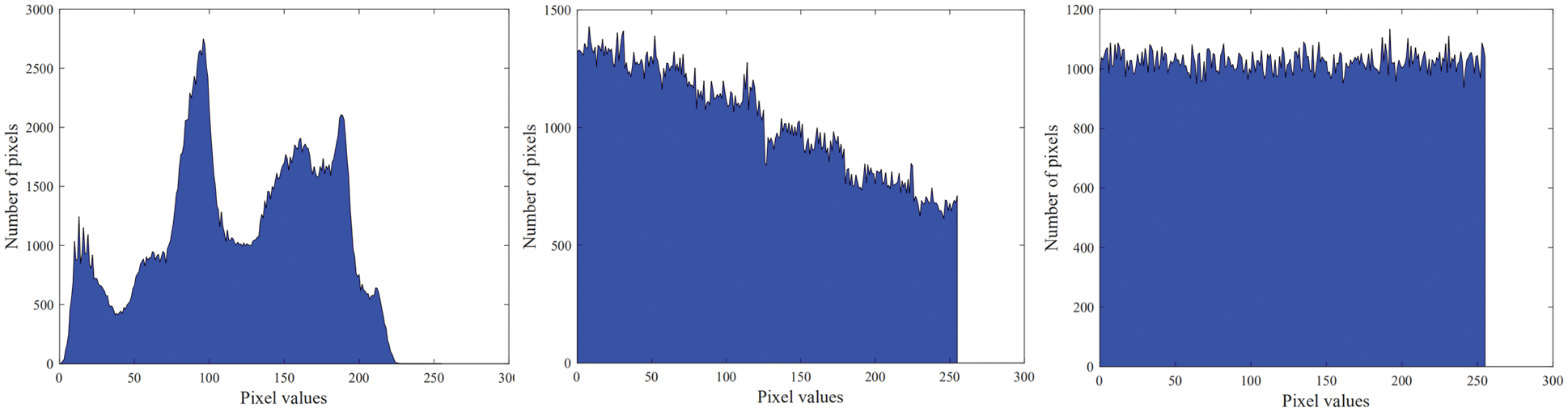
Figure 14: Histogram distribution of each stage of peppers

To further verify the algorithm’s security, Tabs. 3 and 4 shows the PSNR and SIM of the scheme on six standard grayscale images.

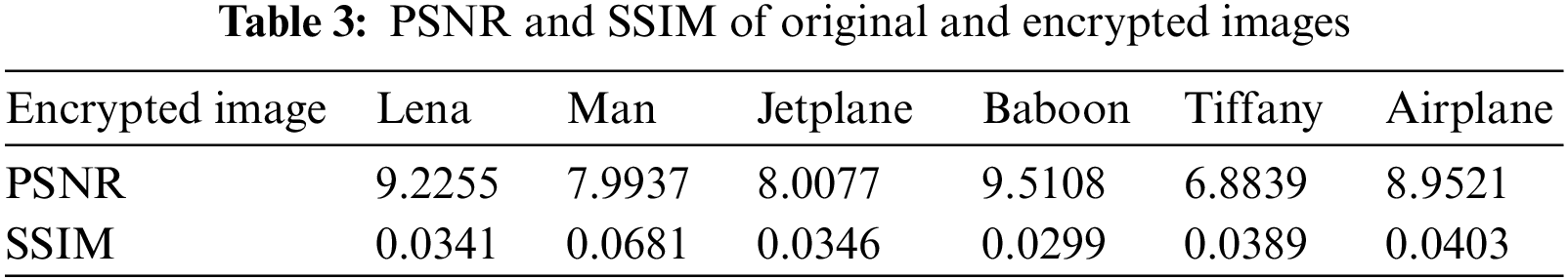
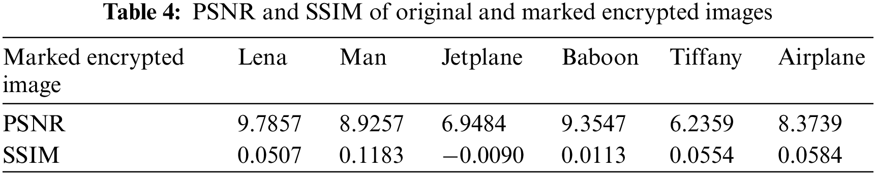
As shown in Tabs. 3 and 4, the PSNR of both the encrypted and marked encrypted images are very low, and their SSIM are almost 0. Therefore, the information of the original image cannot be obtained from the encrypted version image, which means that the proposed method safely protects the privacy of the original image and can be applied to RDH in the encrypted domain.

4  Conclusion

In this paper, we propose an RDHEI algorithm based on adaptive gradient prediction (AGP) and code labeling. An adaptive gradient predictor is proposed to aim at the multi-directional requirement of texture attributes in natural images. AGP can adaptively adjust the weights of the four scanning methods to predict the target pixel according to the texture features around the pixel. This method combines the advantages of AGP and adaptive huffman coding and reserves more space for data embedding. Compared with existing RDHEI schemes, our scheme provides a higher embedding rate while ensuring that the receiver can accurately extract the secret information and recover the original image without image quality degradation.

Funding Statement: This work was supported in part by the Natural Science Foundation of Hunan Province (No. 2020JJ4141), author X. X, http://kjt.hunan.gov.cn/; in part by the Postgraduate Excellent teaching team Project of Hunan Province under Grant (No. ZJWKT202204), author J. Q, http://zfsg.gd.gov.cn/xxfb/ywsd/index.html.

Conflicts of Interest: The authors declare that they have no conflicts of interest to report regarding the present study.

This work is licensed under a Creative Commons Attribution 4.0 International License, which permits unrestricted use, distribution, and reproduction in any medium, provided the original work is properly cited.