DOI:10.32604/cmc.2022.030418
| Computers, Materials & Continua DOI:10.32604/cmc.2022.030418 | |
| Article |
A Computer Vision-Based Model for Automatic Motion Time Study
School of Manufacturing Systems and Mechanical Engineering, Sirindhorn International Institute of Technology, Thammasat University, Pathum Thani, 12120, Thailand
*Corresponding Author: Warut Pannakkong. Email: warut@siit.tu.ac.th
Received: 25 March 2022; Accepted: 07 May 2022
Abstract: Motion time study is employed by manufacturing industries to determine operation time. An accurate estimate of operation time is crucial for effective process improvement and production planning. Traditional motion time study is conducted by human analysts with stopwatches, which may be exposed to human errors. In this paper, an automated time study model based on computer vision is proposed. The model integrates a convolutional neural network, which analyzes a video of a manual operation to classify work elements in each video frame, with a time study model that automatically estimates the work element times. An experiment is conducted using a grayscale video and a color video of a manual assembly operation. The work element times from the model are statistically compared to the reference work element time values. The result shows no statistical difference among the time data, which clearly demonstrates the effectiveness of the proposed model.
Keywords: Motion time study; computer vision; convolutional neural network; manual operation; standard time
In the age of Industry 4.0, manufacturing companies implement digital technology such as computer vision, Internet of Things (IoT), and big data to improve their ecosystem [1]. An important essence of a company’s profitability is cost management. There are various ways that a company can improve its cost management, and one of the most critical areas is production planning. An effective production planning can reduce inventory, shortage, and operational costs. Many developed countries started to implement some level of automation into their manufacturing processes, resulting in a consistent and predictable processing time. However, many developing countries lack the resources and knowledge to transform their manufacturing industry to automation and still rely on the human workforce in their daily operations. Unlike machines, manual operations’ processing times by human operators are naturally inconsistent. Therefore, time study is needed to find the standard time of manual operation.
A processing time is the elapsed time between the start and finish of an operation. An operation may consist of many work elements, each of which are defined either from the operator’s motion (i.e., holding, releasing, or grabbing an object) or changing in the shape of a workpiece from a manufacturing operation (i.e., a lathe machine transforming an ingot into a rod). Once multiple cycles of the operation are observed and processing times are recorded, the data can be used to determine the standard time. Standard time is the time required by an average skilled operator that is working at a normal pace to perform a manual operation. As the observed processing times can be different from cycle to cycle due to natural variability and working condition, the standard time represents the average time under a normal working condition. In addition, standard time calculation includes appropriate allowances, expressed in percentage of the observed time, that takes into account human factors such as rest to overcome fatigue, as well as performance rating factor that represents the relative working speed of operators to a normal pace.
Accurate standard time is essential for effective production planning and process improvement. If the standard times can be accurately determined, the production rate and resources can be appropriately prepared and allocated to minimize the risk of over and under-production, as well as overtime and idle time of human operators. Overproduction can result in excessive inventory and underproduction can result in shortages, while overtime results in high labor cost and idle time reflect over-staffing or unbalanced workload among operators. By comparing each operator’s processing time to the standard time, the company can clearly identify potential areas of improvement. Work elements of an operation that contributes the most to the overall processing time and its variability can be identified and improved upon.
Traditionally, time study requires an analyst to manually observe, time, and record several work elements comprising an operation using a stopwatch, which is naturally prone to errors. The errors may be caused by the analyst’s boredom and loss of focus from monotonous timing, not enough sample size (i.e., number of cycles to observe) of an operation, and operation disruption from various unavoidable factors. As humans are susceptible to boredom, repetitive actions can cause an operator to lose focus while performing the timing activity, which leads to inaccurate timing.
A long period of observing and timing can also lead to fatigue, which causes uncertainty and inconsistency in each timing instance. External factors such as noises, the operator being interrupted, or the operator switching to do other tasks during an operation cycle can also distract the analyst’s timing activity. As it is not financially viable to time every cycle of an operation, analysts have to observe the operation for an adequate number of cycles to carry out the time study. Observing an operation in real-time may cause some bias and make the observed cycles unrepresentative of the true operation. For example, operators may work unnaturally faster (or slower) when they are being observed and timed to meet the working standard (or to make the work appear as if it requires longer operation time). But when the timing is finished, the operators return to work at their normal speed. Uncertain processing time data lead to ineffective production planning, as the planning and management team cannot estimate the expected production output accurately.
Fortunately, with the emergence of machine learning, these mundane time study activities can be automated using computers. In this paper, a computer vision-based time study (CV-TS) model is developed to automate the time study process, thus eliminating the need for human analysts to manually perform time study. We demonstrate that the proposed CV-TS model can effectively perform this task and completely remove timing uncertainty, therefore, allowing the analysts to focus on other non-mundane and creative tasks such as operation improvement.
Contributions of the paper are three-fold. First, we successfully develop a computer vision model that can analyze the video of an operation and automatically detect and classify work elements that comprise the operation. Second, we integrate the computer vision model to a time study model that takes the outputs from the computer vision model as input and performs time study automatically. Finally, we demonstrate the effectiveness of the proposed model using video of a manual assembly operation.
Computer vision is a field of artificial intelligence that trains computers to interpret and analyze the visual world through images. Computer vision algorithms allow computers to process visual data, giving them the ability to identify objects in still and moving images (i.e., video). Many organizations now collect data from a variety of sources, such as smart devices, industrial equipment, videos, social media, and business transactions. The proliferation of available data accelerated artificial intelligence development such as computer vision algorithms that allow computers to detect objects with higher speed and accuracy.
Various research studies explore industrial applications of computer vision. The most prevalent applications are measurement and quality control. An example of an application to quality control is the study conducted by Kazemian et al. [2]. The authors built a system using computer vision algorithms to control and monitor the quality of an extrusion process. By utilizing image binarization and blurring for contour extraction, the computer vision system can produce reliable feedback. The extrusion rate is then adjusted automatically to maintain the quality of the extrusion process. Frustaci et al. [3] present another system using computer vision algorithms to check the assembly processes’ quality. Their proposed system can detect potential geometrical defects. They can achieve this by combining image processing techniques such as binarization and Region of Interest. An application of measurement using computer vision is demonstrated by Gadelmawla [4]. The author proposed a computer vision algorithm that can classify different types of threads and screws by comparing the extracted features from the images to their corresponding labels.
In recent years, the development of artificial neural networks (ANN) has made the field of computer vision popular. ANN models are capable of classifying images more accurately and quickly by utilizing a large amount of available data. An example of a computer vision system using ANN is shown in a study by Arakeri et al. [5]. A fruit grading system using computer vision is developed to evaluate and classify tomatoes. The system extracted features from tomato images and input them into an ANN model that determines if a tomato is ripe, unripe, or defective. The system can process up to 300 tomatoes per hour. The throughput of the image classification system was improved further by Costa et al. [6]. The authors were able to increase the processing speed to 172,800 tomatoes per hour. The introduction of a residual neural network (ResNet), a variant of convolutional neural network (CNN), has been credited for the significant improvement of the processing speed. CNN has a similar model structure to the classical ANN as they both contain self-optimize neurons through learning [7]. CNN has become popular in recent years due to its effectiveness in object detection. Prominent applications such as surveillance, self-driving cars, and object counters use CNN to detect objects.
The main difference between ANN and CNN is that CNN is mainly used for pattern recognition in images. A CNN model can capture patterns and spatial features from images and encode the features into the model architecture. This allows the model to perform better in image analysis tasks and requires fewer parameters than ANN. An example of a use case of CNN is presented by Raymond et al. [8], where the authors designed a system that manages electrical grid assets such as transformers, insulators, switches, and supports by using Faster-RCNN, a variant of CNN. Drones are used to take pictures of the assets and the images are input into the Faster-RCNN model. The model counts the assets from the images and finally generates an inventory report. In the field of transportation, [9,10] utilized CNN to identify vehicles. As more studies and applications use CNN to solve real-world problems, the evidence of CNN’s effectiveness is further solidified.
Although the use of computer vision in motion time study can be classified as one of the Industry 4.0 methods in improving process timing according to Liebrecht et al. [11], there is a limited number of studies under this research area. Recently, Ji et al. [12] developed a computer vision algorithm that can perform motion time study automatically. However, the work process in the video analyzed in the study is simple and the procedure in developing the time study model lacks an in-depth description. This paper is a significant extension of Ji et al. [12]. The discussion of the model’s parameters, model development, and steps in automatically performing motion time study with computer vision is expanded. Image augmentation is introduced to increase the model’s generalization. In addition, the results from the model are further explained to strengthen the study’s contribution.
Certainly, there are various ways in detecting an operator’s motions. The use of sensors to recognize activities has been reviewed by Wang et al. [13]. The authors explained how traditional activity recognition methods mainly rely on manual heuristic feature extraction, which could impede their generalization effectiveness. Some research studies found success using motion sensors to recognize the activity. However, sensors can interfere and obstruct the operators’ movement or vice versa, thus affecting their respective performance. Therefore, in our work, we choose to perform a time study by utilizing cameras with computer vision algorithms instead of sensors as they do not interfere with the operators’ movement and can detect objects with better accuracy and from further range. The implementation cost and setup complexity of cameras tend to be significantly lower, as the equipment needed is only a video camera and a computer to run the model’s algorithm. The specification of these equipment depends on the complexity of the operation and desired accuracy of the time result. A video camera with a higher specification can capture more pixels in a video frame, therefore, providing more information to the model. A model that has been trained with a larger amount of data, in this case, images with more pixels, is less susceptible to false-positive detections. A computer with higher specifications can process videos faster and potentially can run the model in real-time.
In recent years, many research papers explore methods in detecting motion using computer vision. Huang et al. [14] proposed a method based on pose estimation and region-based CNN. The pose estimation is used to obtain the trajectory information of the human joints and the CNN is used to predict whether the workbench is empty or not, increasing the accuracy. The method is demonstrated on a hand sewing process video by counting the number of products. Sun et al. [15] developed an automatic system to monitor and evaluate a worker’s efficiency. The authors used generative adversarial networks with pose estimation to detect human body joints. The video of an action performed by a worker is matched against a reference video performed by a teacher using pose estimation and temporal action localization to obtain efficiency. Mishra et al. [16] proposed a Fuzzy inference system with CNN for human action recognition. Ullah et al. [17] also proposed an action recognition system that utilizes CNN, deep autoencoders, and quadratic support vector machines algorithm to learn temporal changes of the actions in a video stream. From our findings, utilizing CNN in action recognition has been popular. However, to the best of our knowledge, studies that implement CNN in the motion time study applications are limited [18]. This study proposes a motion time study model that utilizes CNN to automatically conduct a time study on a video of a manual operation.
Computer vision is a field of artificial intelligence that trains computers to interpret and analyze the visual world through images. Computer vision algorithms allow computers to process visual data, giving them the ability to identify objects in still and moving images (i.e., video). Many organizations now collect data from a variety of sources, such as smart devices, industrial equipment, videos, social media, and business transactions. The proliferation of available data accelerated artificial intelligence development such as computer vision algorithms that allow computers to detect objects with higher speed and accuracy.
A manual manufacturing operation usually consists of several work elements, each of which is further comprised of a sequence of motions. To determine each work element time, a time study analyst observes and detects the element’s starting and ending conditions by using distinctive sound, sight, and/or motions (i.e., movement of operator’s body parts). The analyst usually uses a stopwatch to time each work element by observing the manufacturing operation in real-time or by viewing a video clip of the operation. All work element times are combined to obtain the total observed operation time. The observed time is then adjusted by allowance (i.e., percentage of additional operation time required by human factor) and rating (i.e., the relative speed of operators to a normal pace) to give the final standard time of the operation. The time study activity requires a well-trained analyst observing a representative operator performing the operation for several cycles, followed by some clerical calculation to obtain the standard time. Our proposed method aims to replace this tedious time study process with a computer vision-based model that can automatically analyze video clip(s) of an operation and return a more accurate standard time than a human analyst. The model is an integration of two models: a computer vision model and a time study model.
The computer vision model implements the CNN model to perform video frame (or image) classification. As images are represented as pixel values, changes in the patterns of the pixel values can be easily identified by the model. Grayscale images in Fig. 1 simply illustrate this idea.
From Fig. 1, when the operator’s arm moves, the patterns of the pixel values also change, therefore, a change in action or motion can be detected. A grayscale pixel value ranges from 0 to 255. The pixel values closer to zero represent the darker shade, while the values closer to 255 represent the lighter or the white shade. In Fig. 1a, the pixel values of 200 that are clustered at the center of the highlighted area represent the operator’s left arm. Once the operator moves his arm to the center of the video as shown in Fig. 1b, the pixel values of 200 that represent the operator’s left arm moves to the right of the highlighted area (i.e., the center of the workbench). A colored image uses the same logic but with three times the amount of pixel values as a grayscale image because of the three different color channels in the image: red, green, and blue (see Fig. 2).
A CNN model has been proven to be appropriate for this role in detecting patterns in an image. The CNN model in this study aims to detect the work element to which a motion in a video frame belongs. That is, the output from the CNN model is the classification probabilities of each work element for a given video frame. The time study model then analyzes the CNN output to record the time when there is a change in the classified work element of a video frame to the next video frame. The CNN models to process the grayscale and color images are trained and their results are compared to check whether processing grayscale and color videos yield significantly different results.

Figure 1: (a) Pixel values of a work element in a still image from a video of an operation; (b) Pixel values of another work element in a still image from a video of the same operation

Figure 2: The pixel values of the highlighted area in the color image
Originally, our CNN model has a similar structure to the model developed by Goodfellow et al. [19]. However, since the CNN model analyzes each video frame (a single still image) independently, there is a “flickering effect,” where the classification of work element changes often from multiple video frames within the same work element. As a result, the element time cannot be recorded accurately. To overcome this problem, we implement the rolling-prediction averaging [20] in the time study model to improve the work element classification accuracy of video frames. We referred to our implementation as rolling-classification averaging.
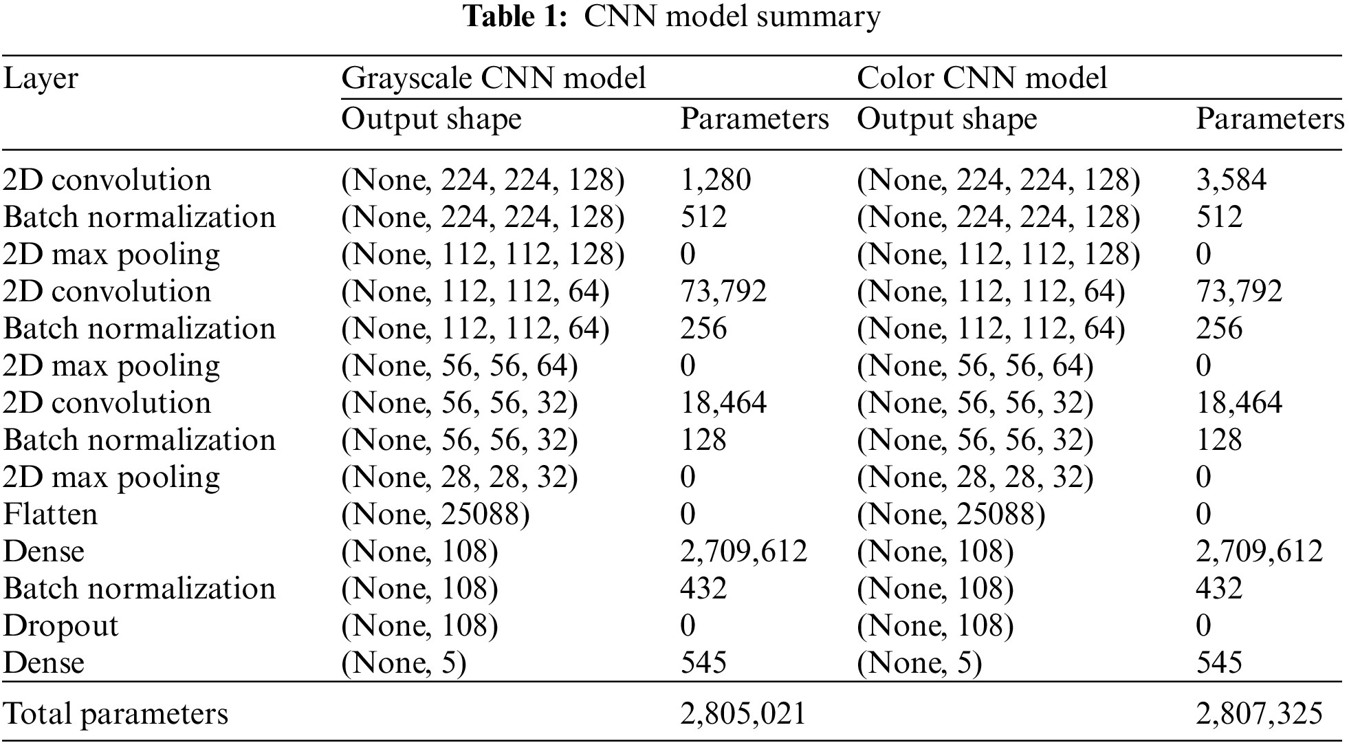
Our model development consists of two steps. First, the CNN model is trained to classify the work element of a video frame. Then, the time study model that implements rolling-classification averaging is constructed to find each work element time based on the classification output of the CNN model. The structure of the developed CNN models is summarized in Tab. 1. The CNN models to detect color and grayscale images have the same model architecture, with a slightly different number of trainable parameters. The two-dimensional (2D) convolutional layers apply filters to extract features. Batch normalization normalizes the outputs of the preceding convolutional layers to avoid overfitting of the model. The 2D max pooling layers then reduce the dimensionality of the network. Finally, the fully connected layers take the information from previous layers and aim to classify the input image. The outputs of the CNN model are the classification probability of each class, i.e., work element in this application.
The CNN training procedure is illustrated in Fig. 3. A video of a manufacturing operation is recorded by a camera. After recording, the video file is converted into individual still images or frames. A human modeler, with the knowledge of the conditions of the endpoint of each work element, then watches the video to approximate the times in the video that the changes of work elements occur. The video is rewatched on a frame-by-frame basis to accurately determine the timings of the endpoints of the work elements. All video frames that precede an endpoint can, therefore, be accurately labeled with the corresponding work element that they belong to. The manufacturing operation in this paper consists of four work elements. Thus, there are five label classes: four work elements and one element representing the operator being idle. After labeling all individual images, the images are separated into training and test sets. The CNN model is trained until the accuracy of classifying the images stagnates or there are signs of overfitting. Finally, the classification performance of the trained CNN model is evaluated using the test set.

Figure 3: CNN model training procedure
3.2 Computer Vision-based Time Study Model
The CV-TS model, which contains the previously trained CNN model in its architecture, is then constructed. The flowchart of the CV-TS model is shown in Fig. 4. The training procedure of the model starts by obtaining the video of the work process and initializing the following parameters: frame f, element i, cycle n, and timestamp of each element ti. The timestamp ti, obtained by the CV-TS model, has the index i that indicates the work element index. That is, t0 is the start of the first element, t1 is the end of the first element time and the start of the second element, and so on. Note that at the end of the last element of each cycle, the index is reset to t0 again. The recorded values of the timestamps are relative to the length of the video. It is the time of frame f at which the CV-TS model determines that an element has ended. All frames f from the video are inputted into the trained CNN and are sequentially processed to obtain the classification probability of each element.

Figure 4: The procedure of the CV-TS model
Next, the rolling-classification averaging is applied to improve the work element classification accuracy and eliminate the flickering effect that might occur if individual frames are independently analyzed instead. The average probability of each element from K latest frames is calculated. K is a hyperparameter that characterizes the sensitivity of classification. A high value of K makes the CV-TS model less sensitive to the change in motions, which can lower the chance of incorrect classification. Nevertheless, a too high value of K can result in an insensitive model that does not classify any difference in work elements and ends up with the same classification for every frame, which makes the CV-TS model ineffective. On the other hand, a low value of K makes the CV-TS model more sensitive to the change in motions, resulting in higher timing accuracy, but more susceptible to the flickering effect that leads to incorrectly classifying the work elements. Specifically, the flickering effect occurs when the classification of the model incorrectly switches rapidly between two labels in the video on subsequent frames. The optimal value of K varies and depends on the complexity and time duration of the work elements.
Moreover, a video with higher frame rate tends to show smoother motion from frame to frame. In other words, two consecutive video frames are quite similar to each other, therefore, a higher value of K may be needed. On the other hand, a video with lower frame rate tends to show less smooth motion where two consecutive video frames are relatively different from each other. Therefore, a higher value of K can yield inaccurate results. Finding an appropriate value of K for a given video with a specific frame rate for an operation requires a tuning process to find the optimal K. In this process, various values of K should be tested and the value that yields the most satisfactory results should be selected. A comprehensive relationship between K and the video’s frame rate is not explored in this study. The provided explanation is only a guideline on how to set the initial parameter K.
In this study, values of K in the range of 30 to 80 with an increment of 5 are tested to find a suitable value of K. Time study is performed with 11 values of K and the obtained time (Ei,n) of element i in cycle n of each K is compared to the reference time (Ri,n) of element i in cycle n to find the mean absolute error (MAE), shown in Eq. (1). The reference time is obtained by an expert that manually times the operation in the video in slow motion on a frame-by-frame basis to record the element times as accurately as possible. In this case, the reference times represents the best possible values that an operator can obtain when performing the time study. The MAE from different values of K are compared and the K that results in the lowest MAE is chosen to be used in the final time study model. The MAE of each K tested is plotted in Fig. 5. It is found that the K value of 60 frames results in the minimum MAE.

Figure 5: The MAE of each hyperparameter K
The work element with the largest average probability is chosen as the classification of the current frame that is analyzed, hence, the so-called rolling-classification averaging. Finally, the classification of the current frame that has been obtained from the rolling-classification averaging is compared to the previous frame’s classification. If both classifications are the same, then it is considered that the current classified work element is still ongoing and the timing continues. Otherwise, it is considered that the previous work element has ended and a new work element has begun, at which point the timestamp ti is recorded. The timestamp ti is the cumulative time of the processed video, with the initial timestamp t0 = 0. Once a cycle ends, t0 is set to the current timestamp when the cycle ends. The time (Ei,n) of element i in cycle n is calculated by taking the difference between the current timestamp ti and the previous timestamp ti−1, shown in Eq. (2). A new cycle starts when the time of the last element in the cycle has been calculated. Every frame of the video is processed sequentially until the last frame of the video has been analyzed, all work element times are then recorded and a data file is generated.
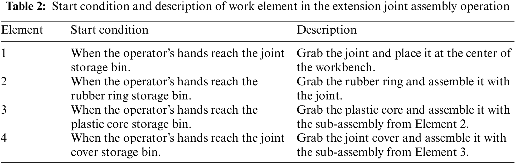
In this section, the CV-TS model’s performance is evaluated using a 352 × 288 pixel video footage of an extension joint assembly operation (see Fig. 6). The video was originally recorded to teach undergraduate students how to conduct a time study. The extension joint assembly operation contains four work elements. The start conditions of each element are defined in Tab. 2.
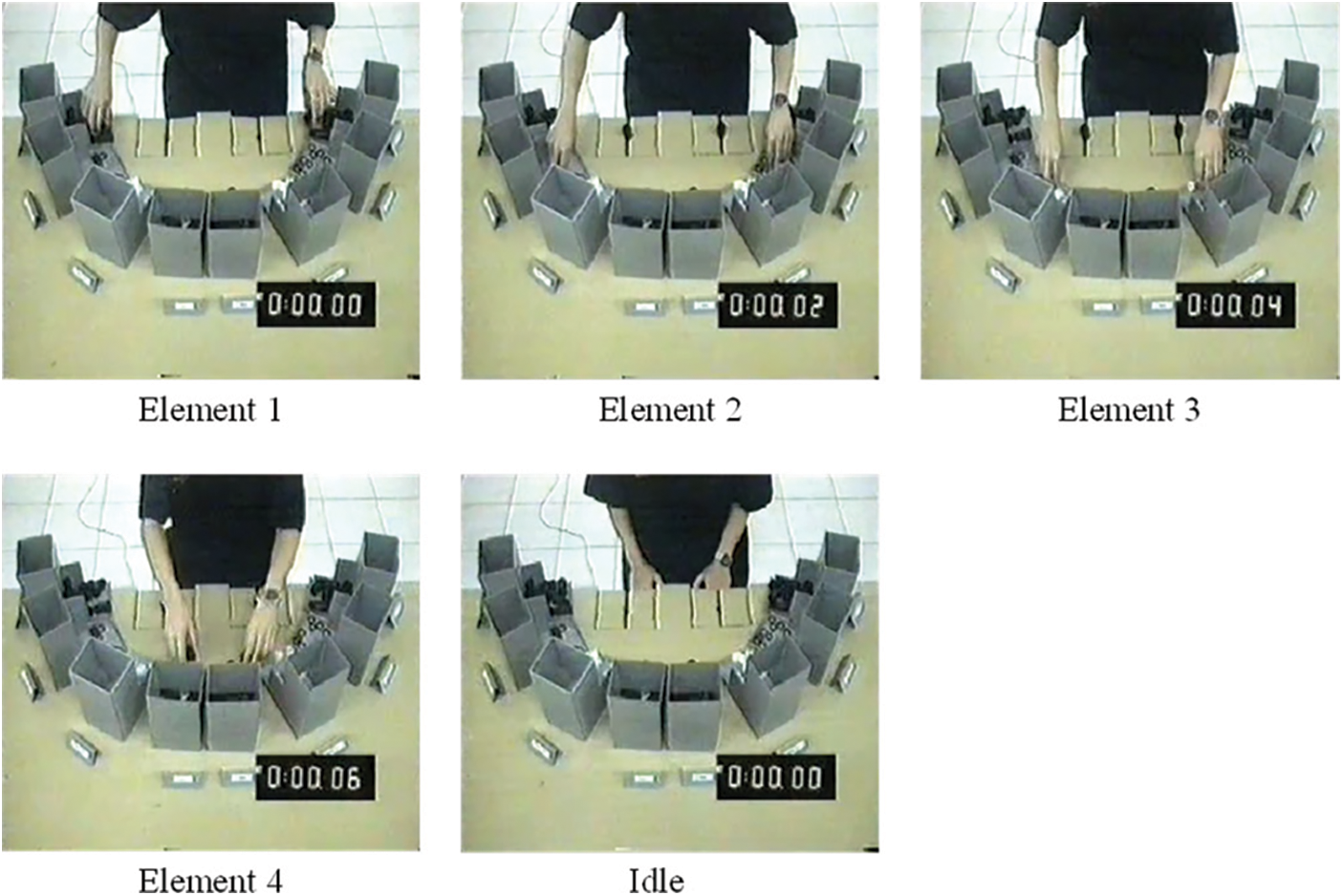
Figure 6: A frame of each work element from the extension joint assembly operation video
The video of the extension joint assembly operation contains 10 cycles. The operator performs each cycle in the same manner. The video has a resolution of 352 × 288 pixels and a frame rate of 25 frames per second. The length of the video is 2 min and 22 s. The video is converted into individual frames (images). It is not required to convert every frame in the video into an image, since doing so will produce many identical images and add unnecessary computation to the CNN model training process. Instead, video frames can be converted into images in an interval, for example, every 10th frame in the video. In this experiment, every 5th frame in the video is converted into an image, resulting in 710 images in total. To further demonstrate the applicability of the CNN model, the images from the video are modified so that they appear to the CNN model as if there are variations in the recording conditions, e.g., lighting, operator, etc. The image modification is performed by image augmentation, a technique to increase the diversity of the training set by applying random transformations [21]. Using this technique, the images are randomly cropped, rotated, and their brightness and contrast modified. The transformations were not drastic as the conditions in the manufacturing settings are usually consistent. After all the images are transformed, the images are split into the training and test sets, using the common 80/20 split. 80 percent of the images (568 images) are randomly assigned to the training set and the remaining 20 percent (142 images) to the test set and used to evaluate the trained CNN model. The implementation of image augmentation and train/test split is demonstrated in Fig. 7. The experiment was carried out on an Intel Core i7-9700K 3.60 GHz personal computer with 16 GB of RAM and NVIDIA GeForce RTX 2060 SUPER 8 GB GPU.

Figure 7: The procedure of image augmentation and train/test split
A stochastic gradient descent (SGD) optimizer [22] is used in the model training. According to a survey done on optimization methods by [23], SGD is one of the most popular optimization methods used in machine learning. It is used to find the model parameters that correspond to the best fit between actual and predicted outputs of the model. The training of the grayscale and color CNN models was performed for 50 epochs, at which point the training accuracies start to stagnate and both models’ training time was approximately five minutes (see Fig. 8). The accuracy of the grayscale and color CNN models on the image test sets were 86 and 89 percent, respectively. The classification evaluation metrics of the trained models are shown in Tab. 3.
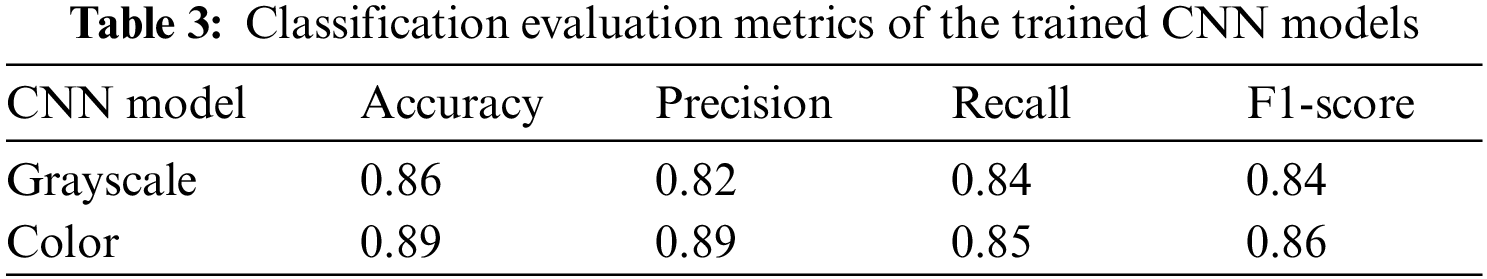
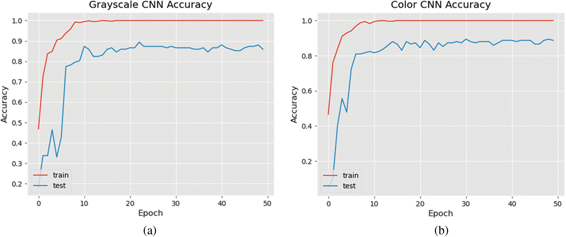
Figure 8: (a) Accuracy of the CNN model trained to detect the grayscale image; (b) Accuracy of the CNN model trained to detect the color image
The time study model is then constructed to automatically time the work elements by analyzing the classification outputs from the CNN model. After the two models are integrated, the video of the extension joint assembly operation is analyzed and the resulting element times are obtained in a format of a .csv data file. The processing times of the grayscale and color video are both approximately six minutes. The result is then compared with the reference time. In an ideal case, the work element times from the model should be the same as those of the reference time. A statistical test, analysis of variance (ANOVA), is performed to check whether there is a significant difference between the reference element times and the times obtained by the CV-TS model.
The video of the extension joint assembly operation is analyzed by the proposed CV-TS model, which generates two output files. The first output is the same video with additional work element time data annotated in the video frames. The annotation can help a human analyst to evaluate whether there are any misclassifications or timing errors (see Fig. 9). The video can be found in the “Data Availability Statement” section at the end of the paper.
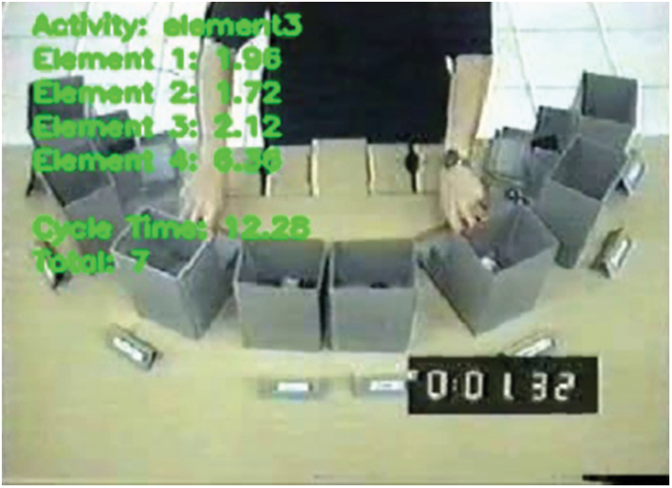
Figure 9: A sample frame of the video output from the model
The annotations display the following information: The classified work element of the current frame, most updated work element times and cycle time, and the cumulative number of cycles completed. The annotations allow the analyst to pinpoint the cause of the problem when irregularities are found in the time study data. For example, if the recorded time of Element 4 in Cycle 2 is found to be shorter than average, the analyst can view the video and see if the model correctly classified the work element by looking at the annotations. This may be caused by the camera view being obstructed or the operator accidentally dropping the workpiece, which leads to misclassification by the model. Although the annotations are the only display of the output (i.e., not a part of the model’s analysis), the annotations can help with the result verification and debugging process.
The other output is a .csv data file that contains the element times of each work cycle, along with each work element’s average time and standard deviation. The .csv data file is automatically generated by the time study model, which makes the time study process more convenient and removes the risk of human errors from manual data entry by the analyst. Tab. 4 contains the work element times from the model using color video and grayscale video as input files. In addition, the reference work element times of each cycle are shown in Tab. 4. The reference times are obtained by a human analyst watching the operation in the video in slow motion. Thus, the reference times represent the completely accurate time study results, where the start and the end of each work element are correctly identified. These results are otherwise, impossible to obtain if the time study were conducted in real-time, especially in the case where the motions are fast, which makes the timings difficult to accurately record.
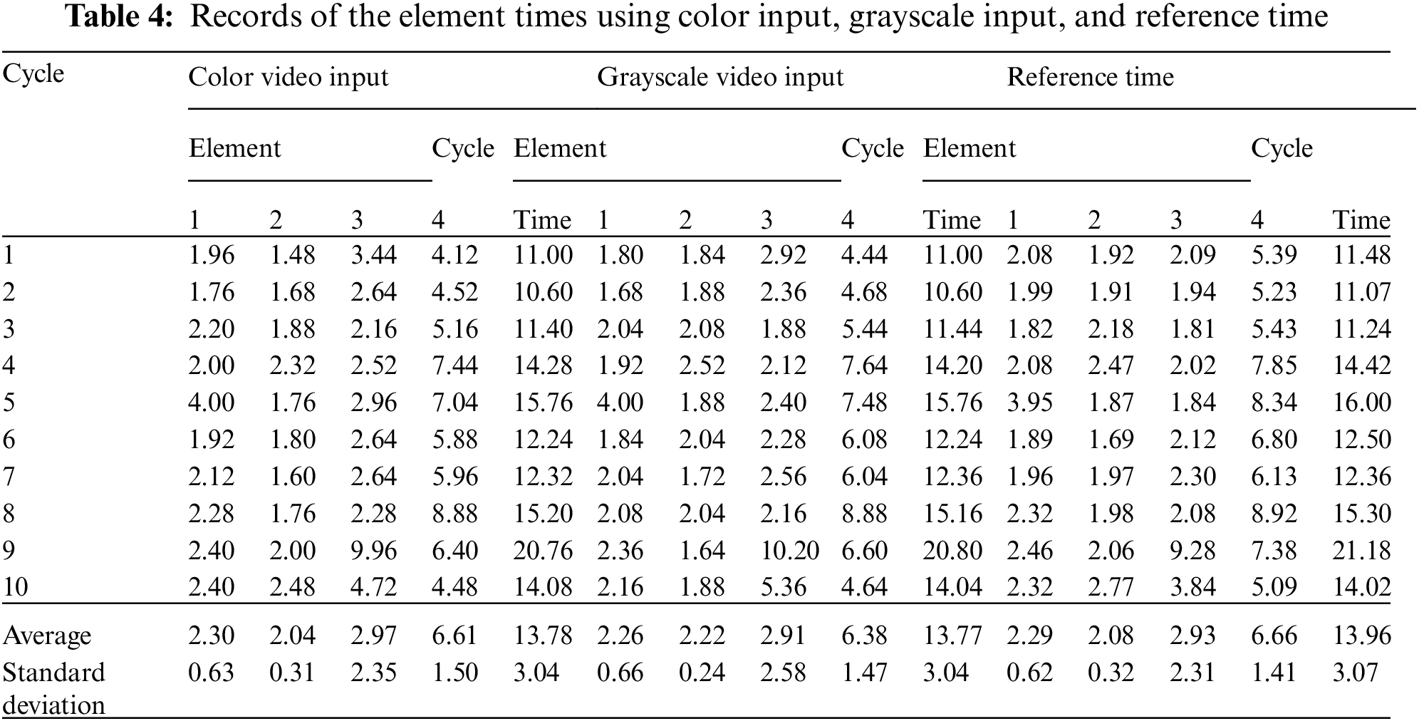
For example, the timestamps of the color video input are obtained as follows: at the start of the video (initial timestamp t0) is set to 0. When the first element of the first cycle ends, the timestamp t1 records the current time in the video, t1 = 1.96. The timestamping repeats until the last element of the first cycle has ended with a cycle time of 11.00 s, t0 is reset to the current timestamp of the video (t0 = 11.00 s). The work element time is estimated from the difference between two adjacent timestamps, e.g., the element time of element 1 is equal to t1 − t0 = 1.96 s.
To test the performance of the proposed CV-TS model, the element times obtained from the model are compared to the reference times. To evaluate the CV-TS model, we check if the element times obtained from the model are statistically different from the reference times. If the results are not statistically different, it is inferred that the CV-TS model can adequately perform an accurate time study. An ANOVA is performed to test whether there are statistical differences among the estimate times from the model and the reference times (see Tab. 5). The p-value from the ANOVA is used to check for the statistical significance. From the ANOVA, there are no significant differences between the average work element times obtained from the CV-TS model using color and grayscale inputs and those of the reference element times, p-value = 0.74. This indicates that the CV-TS model can accurately and adequately record the element times, which can lead to the correct standard time of the assembly operation. Note that the ANOVA is performed while taking into account the significant effects of the differences in the work elements and cycles. Naturally, different work elements require significantly different times to carry out, and the operator performance from one cycle to other cycles is not the same. Finally, Fig. 10 illustrates the correlation between the element times of the two methods, all pairs of correlation coefficients are at 0.997, indicating very high consistency between them.
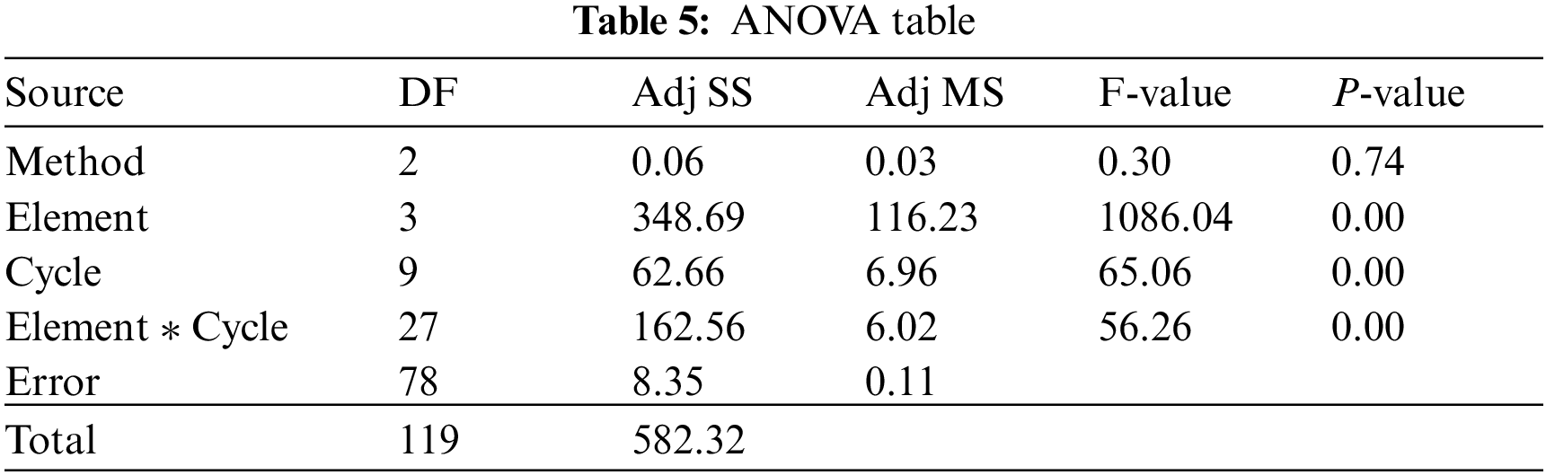

Figure 10: Correlation between element times from the two methods
A computer vision-based time study model that automatically records work element times, which are differentiated by operator’s motions, from a video is proposed in this paper. Based on the experiment, the model’s estimated work element times from grayscale video and color video are compared with the reference time. ANOVA result indicates no statistically significant difference among them. Therefore, it can be concluded that the proposed CV-TS model can perform a time study indistinguishably from the reference value. In addition, the computational power required to process color and grayscale videos is indifferent as the video size is small. The accuracies of the color and grayscale CNN are also relatively the same since the video of the operation has good contrast between the operators’ body parts and the surroundings. However, the computational requirement and accuracy can be significantly different in videos of other operations. Increasing the complexity of the operation or random noises in the video may reduce the model’s effectiveness, therefore other advanced variants of CNN may be required.
As future work, these issues will be further investigated. Random, unrelated, incorrect motions and less contrast background and surroundings will be deliberately introduced to the video of the operation. This is to test whether the model can accurately classify these motions and time the work elements. The complexity of the operation can also be increased, such as increasing the number of motions, work elements, and adding multiple operators.
The CV-TS model can yield accurate work element times that can be used to determine the standard time. Accurate standard time is essential for production planning and process improvement. Implementing the model can help companies eliminate the need for analysts to perform time studies manually. This allows the analysts to work on other creative tasks, such as identifying rooms for improvement, implementing solutions to improve the operations. In addition, the data can be integrated with other data obtained from IoT devices to perform further analysis to improve the system. Finally, there are numerous potentials and benefits from applying the proposed model to various manual operations in both service industries and labor-intensive manufacturing industries.
Funding Statement: This work is jointly supported by the SIIT Young Researcher Grant, under a Contract No. SIIT 2019-YRG-WP01, and the Excellent Research Graduate Scholarship, under a Contract No. MOU-CO-2562-8675.
Conflicts of Interest: The authors declare that they have no conflicts of interest to report regarding the present study.
1. J. S. M. Yuen, K. L. Choy, H. Y. Lam and Y. P. Tsang, “An intelligent-internet of things (IoT) outbound logistics knowledge management system for handling temperature sensitive products,” International Journal of Knowledge and Systems Science, vol. 9, no. 1, pp. 23–40, 2018. [Google Scholar]
2. A. Kazemian, X. Yuan, O. Davtalab and B. Khoshnevis, “Automation in construction computer vision for real-time extrusion quality monitoring and control in robotic construction,” Automation in Construction, vol. 101, pp. 92–98, 2019. [Google Scholar]
3. F. Frustaci, S. Perri, G. Cocorullo and P. Corsonello, “An embedded machine vision system for an in-line quality check of assembly processes,” Procedia Manufacturing, vol. 42, pp. 211–218, 2020. [Google Scholar]
4. E. S. Gadelmawla, “Computer vision algorithms for measurement and inspection of external screw threads,” Measurement, vol. 100, pp. 36–49, 2017. [Google Scholar]
5. M. P. Arakeri and Lakshmana, “Computer vision based fruit grading system for quality evaluation of tomato in agriculture industry,” Procedia Computer Science, vol. 79, pp. 426–433, 2016. [Google Scholar]
6. A. Costa, H. E. H. Figueroa and J. A. Fracarolli, “Computer vision based detection of external defects on tomatoes using deep learning,” Biosystems Engineering, vol. 190, pp. 131–144, 2019. [Google Scholar]
7. K. O’Shea and R. Nash, “An introduction to convolutional neural networks,” arXiv preprint arXiv: 1511.08458, 2015. [Google Scholar]
8. J. Raymond, K. Didier, M. Kre, A. N. Guessan, J. Robert et al., “Assets management on electrical grid using faster-RCNN,” Annals of Operations Research, vol. 308, pp. 307–320, 2020. [Google Scholar]
9. W. Sun, G. Zhang, X. Zhang, X. Zhang and N. Ge, “Fine-grained vehicle type classification using lightweight convolutional neural network with feature optimization and joint learning strategy,” Multimedia Tools and Applications, vol. 80, pp. 30803–30816, 2021. [Google Scholar]
10. W. Sun, X. Chen, X. Zhang, G. Dai, P. Chang et al., “A multi-feature learning model with enhanced local attention for vehicle re-identification,” Computers, Materials and Continua, vol. 69, no. 3, pp. 3549–3561, 2021. [Google Scholar]
11. C. Liebrecht, M. Kandler, M. Lang, S. Schaumann, N. Stricker et al., “Decision support for the implementation of industry 4.0 methods: Toolbox, assessment and implementation sequences for industry 4.0,” Journal of Manufacturing Systems, vol. 58, pp. 412–430, 2021. [Google Scholar]
12. J. Ji, W. Pannakkong, T. Pham, C. Jeenanunta and J. Buddhakulsomsiri, “Motion time study with convolutional neural network,” in Integrated Uncertainty in Knowledge Modelling and Decision Making, 8th Int. Symp., Phuket, Thailand, pp. 249–258, 2020. [Google Scholar]
13. J. Wang, Y. Chen, S. Hao, X. Peng and L. Hu, “Deep learning for sensor-based activity recognition: A survey,” Pattern Recognition Letters, vol. 119, pp. 3–11, 2019. [Google Scholar]
14. J. Huang, H. Zhang, J. Du, J. Zheng and X. Peng, “Periodic action temporal localization method based on two-path architecture for product counting in sewing video,” in Intelligent Computing Methodologies, pp. 568–580, Cham, Springer, 2019. [Google Scholar]
15. H. Sun, G. Ning, Z. Zhao, Z. Huang and Z. He, “Automated work efficiency analysis for smart manufacturing using human pose tracking and temporal action localization,” Journal of Visual Communication and Image Representation, vol. 73, Article Number 102948, 2020. [Google Scholar]
16. S. R. Mishra, T. K. Mishra, G. Sanyal, A. Sarkar and S. C. Satapathy, “Real time human action recognition using triggered frame extraction and a typical CNN heuristic,” Pattern Recognition Letters, vol. 135, pp. 329–336, 2020. [Google Scholar]
17. A. Ullah, K. Muhammad, I. U. Haq and S. W. Baik, “Action recognition using optimized deep autoencoder and CNN for surveillance data streams of non-stationary environments,” Future Generation Computer Systems, vol. 96, pp. 386–397, 2019. [Google Scholar]
18. J. Chai, H. Zeng, A. Li and E. W. T. Ngai, “Deep learning in computer vision: A critical review of emerging techniques and application scenarios,” Machine Learning with Applications, vol. 6, Article Number 100134, 2021. [Google Scholar]
19. I. Goodfellow, Y. Bengio and A. Courville, Deep Learning, MIT Press, Cambridge, MA, USA, 2016. [Online]. Available: https://www.deeplearningbook.org. [Google Scholar]
20. A. Rosebrock, “Video classification with Keras and deep learning,” 2019. [Online]. Available: https://www.pyimagesearch.com/2019/07/15/video-classification-with-keras-and-deep-learning. [Google Scholar]
21. L. Perez and J. Wang, “The effectiveness of data augmentation in image classification using deep learning,” arXiv preprint arXiv: 1712.04621, 2017. [Google Scholar]
22. R. Johnson and T. Zhang, “Accelerating stochastic gradient descent using predictive variance reduction,” Advances in Neural Information Processing Systems, vol. 1, no. 3, pp. 1–9, 2013. [Google Scholar]
23. S. Sun, Z. Cao, H. Zhu and J. Zhao, “A survey of optimization methods from a machine learning perspective,” IEEE Transactions on Cybernetics, vol. 50, no. 8, pp. 3668–3681, 2020. [Google Scholar]
 | This work is licensed under a Creative Commons Attribution 4.0 International License, which permits unrestricted use, distribution, and reproduction in any medium, provided the original work is properly cited. |