Computer Modeling in Engineering & Sciences

DOI: 10.32604/cmes.2021.010482

ARTICLE

Sensitivity of Sample for Simulation-Based Reliability Analysis Methods

Xiukai Yuan1,2,*, Jian Gu1 and Shaolong Liu1

1School of Aerospace and Engineering, Xiamen University, Xiamen, 361005, China
2Institute for Risk and Reliability, Leibniz Universität Hannover, Hannover, Germany
*Corresponding Author: Xiukai Yuan. Email: xiukaiyuan@xmu.edu.cn
Received: 06 March 2020; Accepted: 25 August 2020

1  Introduction

Reliability analysis plays an important role in the structural design. In reliability analysis, the evaluation of the failure probability is a basic problem. In the past decades many methods have been presented to address this issue. There are analytical methods, e.g., first-order reliability method (FORM) [1,2] and second-order reliability method (SORM) [3]; sampling methods, e.g., Monte Carlo simulation (MCS) [4,5], importance sampling (IS) [6–8], line sampling (LS) [9,10] and subset simulation (SS) [11,12]; and the surrogate model methods, such as traditional response surface method [13], Kriging method [14], Artificial Neural Networks [15], and support vector machine [16].

Though FORM and SORM are two elementary approaches and often very efficient, neither of them is robust in handling the case with a complex limit state function, such as a highly non-linear limit state function, or multiple failure states. Due to their inherent assumptions, both of them may not produce accurate estimates. MCS is a universal method, and is robust to the type and dimension of the problem. But it is inefficient when handing problem with small failure probability. Lots of variance reduction methods have been proposed, i.e., IS, LS and SS. IS is one of the most effective variance reduction method, and it generates samples according to an auxiliary distribution instead of the original distribution. LS employs lines instead of random points to explore the failure region of the problem. SS expresses the small failure probability as a product of large conditional failure probabilities, thus the small failure probability can be obtained by computing a series of big conditional failure probabilities with smaller sample size. On the other hand, MCS, IS, LS and SS are very inefficient compared with FORM or SORM, and the convergence to the exact solution is guaranteed for an increasing number of simulations, and confidence bounds on the solution are available in the case of a finite number of simulations. Furthermore, these methods are very robust in the sense that they can handle complex limit states. The surrogate model method is an important approach which owns highly efficient, however, the design of experiment (DoE) is the key of the accuracy of methods. Recently, the joint use of simulation methods and surrogate model methods, which is called ‘active learning method’, has been proposed, i.e., Kriging model with MCS [16], Kriging with IS [17] and Kriging with SS [18,19].

Also, the sensitivity analysis for variables has been attracted more and more attentions [20–28]. Sensitivity analysis can help researchers to identify the main factors affecting the uncertainty of the output response of a model [21,22]. There are many commonly used local and global sensitivity indexes, and also the corresponding analysis methods for these sensitivity measures are developed. For example, widely used measures are the difference-based sensitivity measures [23,24], the moment-independent importance measure [25–27], and the variance-based sensitivity measures [28]. Note that these mathematical techniques are commonly developed for measuring the importance of input variables of computational models.

It can be seen from above, the simulation-based reliability analysis and sensitivity analysis have been extensively studied [29,30] and applied [31,32], the estimate as well as the statistical characteristics are usually computed at the same time. However, the samples contribution to the results have not yet been carefully examined. Issues regarding how the generated samples (including the failure samples and the safety samples) make up the estimate and in what way the samples affect the variance and c.o.v. of the estimate are seldom addressed.

In this work, three sample contribution indexes are proposed to quantify the effect of the samples in reliability analysis and four widely used reliability analysis methods are investigated by the proposed indexes. This work is motivated by empirical observations on the calculation of failure probability by using simulation method. Three contribution indexes have been proposed, which are associated with the sensitivity of the failure probability estimate with respect to sample, i.e., the contribution (sensitivity) of sample to the estimate of failure probability and its statistical characteristics in simulation-based method. And these indexes in four widely used simulation-based methods are derived and examined, i.e., Monte Carlo simulation (MCS), importance sampling (IS), line sampling (LS) and subset simulation (SS). It is of practical interest to ascertain the effectiveness and the role of the samples in different methods. Analysis of the contribution of each sample can show the tendency of the estimate and statistical characteristics as samples are generated, and also can compare the efficiency of each method for the reliability analysis. Meanwhile, it can be properly used in the active learning method in improving the efficiency of the method.

The paper is outlined as follows. First, in Section 2 the definitions of three sample contribution indexes are given which will be investigated through the paper. In the following section, the contribution indexes are derived for three different methods, i.e., MCS, IS, LS, and SS. Then in Section 4, some numerical examples are given to illustrate the contribution indexes. At last, some conclusions are drawn.

2  Definition of the Contribution of Sample

In order to study the contribution of sample, three indexes are proposed here to quantify and assess the contribution of the samples.

Suppose in a simulation-based reliability analysis, the j-th sample is denoted as , then its contribution to the estimate of failure probability is defined as

where is the estimate of failure probability while is included; is the one without ; Cj is called the failure probability estimate contribution index in this work. There are two ways to interpret the meaning of Cj. Firstly, one can tell that it reflects the amount of contribution of the samples to the estimate of the failure probability, if this sample is excluded, it will result in the change (increase or decrease) of the estimate by ; secondly, in the opposite way, one also can say, once a new sample (here is ) is generated, it can result in about change in the estimate.

Similarly, the contribution of the sample to the variance and the coefficient of variation (c.o.v.) of the estimate can be also defined as:

where and are the variance and c.o.v. of the failure probability estimate while is included, respectively; and are the ones without , respectively. Similarly, it is easy to understand the meanings of CDj and . They represent the extent of the contribution of sample to the statistical characteristics of estimate.

3  Analysis of the Contribution of Sample

In this section, the contribution of sample in four simulation-based methods are analyzed here. The four methods are widely used in the present practice engineering, which are MCS, IS, LS and SS, respectively.

3.1 Monte Carlo Simulation

3.1.1 The Contribution of Sample to the Estimate of Failure Probability

Suppose that a set of samples are generated in MCS, then the estimate of failure probability, , can be given by

where is the indicator function of failure region Df, if , , and if (Ds is the safety region), .

For the given set of samples, the contribution index of a certain sample, say , can be calculated

There are two kinds of samples in the variable space, the failure samples and the safety samples, respectively. Then the contribution index can be also simplified according to these two cases.

➀ When is the failure sample, i.e., , the contribution index becomes

where 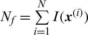is the total number of failure samples, and in this context . It seems that all failure samples are equally contributed to the failure probability estimate. And further, when small failure probability problem is encountered,

In the context of small failure probability, the contribution of a failure sample is approximately reciprocal of the number of failure samples. The meaning of the index can be interpreted as that excluding this point will result in 100/Nf% decreasing in the estimate of failure probability. It also means that when a failure point is obtained, it will result in the increasing of the failure probability estimate by approximately 100/Nf%.

The total contribution of all the failure samples can also be obtained

➁ For another case which the sample falls in the safety region, that is , the index becomes

It can be seen that all the samples in the safety region are equally contributed to the failure probability estimate, which is approximately reciprocal of the number of safety samples.

The total contribution of all the safety samples can also be obtained

Based on Eqs. (8) and (10), it can be concluded that

Comparing case ➀ and ➁, we can obtain that

Eqs. (11) and (12) show the relationship of the contribution indexes for the failure samples and the safety ones. First, they add up to 0, as one of them is positive effect and the other is negative. Second, the contribution of failure sample is nearly 1/Pf times of the one of safety sample in absolute value when small failure probability is encountered. This provides a formal expression and evidence which is consistent with our intuition that failure point should make bigger contribution than safety sample in the estimation of failure probability.

3.1.2 The Contribution of Sample to the Statistical Characteristics of the Estimate of Failure Probability

As it is well-known that, the estimate of failure probability in MCS is unbiased, that is . The variance and c.o.v. of the estimate can be given by

where is the expectation of failure probability estimate.

Substitute (13) into (2) and (14) into (3), then the contribution indexes of sample, e.g., , to the variance and c.o.v. can be derived

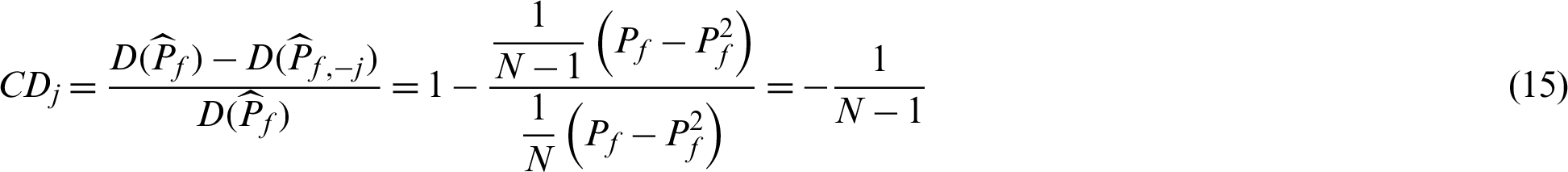
Note that Eqs. (15) and (16) are derived under the condition . It seems that for the variance and c.o.v. of the estimate, all the samples have the same contribution value in a theoretical point of views. This means they contribute equally to the variance or c.o.v. As it is easy to draw that CDj < 0 and , it means that, in theory, adding a new point (no matter what kind the sample is, failure or safety), will result in the improvement of the estimate, e.g., reducing the variance of the estimate by approximate % or reducing the c.o.v. by about %.

However, in the calculation process, the item in the expression of the estimate is usually substituted by the estimate value which is computed by the samples. It is also of practical interest to know how these values actually change. Thus, the practical computed contribution index values are also derived here. First, the variance and c.o.v. are estimated as follows in practical analysis.

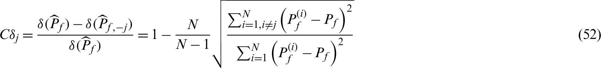
In this context, suppose is a failure sample and if it is taken out, the number of total samples is changed from N to (N −1), and the number of failure samples is changed from Nf to Nf −1, so

In the other case that is safety sample, the number of samples is changed from N to (N −1), and Pf,−j = Nf/(N −1), then the contribution indexes are

It is seen from Eqs. (19) and (21), the computed contribution index values are different for different kinds of samples (safety or failure). However, the corresponding theoretical result in Eq. (15) shows that they are the same for the same kind of sample. The same thing happens to the contribution indexes for the c.o.v.

3.2 Importance Sampling

3.2.1 The Contribution of Sample to the Estimate of Failure Probability

In importance sampling method [6,7], the importance sampling function, , is introduced to compute the failure probability. Suppose a set of samples are generated from , the estimate can be given by:

where is the weighted function used here for simplicity.

In this context, the contribution of a certain sample, , to the failure probability estimate can be derived as:

Similarly, we discuss the calculation of Cj in two different cases as follows.

➀ When , it becomes

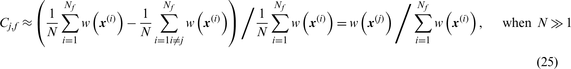
It seems that the failure samples in importance sampling method are not equally contributed to the failure probability estimate comparing to MCS. The contribution of the failure sample is nearly proportional to its weighted function value .

And all the contribution of the failure samples nearly adds up to 1, that is

Especially, for problem with only normal variables, some properties can be obtained. As normal variables can be easily transformed to standard normal ones, we discuss in standard normal space for simplicity. In the standard normal space, the basic random variables is distributed as , the importance sampling density based on the design point can be given by . Suppose a certain number of samples are generated from , the contribution index of sample can be calculated as

where is a constant for a given number of samples. It shows that in this special case, the contribution index is a linear exponent function of the sample value.

In order to see the characteristic of contour line of contribution index, let (a constant value), then according to Eq. (27), we have

where is also a constant value corresponding to . This means that the contour line of the contribution index is linear in two-dimension problem and it is vertical to the design point vector. And in more than 2 dimensions, it is a hyper-plane. It is somehow different from our roughly thought that it may be a circle or hyper-sphere just as the Normal PDF is. In order to illustrate it more clearly, the contour line of the contribution index in the case of two-dimension is shown in Fig. 1.

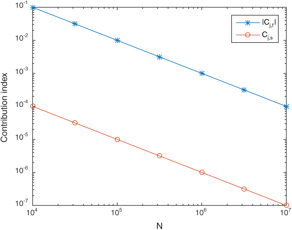
Figure 1: The contour line of the contribution index in the case of two-dimensions

Meanwhile, for points in different contour lines, the values of contribution indexes are exponentially decreasing/increasing, which are shown as

➁ For another case that , it becomes

It can be seen that the expression for contribution index of safety sample is exactly the same as the one in MCS as shown in Eq. (9). However, the values of the number, N, are different when these two methods are applied. This demonstrates the contribution of safety sample in importance sampling is higher than that in MCS as the value of N is usually smaller than that of MCS.

And all the contribution of the safety sample is given by

Thus it seems that

3.2.2 The Contribution of Sample to the Statistical Characteristics of the Estimate of Failure Probability

As well-known that, the estimate of failure probability in importance sampling method is unbiased. The variance and c.o.v. of the estimate can be given by

Similarly, the theoretical contribution indexes of the sample, , to the variance and c.o.v. can be derived

Surprisingly, the expression is exactly the same as those of MCS given in Eqs. (15) and (16). However, as the value of N here is usually smaller than that of MCS, it seems that, generating one more sample in importance sampling method is more effective than MCS in reducing the variance of estimate. This is also consistent with our intuition.

Similarly, in the computational process, all the expectation items in the variance and c.o.v. of the estimate are usually calculated by the samples, i.e.,

Thus, when is a safety sample, the contribution indexes are

And when ,

Finally, the contribution indexes to the variance and c.o.v. can be computed by

3.3 Line Sampling

3.3.1 The Contribution of Sample to the Estimate of Failure Probability

In line sampling simulation [8,9], the failure probability Pf can estimated by:

with the conditional failure probabilities [9,19]

where is the cumulative standard normal distribution function; the limit state function for and ; is the normalized importance direction; is the generated sample set.

The contribution of a certain sample, , on the failure probability estimate can be defined as

Approximately, it can be rewritten as:

It seems that the contribution of sample is proportional to its corresponding failure probability component.

3.3.2 The Contribution of Sample to the Statistical Characteristics of the Estimate of Failure Probability

In line sampling, the estimate of failure probability is also unbiased, and the variance and c.o.v. of the failure probability estimate can be given by

Theoretically,

Similarly, in computational process, Pf is estimated by , and the estimated contribution indexes, and can be easily obtained by using Eqs. (43) and (44).

3.4 Subset Simulation

3.4.1 The Contribution of Sample to the Estimate of Failure Probability

In subset simulation [10], the target failure probability Pf can be estimated by:

where is the generated samples in the i-th level (here i = 0 is corresponding to the whole variable space where Monte Carlo simulation is used); is the indicator function of the (i + 1)-th level; is the estimate of the conditional probability.

For a given set of samples generated in certain level, namely i-th , the contribution of a certain sample, , to the failure probability estimate can be defined as:

Similarly, we still discuss it in two cases, safety sample and failure sample, respectively.

➀ Clearly, the samples in the 1th to th level are all safety samples. In each level, there are conditional failure samples and safety samples.

When and , it represents the case that this sample is generated in i-th level but it does not fall in the (i + 1) level, it is the conditional ‘safety’ sample in i-th level. In this context, the contribution index becomes

When and , it is the conditional failure sample in the (i + 1)-th level, the corresponding contribution index can be

From Eq. (56), it can be seen that the contribution index is not dependent on the target failure probability but the conditional probability and the number of samples used in every conditional level. In practice, the numbers of samples are usually set as the same for the 1-th to -th conditional levels, as well as the conditional failure probabilities, that is, Ni = N and . In this context it can be drawn that the contribution indexes of the conditional failure samples for 1-th to the -th levels are all the same.

➁ when , it is the real failure sample, in this case

For the final m-th level, when Nm = N, hence, either Pm > P0 or may happened, which results in or . This means the contribution indexes of failure samples in final level, which are the real failure samples in target failure region, may be smaller than those in the former levels (1-th to -th levels) which is actually the safety samples.

3.4.2 The Contribution of Sample to the Statistical Characteristics of the Estimate of Failure Probability

The statistical properties of the estimator obtained by Subset Simulation have been discussed in detail in [20]. These results show that the is asymptotically unbiased, and its c.o.v. can be estimated from the Markov chain samples as follows.

First, the variance and c.o.v. of are given by

where

where Ni is the number of samples in the i-th level; is the number of Markov chains in i-th level, and samples have been simulated from each of these chains; Ri(k) is the covariance between and , for any , which is given by

It should be noted that although the ’s are generally correlated, and practical simulation shows that the actual c.o.v. may be well approximated [10] by

And hence the variance can be approximated by

In theory, the contribution indexes can be given by

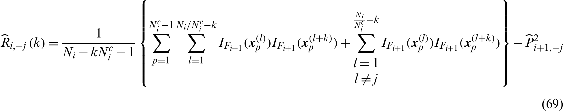
In computational process, Pi+1 is estimated by and is calculated using the Markov chain samples

In order to compute the actual contribution index, suppose the sample, , in the i-th level is taken out of the computation of reliability analysis, then we have

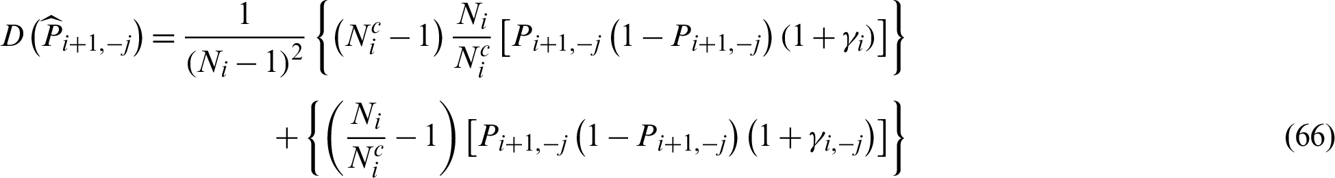
where

Thus the estimated contribution indexes and can be calculated by using Eqs. (43) and (44).

3.5 Summary and Comparison

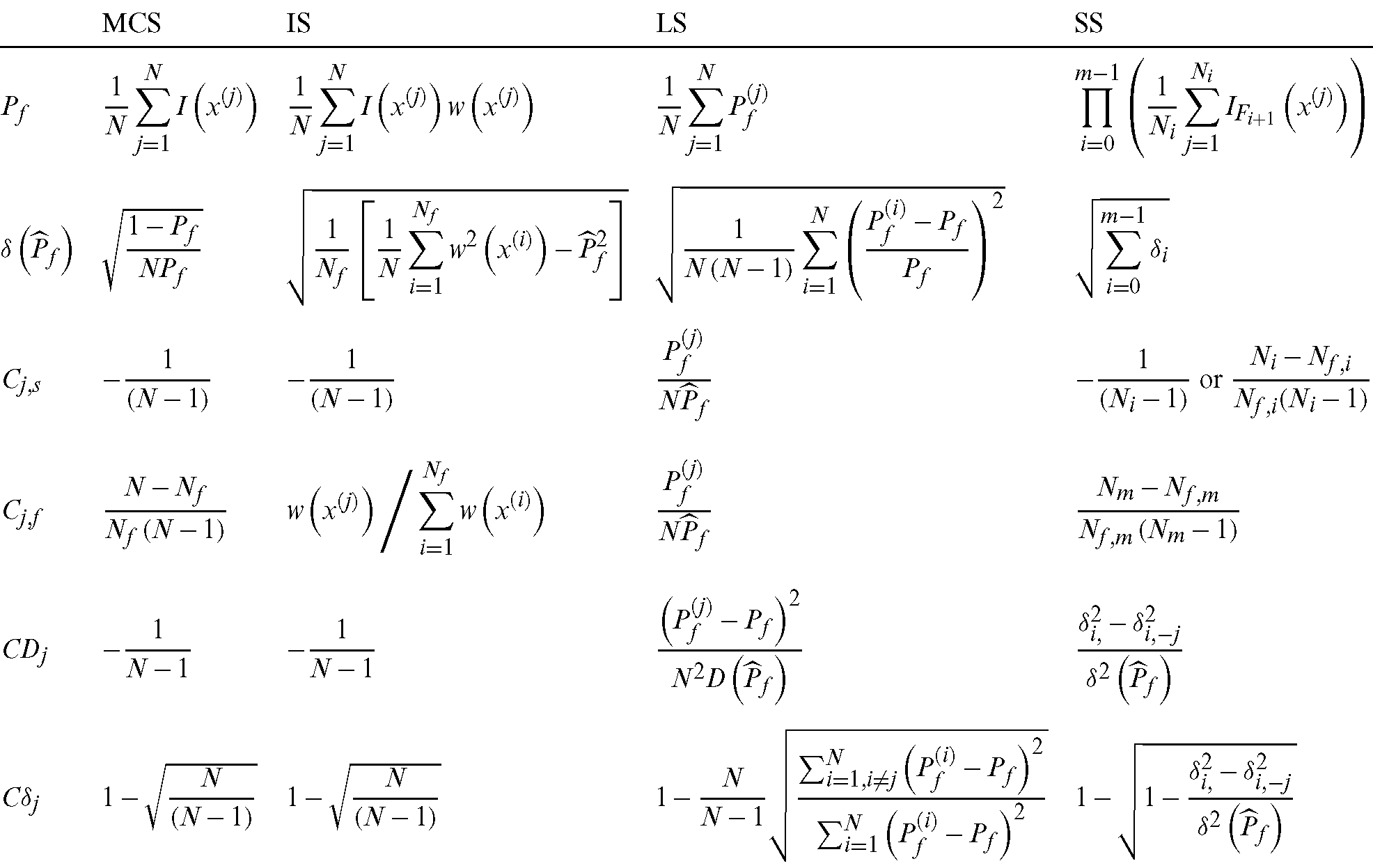
Tab. 1 summarizes in a simplified manner the comparison among the discussed simulation-based reliability methods. As shown in the table, four widely used reliability analysis methods are investigated by using the proposed sample contribution indexes, i.e., Cj, s, Cj, s, CDj and . Among them, Cj, s, and Cj, s quantify the contribution of samples to the failure probability estimate in reliability analysis simulation from two aspect, failure event (sample) and safety event (sample), respectively; while CDj and quantify the contribution of simulated samples to the variance and c.o.v. of the failure probability estimate.

Table 1: Summary of the contribution indexes for different methods

4  Illustrate Examples

Numerical examples are given here to calculate the contribution indexes of the four methods given above. Note that these examples are quite simple reliability problems by themselves, as they are selected to illustrate the findings given above with figures, and the simulation-based method is dependent of the number of dimensions and less affected by the complication of the problem. The first example is a normal linear case that the failure probability is varied from 10−3 to 10−5. The second example is a highly nonlinear case.

4.1 Example 1: Linear Example

The limit state function for the first example, which was also studied in [6], is a n-dimensional hyperplane.

where 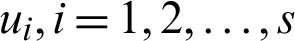are independent standard normal distributed variables. The example was calculated for , and corresponding to s = 2, s = 5 and s = 15, respectively.

The purpose is to investigate the performance of the contribution indexes for different probability levels and different methods.

Tab. 2 shows the computed results for case and s = 2.0 regards the contribution of samples in different methods, i.e., MCS, IS, and SS. As the LS method theoretically only need one sample to compute the failure probability for this linear example, it is not applied in this example.

Table 2: Results of the contribution indexes of different methods for case in example 1

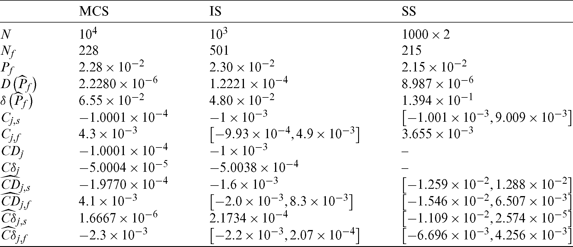
It can be seen from Tab. 2 that in MCS, (1) the contribution index of failure sample is approximately 1/Pf times the one of safety sample; (2) although the theoretical contribution index values of samples to the statistical characteristics are all negative, the computed ones are quite different. For example, and , this means that even the same sample, its contribution to the variance are different from that of c.o.v. According to the result, it shows that missing a failure point will result in the increasing of computed variance but at the same time the decreasing of the computed c.o.v.

For IS method, some findings can also be seen from Tab. 2: (1) The contribution of sample to the failure probability estimate is negative for each safety sample. For failure sample, it varies as the values of sample, for example, within in this example; (2) for both safety and failure samples, the theoretical contribution indexes values to the statistical characteristics are the same with each other, and they are all negative, this means that they are in theory equally contributed to the statistical characteristics; (3) for safety samples the computed contribution indexes to the statistical characteristics and . This means missing a safety point will result in the decreasing of variance but the increasing of the c.o.v.; (4) for failure sample, the computed contribution values to the statistical characteristics are varied as the values of sample, i.e., . Fig. 2 shows the results of contribution computed by IS method for case 1. Only the contribution values of failure samples to the estimate and c.o.v. are shown in the figure. It can be seen from the figure that the contribution index Cj, f is approximately an exponent function from a certain viewpoint in the three-dimension plot, this is also pointed out in Section 3. And it is can be seen that the computed contribution index is not monotonous and has a minimum. This means that different location of samples has different contribution to the c.o.v. of failure probability estimate, even they are all failure samples.

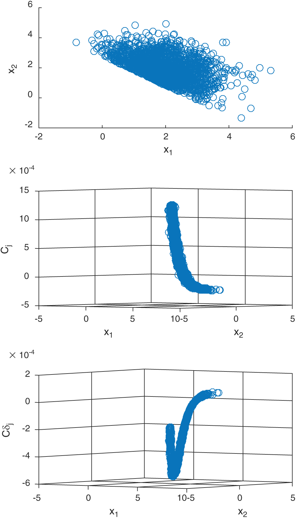
Figure 2: The results of contribution computed by IS method for case 1

For SS method, the following findings can be addressed from Tab. 2: (1) The contribution indexes for all failure samples to the failure probability estimate are positive and equal. For safety sample, it varied as the position of sample in different levels, i.e., within in this example; (2) though the theoretical values of contribution to the statistical characteristics are unavailable, it should be negative form the first principle, as more samples result in more accurate estimate. The performances are some like those of IS method. Note that the values of these indexes are bigger than those of MCS and IS, it means that the samples in SS are more effective in the computation of failure probability. Fig. 3 shows the scatter plot of the contribution results computed by SS method for case 1. It can be seen from the figure that the computed contribution indexes to c.o.v. of the samples in first level are nearly the same, but those of the samples in the second level vary a lot.

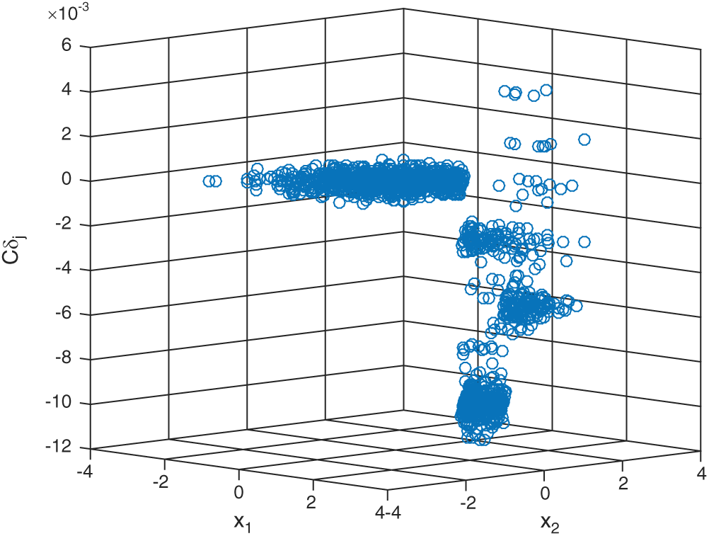
Figure 3: The scatter plot of the contribution results computed by SS method for case 1

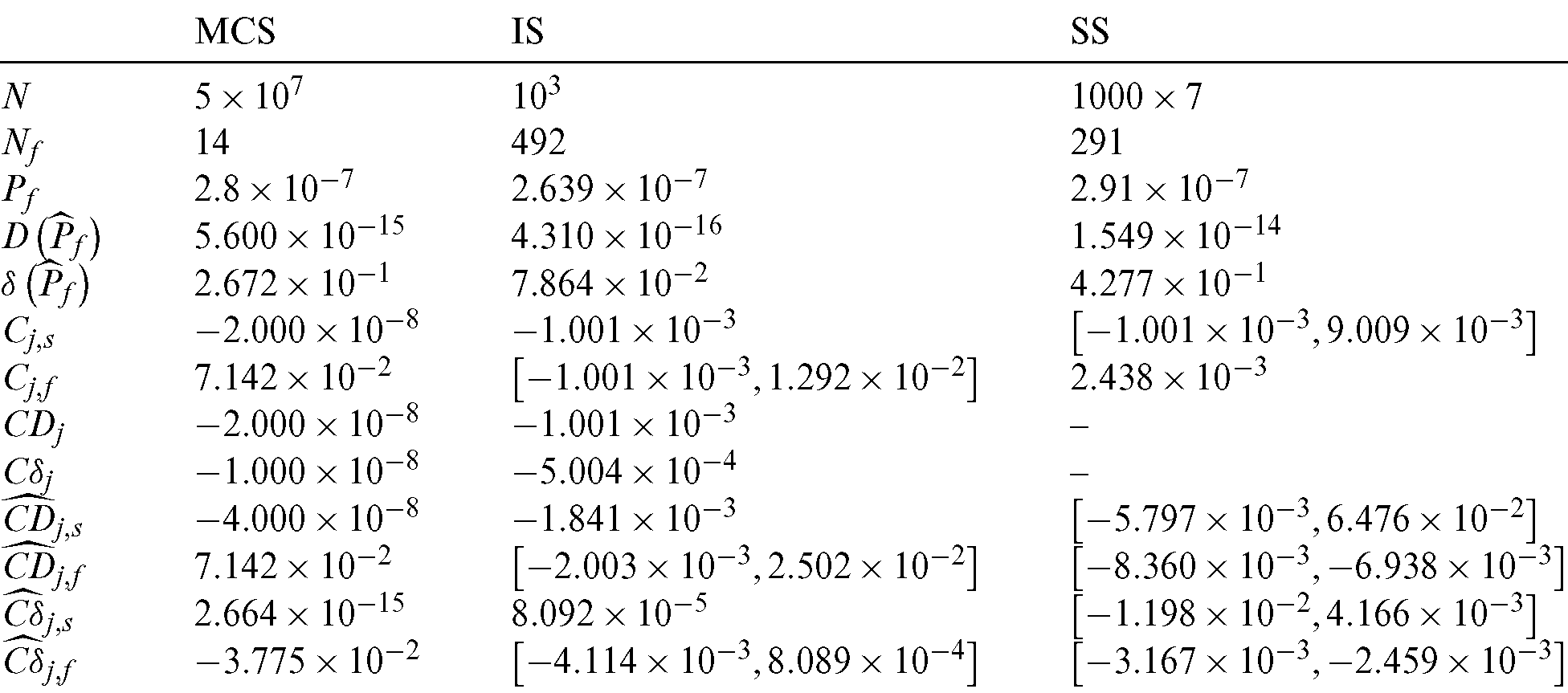
In order to investigate the performance of indexes for different levels of failure probability, Tabs. 2 and 3 show the results for case and , respectively. It seems that the main difference of these methods is the contribution of safety sample. In Tab. 2, when a similar number of failure samples are obtained, the contribution Cj, f values of different methods are approximately in the same order of magnitude, however, the contribution Cj, s values are different from each other considerably. In comparison, the contribution of safety sample of SS method is the biggest in the absolute value among the three methods, and that of MCS method is the smallest. Similar conclusions can be also drawn for the contribution to the statistical characteristics of estimate. This demonstrates that the high efficiency of reliability method is gained from the high contribution of safety sample. For the different levels of failure probability, this becomes more obvious. As in Tabs. 3 and 4, the contribution of safety sample decreases significantly in MCS, while those in IS and SS remain the same level.

Table 3: Results of the contribution for case in example 1

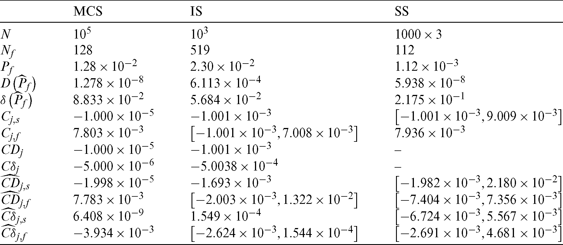
Table 4: Results of the contribution for case in example 1

4.2 Example 2: Nonlinear Example

The limit state function is given by

where x1, and x2 are independent normally distributed random variables, and . This example has been studied by Kaymaz [22].

The contribution indexes of samples of four methods, i.e., MCS, IS, LS and SS, are computed and the results are given in Tab. 5. Note that the contribution indexes of samples in LS method are not divided into safety samples and failure samples. It can be seen that when a total of 500 samples, which is approximately the number of failure samples of other methods, is used in LS method, the corresponding contribution Cj, f values are approximately in the same order of magnitude as those of different methods.

Table 5: Results of the contribution for example 2

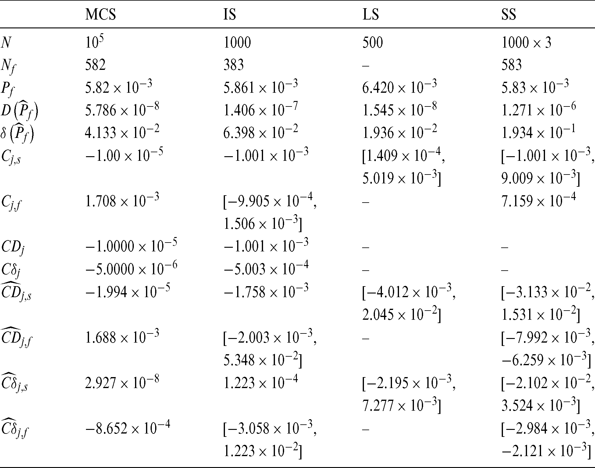
Fig. 4 shows the results of contribution of the sample to estimate, Cj, s, and to c.o.v. of IS method, and also the scatter of the sample is shown in the figure. Still, the contour of Cj, s is exponent, and is not monotonous and has a minimum.

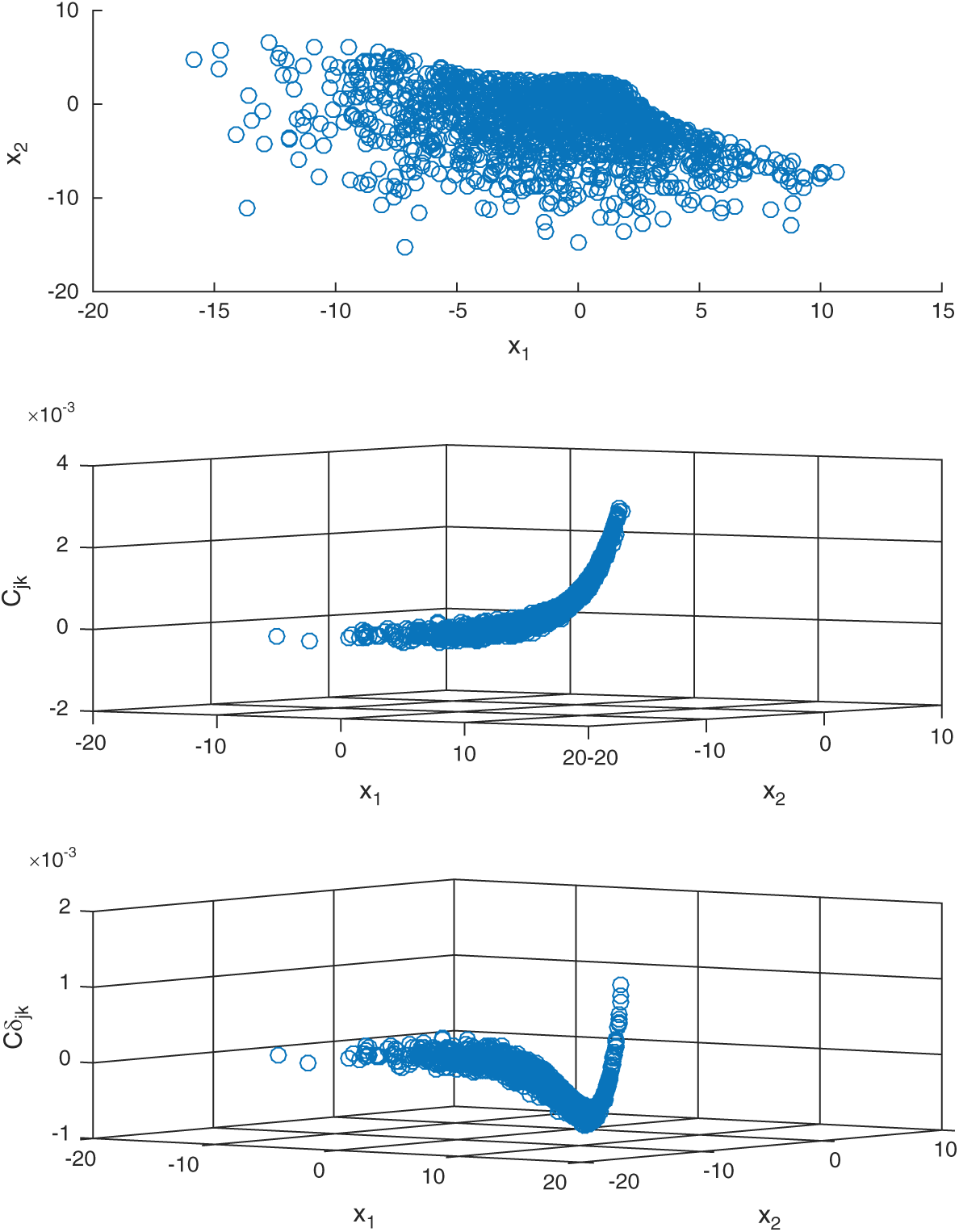
Figure 4: The results of contribution of the sample in example 2

Fig. 5 shows the computed contribution indexes of LS method, as well as the scatter of the samples with the limit state function are shown in the figure. It can be seen that, the contour of Cj in this example is not monotonous, and the contour of is also not monotonous and has more than one minimum.

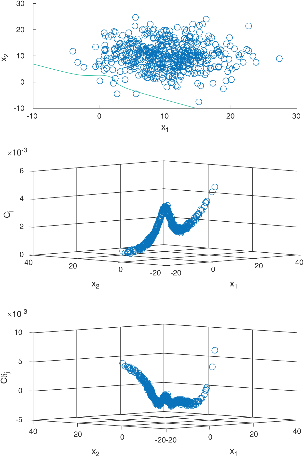
Figure 5: The computed contribution indexes of LS method in example 2

Figs. 6 and 7 show the results of contribution of the sample of SS method. The histogram of Cj, s for the samples in each level is shown in Fig. 6. The left side of the figure shows the results of conditional safety samples in each level and the right side shows the results of failure or conditional failure samples. The scatter plot of all the samples is shown in the Fig. 7. It can be clearly seen that in this example the samples in the second level have the biggest absolute values of contribution index.

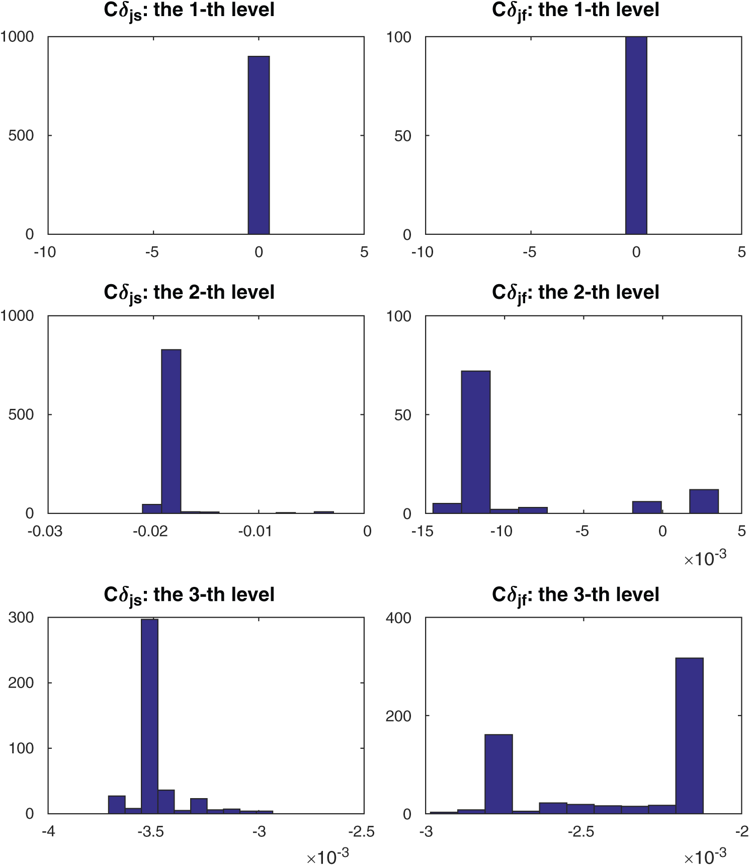
Figure 6: The results of contribution of the sample of SS method in example 2

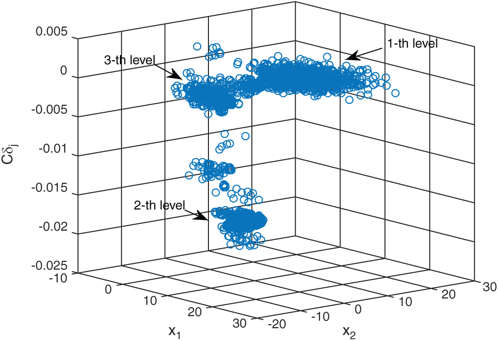
Figure 7: The scatter plot of results of the sample contribution by SS method in example 2

4.3 Example 3: Engineering Example

The reliability of turbine disk is the key to the safety of the aeronautical engine. The fatigue life of an aeronautical engine turbine disk structure (See Fig. 8) is analyzed here.

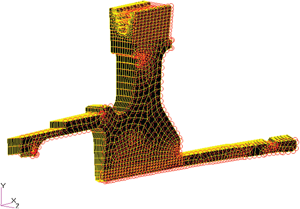
Figure 8: An aeronautical engine turbine disk structure

According to the well-known Mason-Coffin law which is consider the effect of mean stress and mean strain on the fatigue life, the fatigue life can be computed as

where is the fatigue strength coefficient; is the fatigue ductility coefficient; is the mean strain; is the mean stress; b is the fatigue strength exponent of Basquin law; c is the fatigue ductility exponent of Coffin’s law; is the strain range which under 0-takeoff-0 load cycle here; 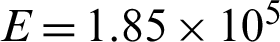MPa is the Young’s modulus.

Considering the actual life under of 0-takeoff-0 load cycle must exceeding the required fatigue life, the limit state function can be expressed as

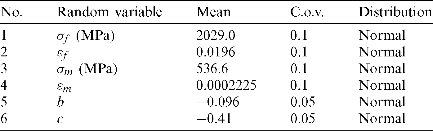
where Nf0 is the required minimum service life and it is set as a const Nf0 = 106 (cyc); Nf is the fatigue life under 0-take-off-0 load cycle computed by Eq. (74). All the random variables are assumed to be normally distributed and the distribution information is given in Tab. 6.

Table 6: The distribution information of the random variables in example 3

The contribution indexes of samples of three methods, i.e., MCS, IS, and LS, are computed and the results are given in Tab. 7. It can be seen that similar conclusions can be made from this engineering case. With approximate same size of failure samples, the contribution Cj in MCS and IS methods are different related to the kind of samples. For safety samples, Cj, f of IS method is about 100 times of the one of MCS, but for failure samples, the contribution indexes, Cj, f, for both of these two methods are in the same order of magnitude. For LS method, Cj varies over a wide range, i.e., from 10−6 to 10−2.

Table 7: Results of the contribution for example 3

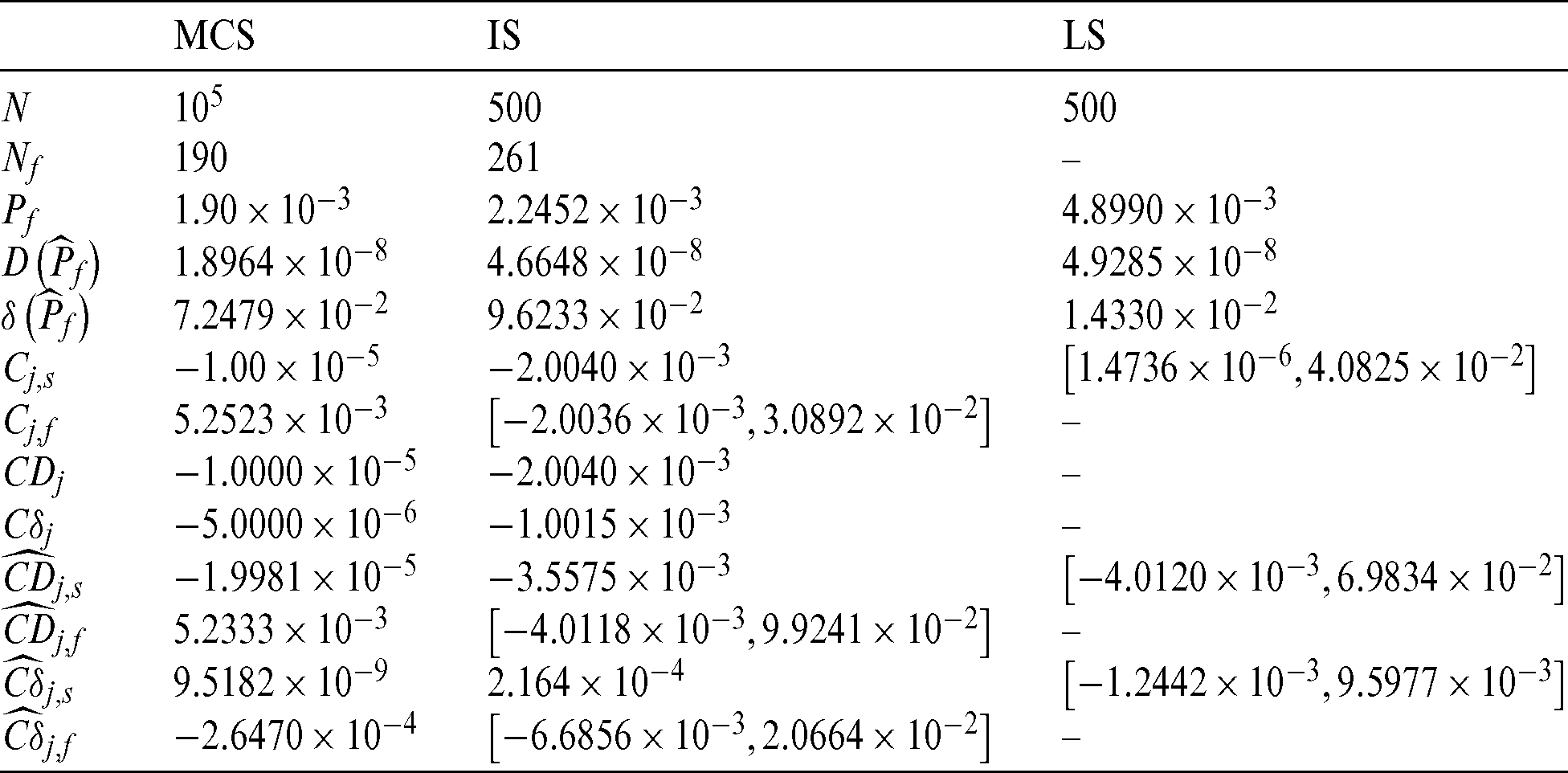
Meanwhile it is found that the contribution and of LS method are nearly in the same order of magnitude with the ones, and of IS method. For safety samples, and of IS method is bigger than those of MCS method inn absolute terms, which is the primary reason IS method is more efficient than MCS.

5  

6  Conclusions

In this paper, three contribution indexes have been proposed, which are the relative changes when a sample is included in reliability calculation or not. The indexes in three simulation-based methods are examined, i.e., Monte Carlo simulation, importance sampling and subset simulation. These indexes are proposed to quantify the sample contribution to the failure probability estimate and its statistical characteristics, thus investigate the efficiency of widely used reliability analysis methods from the contribution of the sample aspect.

Summarizing the arguments, the following findings can be concluded:

1.    For Monte Carlo simulation, results show that the contribution of the failure sample to the estimate is bigger than that of safety sample in failure probability estimation.

2.    For Importance sampling, the contribution index of the failure sample to the estimate is approximately proportional to its weighted function value while the safety samples contribute equally.

3.    For line sampling method, the contribution indexes of the failure sample and safety sample are nearly the same.

4.    For subset simulation, the sample contribution index is related with the conditional probability, but not the target probability to be computed. This can be a good explanation of why SS method owns high efficiency.

The further work should be the implementation of the proposed finding into the active learning in the DoE of surrogate methods, such as the combining of Kriging model with MCS [16], Kriging with IS [17] and Kriging with SS [18,19]. It is noted that the constructed surrogate model may quite sensitive to each selected point, and the most contributed samples are preferred. In this context, the findings and information can be used and incorporated into these methods, further improving the performance. Meanwhile, the proposed indexes may also be used in combination with heuristic algorithm and sampling.

Acknowledgement: The authors would like to acknowledge financial support from NSAF (Grant No. U1530122), the Aeronautical Science Foundation of China (Grant No. ASFC-20170968002) and the Fundamental Research Funds for the Central Universities of China (XMU, 20720180072).

Funding Statement: NSAF (Grant No. U1530122), the Aeronautical Science Foundation of China (Grant No. ASFC-20170968002) and the Fundamental Research Funds for the Central Universities of China (XMU, 20720180072).

Conflicts of Interest: The authors declare that they have no conflicts of interest to report regarding the present study.

This work is licensed under a Creative Commons Attribution 4.0 International License, which permits unrestricted use, distribution, and reproduction in any medium, provided the original work is properly cited.