Computer Modeling in Engineering & Sciences

DOI: 10.32604/cmes.2021.010771

ARTICLE

Fish-Eye Image Distortion Correction Based on Adaptive Partition Fitting

Yibin He1,2, Wenhao Xiong1, Hanxin Chen1,2,*, Yuchen Chen1, Qiaosen Dai1, Panpan Tu1 and Gaorui Hu1

1School of Mechanical and Electrical Engineering, Wuhan Institute of Technology, Wuhan, 430205, China
2Hubei Provincial Key Laboratory of Chemical Equipment, Intensification and Intrinsic Safety, Wuhan, 430205, China
*Corresponding Author: Hanxin Chen. Email: *pg01074075@163.com
Received: 28 March 2020; Accepted: 18 May 2020

1  Introduction

The fish-eye lens is widely used in security monitoring and intelligent transportation because of its short focal length, wide viewing angle and wealth of picture information. However, due to its short focal length, the image acquired by the fish-eye camera is distorted [1–6]. This distortion makes it difficult for people to obtain useful image information [7–12].

There are many ways to deal with this distortion. Zhang et al. [13] proposed an algorithm for correcting fish-eye lens image distortion that is based on circular segmentation. The algorithm uses the coordinate transformation of the circle and the circumscribed square to divide the circular fish-eye image into concentric circles. Then, the corresponding circumscribed squares are found. After that, each pixel of the fish-eye image is corrected to the corresponding pixel of the square edge to complete the correction. However, this method is only suitable for circular fish-eye images, and the correction effect is not ideal. There is a significant stretching effect in the diagonal region, and the deformation of the original image is more pronounced, especially in the central region of the image. The traditional latitude and longitude mapping fish-eye image correction method, which was first proposed by Kum et al. [14] and improved by Yang et al. [15], is more consistent with the conventional visual habits of humans. The basic idea of the latitude- and longitude-based fish-eye image correction method is to project the points of the fish-eye image into the corresponding latitude and longitude coordinate system. The mapping process is similar to the mapping of the Earth’s plane map. First, each point of the image is mapped to the sphere, which is located in the latitude and longitude coordinate system. Then the points on each meridian have the same abscissa value according to the distribution of latitude and longitude. The larger the value of longitude, the greater the distortion. The points on each latitude have the same ordinate value. However, for the upper and lower parts of the fish-eye image, the image has been significantly stretched and distorted due to a certain overcorrection of the original image. Wei et al. [16–19] indicated the fish-eye image correction method based on polynomial fitting. The method corrects the image taken by the same fish-eye lens with an improved correction effect. In this method, the fish-eye image is first divided into regions. Then the coefficient of the polynomial equation is determined and the fish-eye image is corrected through the use of the polynomial fitting method. However, the correction effect is not ideal for all lenses, and a certain amount of information is still missing in the diagonal direction of the image.

This study proposes an adaptive partition fitting method to correct fish-eye images. This method uses the same basic concept as the polynomial fitting method, but improves upon its applicability. To solve the problem of different cameras having different distortion coefficients, we determined that the center point and the relative position of the corner point are unchanged by comparing the different image distortion regions with the original image. Thus, a quantitative corner point can be selected in the image. Because the calibration plate background is simple, this study adopts an improved fast method to find the corner point. Taking each pixel as the center, the four adjacent areas of pixels were investigated. If the values of all pixels in the neighborhood are 0, the pixel is an angular point. The distortion degree can be expressed according to the change in distance from the corner point to the center point before and after the distortion. The selected corner points are classified by this value. The corner points whose distortion difference is smaller than a specific threshold value are classified into one type. The region where these points are located is defined as a distortion area. As a result, the image is partitioned by this method. Finally, the model is built and the region is corrected by fitting the function. The present study verifies the practicability of the method through three sets of experiments.

2  Principle of Distortion Generation and Correction

2.1 Text Layout

The fish-eye lens has a short focal length and a viewing angle close or equal to 180. The focal length can generally reach 16 mm. The special fish-eye lens focal length will be shorter, resulting in the fish-eye lens being a super-wide-angle special lens [20,21]. Thus, except for the center of the picture, other scenes that should be horizontal or vertical have changed accordingly. Fig. 1 shows the structure of the Canon EF 15 mm f/2.8 fish-eye lens, and Fig. 2 shows the image taken by it.

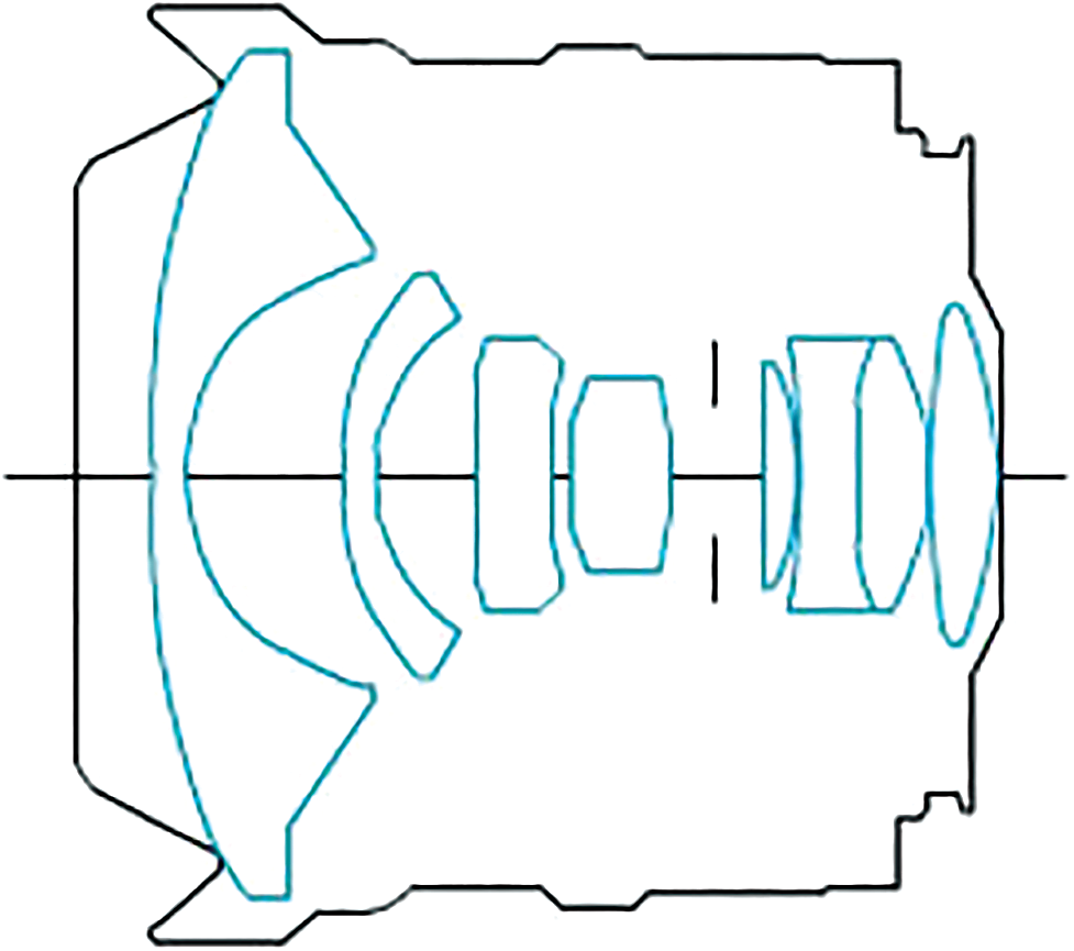
Figure 1: Structure of Canon EF 15 mm f/2.8 fish-eye lens

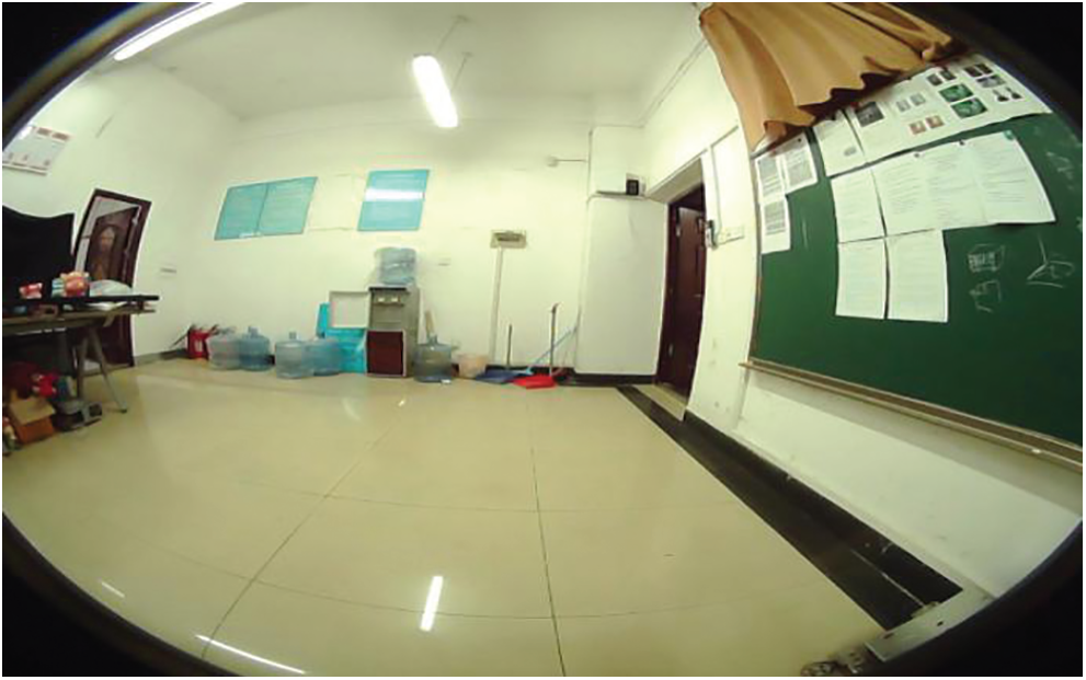
Figure 2: Image taken with fish-eye lens

Because of the different structure of the fish-eye lens, the images taken by it are very different from the ones taken by an ordinary camera. An ordinary camera follows the principle of similar imaging, but the imaging of fish-eye lenses is primarily non-similar imaging. In similar images, the image and the object are different in size, and the virtual image direction is opposite to the object. However, the fish-eye lens imaging process involves four coordinate systems: The global coordinate system, the camera coordinate system, the imaging plane coordinate system and image coordinate system [22], as shown in Fig. 3.

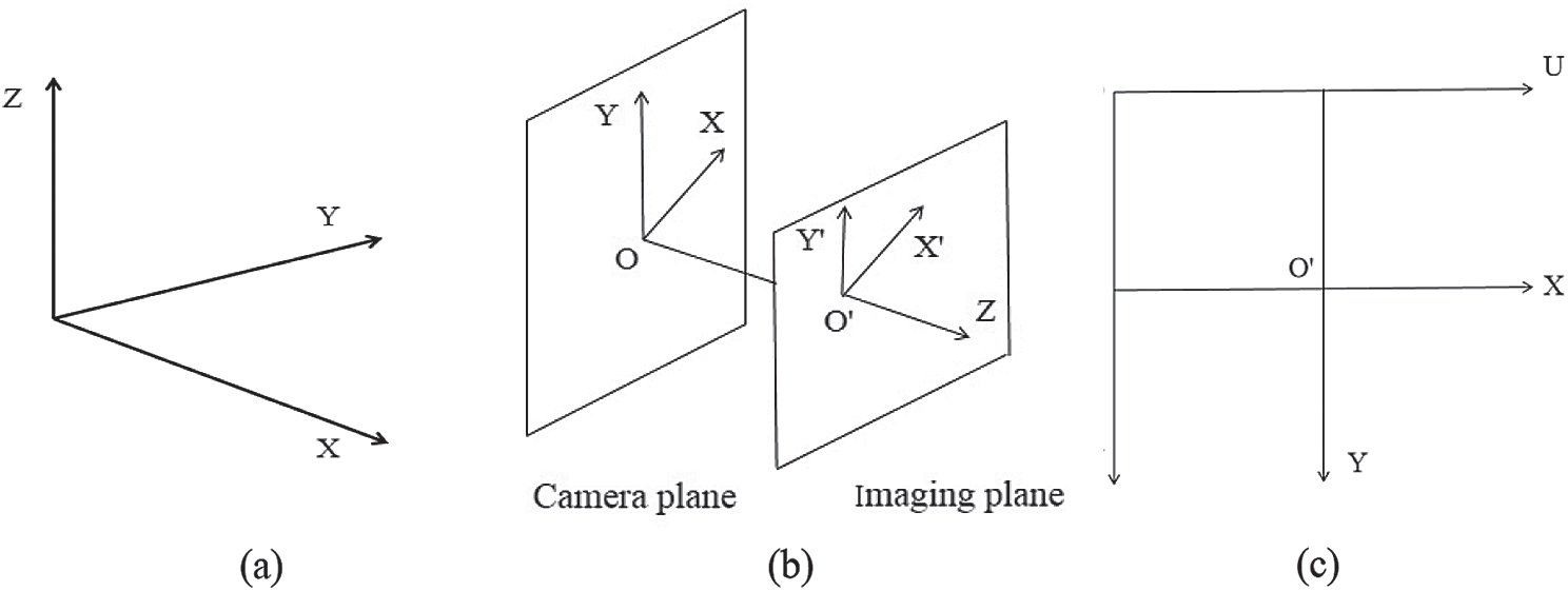
Figure 3: Coordinate systems. (a) Spatial coordinate system, (b) The camera coordinate system and the imaging plane coordinate system, (c) Imaging plane coordinate system

The world coordinate system is used to describe the coordinate information of the object in real space. It is a 3D coordinate system. The global coordinate obeys the right-hand rule. The global coordinate system can determine the real position of points on the image plane. The global coordinate system is shown in Fig. 3a.

The camera coordinate system is the coordinate system established for the lens, which is also a 3D coordinate system. The origin is at the optical center of the camera. The X-axis and Y-axis are parallel to the imaging plane, the direction of the Z-axis is along the camera optical axis, and the XYZ axes conform to the right-hand rule. The distance from the origin of the camera coordinate system to the imaging plane is the focal length, as shown in Fig. 3b.

The imaging plane coordinate system is a 2D coordinate system established by the photosensitive array for imaging inside the camera. The intersection point between the lens optical axis and the photosensitive array is the origin O. The X-axis and Y-axis are parallel to the X-axis and Y-axis, respectively, in the camera coordinate system. Fig. 3b shows the camera coordinate system and the imaging plane coordinate system.

The image (pixel plane) coordinate system is the coordinate system established for the 2D image plane generated by camera acquisition. The origin of the image coordinate system is set at the upper left corner of the image. The X-axis and Y-axis are parallel to the X-axis and Y-axis of the imaging plane, respectively. As shown in Fig. 3c, UOV is the image coordinate system, and O′ is the image center, where the unit of image plane is in pixels, and the unit of imaging plane is in mm.

The fish-eye lens is regarded as a hemispherical model [23–27], as shown in Fig. 4. Let the point locate at A(x, y, z) in the global coordinate system, and the point projected to the camera coordinate system is A1(x1, y1, z1). Through the light refracted by the fish-eye lens, the imaging point of the projection point on the imaging plane is A2(x2, y2), and the imaging point in the image coordinate system is A3(u, v). A1 is the image of A in the lens, which is refracted to A2 through the lens.

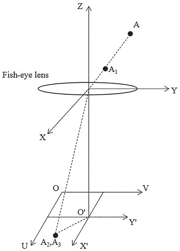
Figure 4: Process of fish-eye lens imaging

(1) Global coordinates to camera coordinates

Point A is transformed linearly from the world coordinate system to the camera coordinate system. It is given by the rotation matrix R and a translation vector T:

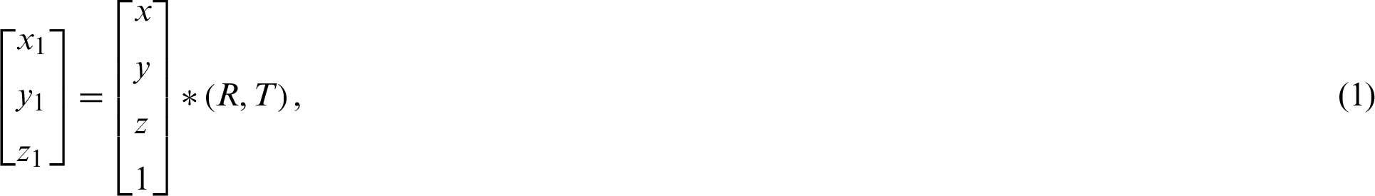
where the rotation matrix R is expressed as

Translation vector T is expressed as

where R and T describe the parameters of the external scene of the camera.

(2) Camera coordinates to imaging plane coordinates

The light from point A goes through the fish-eye lens, and, through the refraction of multiple sets of lenses, the light path changes. The resulting image will have a certain deviation in the the photosensitive array imaging plane, and the deviation process is nonlinear.

Taylor’s formula is frequently used to represent a general model of the projection pattern of a fish-eye lens. The transformation relation between the camera coordinate system and the imaging plane coordinate system can be expressed by formula (4):

(3) Image plane to image coordinate system

The coordinate system established on the imaging plane is expressed in mm. The resulting image is expressed in pixels. The two coordinate systems have different origin positions. According to the imaging plane coordinate system and the image coordinate system, a simple coordinate transformation can be carried out to obtain the transformation relation, which is shown in formula (7):

where c, d and e are the radiative transformation coefficients, and u0 and v0 are the image center.

If the height of the object is y, the lateral magnification is , the ideal height is y′, f is the focal length of the object, and is the half angle of view of the object side. The relationship between them can be described by formulas (8) and (9).

The distance between the object and the lens is finite:

The distance between the object and the lens is infinite:

It can be determined from formulas (8) and (9) that if , the ideal height will be negative, and the result is not true. The view angle of the fish-eye lens is greater than or equal to . At this time, the fish-eye lens imaging analysis cannot use the traditional similar imaging principle. A more suitable mapping relationship should be chosen to represent the correlation between objects and images. The common models for fish-eye image analysis are as follows.

1.    Isometric projection: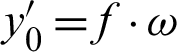

2.    Stereoscopic projection: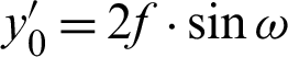

3.    Stereoscopic projection: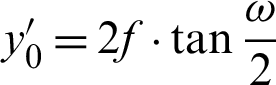

4.    Orthogonal projection: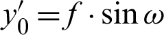

The fish-eye image formation formula curve is shown in Fig. 5.

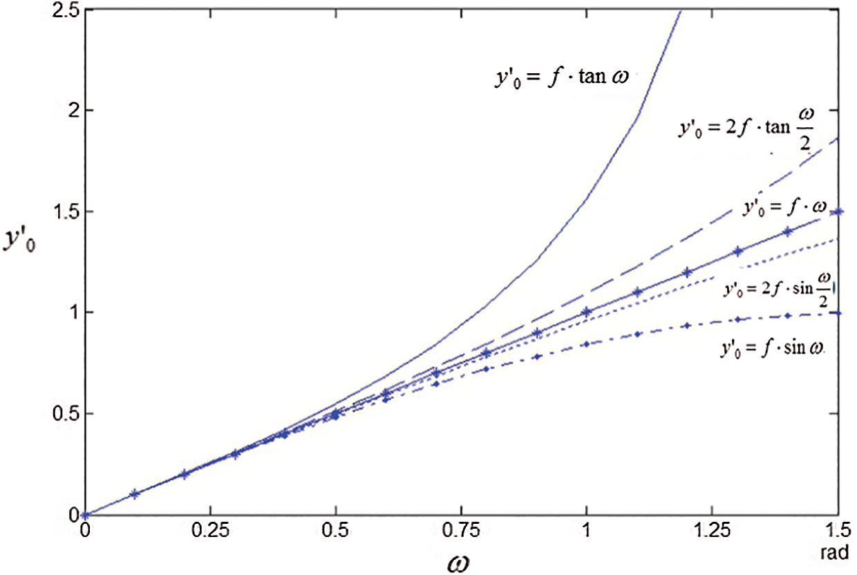
Figure 5: Fish-eye image formation model curve

Fig. 5 shows the distortion curve of fish-eye lens drawn according to the above model. The difference between the curve and curve reflects the deformation of each model. Because the distortion degree is only related to the path of the light, no matter how the image is distorted, the distortion will change the shape, information, and corner position of the image. However, the relationship between image sharpness and image-to-one mapping does not change. That is, once the imaging formula is determined, the relationship between the images does not change regardless of how the image is distorted. Because the equidistant projections have equal radial distances on the phase plane in the same field of view, the imaging height is proportional to the object’s viewing angle. The required information can now be easily derived, and it is highly precise and in real-time. For this reason, this imaging thought model is now widely used.

2.2 Principle of Malformation Correction

Fig. 6 shows a schematic diagram of the optical imaging principle [28,29] of the ordinary lens and the fish-eye lens.

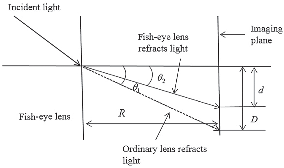
Figure 6: Schematic diagram of the distortion of the fish-eye lens

In Fig. 6, is the angle between the incident light and the optical axis, is the theoretical refraction angle after the object enters the lens, is the actual refraction angle of the object after entering the fish-eye lens through the incident light, D is the distance from the theoretical image to the optical axis, d is the distance from the actual fish-eye image to the optical axis, n is the refractive index, and R is the distance between the lens and the imaging surface. The following formulas can be obtained:

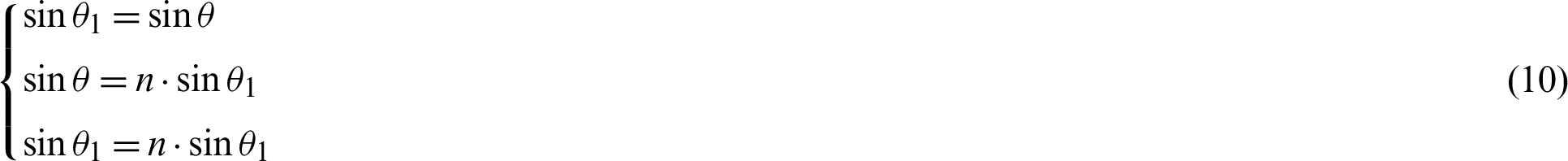
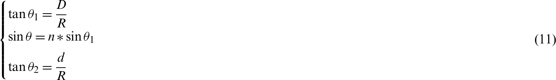
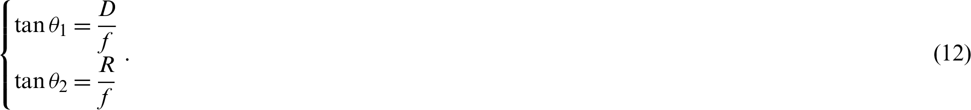
The relation between R and D can be deduced from formulas (12) and (14) as follows:

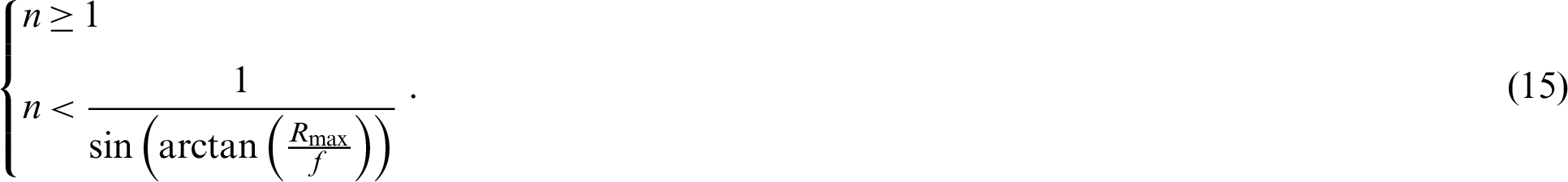
The value of n is a parameter determined by the actual lens. According to the requirements of the definition domain of trigonometric function and the definition of refractive index, the value range of n can be calculated:

In the image taken by the fish-eye lens, the central area remains unchanged, and the noncentral area is distorted. The fish-eye image can be corrected to be a normal image, as long as the function relation between and “d” and “D” is found. The image can be corrected to an image that matches the normal viewing angle of the human eye.

3  Adaptive Partition Fitting

3.1 Principle of Adaptive Partition Fitting

The principle of traditional correction fitting algorithm is to coordinate the fish-eye image under the premise of the known fitting polynomial. The size of the traditional image is obtained by polynomial fitting, and the polynomial is used to calculate the position of the original image point in the corrected image. The pixel filling is carried out finally in [9], but this method does not have good adaptability. For different fish-eye pictures taken by different fish-eye lenses, the same polynomial cannot obtain good results. Moreover, since the image is not uniformly distorted, the degree of distortion in the various regions is different. Therefore, if the same formula is used to express the distortion for different areas, the image information will be lost. To better illustrate this theory, the following experiments are carried out in this paper. Fig. 7a shows a segmented image composed of discrete points, whose segmentation relation satisfies the following equation:

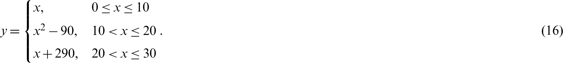
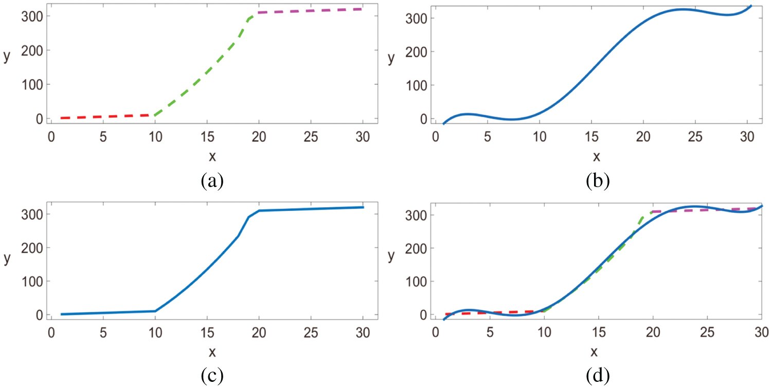
Figure 7: (a) Piecewise function. (b) Fitting function of the fifth-order polynomial. (c) Piecewise fitting function of the fifth-order polynomial and (d) comparison diagram

By fitting this group of discrete points with a polynomial function, experiments show that the fifth-order polynomial can contain the discrete points as possible, as shown in Fig. 7b. If each segment of the fifth-order polynomial is fitted, the effect of Fig. 7c will be obtained. Fig. 7d shows the difference between piecewise fitting and direct fitting. Obviously, if a single polynomial is used to fit all discrete points, it cannot truly reflect the real situation of piecewise function.

According to the fish-eye image imaging effect, the distortion that is closer to the center of the fish-eye image is smaller, and the distortion closer to the edge is larger, so the fitted curve shape should meet the following points.

1.    Pass through the origin (0,0);

2.    Be a continuous differentiable curve;

3.    When r is small, r changes slowly; when r is large, r changes quickly;

4.    The curve increases monotonously;

5.    The curve order is as low as possible to reduce the computational complexity.

According to the above conditions, it can be concluded that the curve fitted by the fifth-order polynomial is the most in line with the requirements, so this paper uses the fifth-order polynomial to correct the fish-eye image.

This method presented in this study conducts a reverse correction of each fish-eye lens, which is similar to the camera calibration principle. By using the imaging principle described in Section 2.1, the distances from the pre-correction and post-correction corner points to the center are found first. No matter how distorted the image, the object-to-image mapping relationship is unchanged. Therefore, the corner points are the first selected to be recorded in the checkerboard. However, because there are few corners, this is not a good reflection of the real situation. Therefore, we need to select more feature points for calculation. Accordingly, this paper connects the corner points with each other. The intersection point of the line connecting each corner point is also regarded as the feature point. In this cycle, a sufficient number of feature points can be obtained for correction. The principle is shown in Fig. 8.

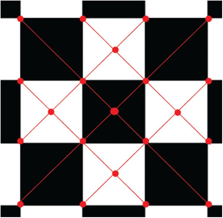
Figure 8: Diagram of checkerboard pattern. The red line is the corner line and the red point is the feature point

Then, according to the polynomial in formula (18), the mapping relationship between “d” and “D”, which is suitable for the fish-eye lens, can be fitted:

The difference between “d” and “D” reflects the degree of distortion at that point. The larger the difference, the deeper the degree of distortion. The difference is set as the distortion difference of the point (m is the serial number of the point in the figure). A threshold value “T” can be set by this principle. If the difference between points in a region of the graph is less than or equal to “T”, then the distortions at these points are similar. Thus, these points can be classified into one class. Then, using the polynomial to fit each class and complete the correction:

If h < T , points m and k are in the same area. Then, formula (14) is applied to this kind of fish-eye camera image to implement subarea fitting and complete the correction. It can be seen from Fig. 8 that the horizontal and vertical pixel values are all 0 in the eight areas of the corner pixel. Therefore, if the horizontal and vertical pixel values are close to 0 in the eight areas of the corner pixel, the point is the corner point.

3.2 Implementation Steps of Adaptive Partitioning

The proposed algorithm’s implementation steps are as follows.

1.    Find as many corners as possible, as shown in Fig. 9b. The upper right corner is numbered as the first point, and the points are numbered sequentially, as shown by the black dots in Figs. 9a and 9b;

2.    Find the values of d , D , and jm corresponding to each point in the two pictures;

3.    Find the value of h of point 1 and other points, and set a threshold of T. If h < T , then classify this point with point 1 as a group until all the same class points as point 1 are found. Name all the points in this group (initial number is 0). The first point is where h > T is named point 1 again. Cycle Step (3), and let N (Number of the distortion regions, each time the grouping process is completed, the value is increased by 1) add 1.

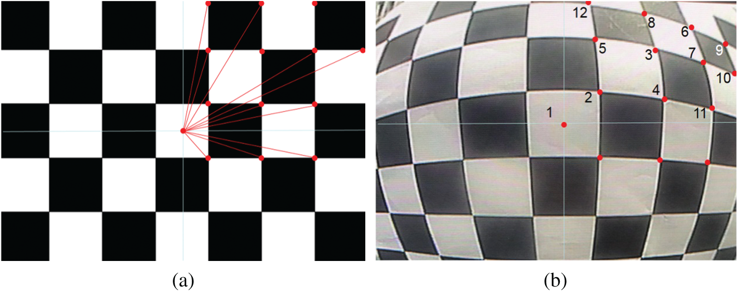
Figure 9: Ordinary lens checkerboard image. (a) Fish-eye checkerboard image. (b) Red dots are the corners

Using Fig. 9 as an example, the results are shown in Tab. 1. The algorithm threshold is set to 25. Start with the midpoint of the image. The points numbered 1, 2, 3, 4, 5, and 11 are the first group. The points numbered 7, 8, and 12 are the second group. The points numbered 6, 9, and 10 are the third group.

Table 1: Comparison of distortion value

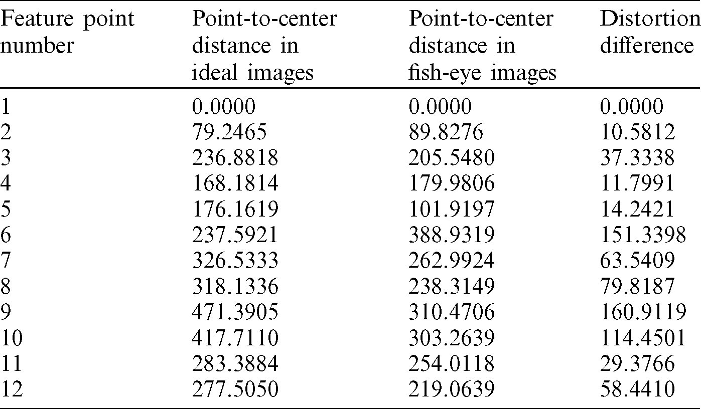
All points in the area after automatic partitioning in Step (3) are fitted by formula (5), and the polynomial corresponding to the fish-eye lens in each area is obtained. As can be seen from Tab. 1, the fitted polynomial curve is a piecewise curve. Starting from the origin (0, 0), the first segment of the curve has the gentlest curvature, the third segment has the largest curvature, and the second segment has a small curvature. The algorithm flow chart is shown in Fig. 10:

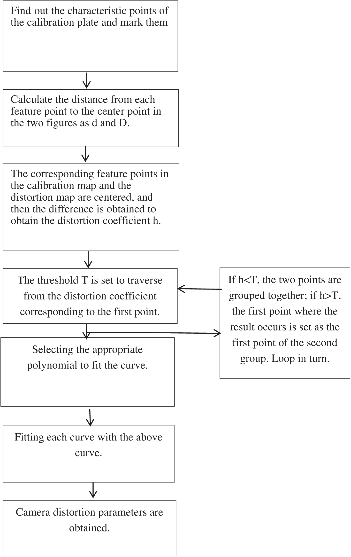
Figure 10: Algorithm flow chart

Each point in the picture obtained under the fish-eye lens is partitioned according to Step (3). Then these areas are fitted by the polynomial obtained in Step (4). The corrected position of each point is then obtained, and the correction process is completed.

4  Experimental Results

In the experiments conducted for this study, three sets of pictures were selected under the same fish-eye lens. The results obtained by using the latitude graph correction method and the adaptive partition correction method were then compared. The algorithm was compiled and implemented in MATLAB 2014. The five correction steps were

1.    Select feature points on the regular picture in checkerboard format and the picture taken with a fish-eye lens. Extend the line between the corner point and the midpoint, and the intersections with the image can be regarded as feature points. If a large number of feature points are needed, the intersection points can also be connected, thereby obtaining more feature points. The more feature points selected, the more accurate the result, as shown in Figs. 6a and 6b;

2.    Calculate the distortion value and difference of each point in the two graphs;

3.    Partition with adaptive partitioning algorithm;

4.    Fit the data in each region by using polynomials. The result is shown in Fig. 11;

5.    Complete the correction.

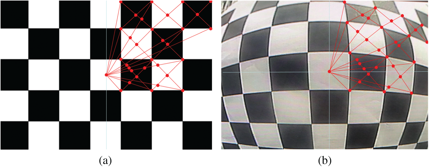
Figure 11: Ordinary lens checkerboard image. (a) Fish-eye checkerboard image. (b) Red points are the intersection of the corner point and the line connecting the corner point

This paper selected 40 feature points, as shown in Fig. 11b. The third-order, fourth-order, and fifth-order images were used for comparison. The polynomial that best matched the point dispersion law was selected, and the subarea was then partition fitted. The shape obtained after fitting achieved the effect of a distortion fish-eye image. The fitting results are shown in Fig. 12. The abscissa X is the distance from the feature point in the standard image to the center of the image, and the ordinate Y is the distance from the feature point in the fish-eye image to the center of the image.

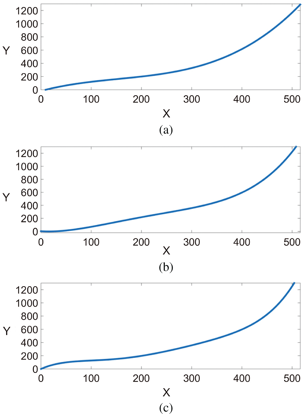
Figure 12: Various order polynomial fitting effect diagrams. (a) Third-order polynomial fitting curve. (b) Fourth-order polynomial fitting curve. (c) Fifth-order polynomial fitting curve. The abscissa X is the distance from the feature point in the standard image to the center of the image, and the ordinate Y is the distance from the feature point in the fish-eye image to the center of the image

According to the principle set forth in Section 3.3, the fifth-order polynomial of Fig. 12b is the most suitable for formation of fish-eye images. For this reason, the fifth-order polynomial was selected as the reference point. The subarea was then partition fitted. The first point of each group was the segmentation point. There were three groups in total with two segmentation points, and each segment was fitted by a fifth-order polynomial. In this experiment, adaptive partitioning divided the points selected in the graph into three regions. The correction effect is shown in Fig. 13 (the continuous curve is a fifth-order polynomial, and the segmentation curve is a curve for each region). The pictures that were taken under the fish-eye lens were divided into regions by the abscissa of the segmentation points, and all the points in the region were fitted by using the corresponding fifth-order polynomial to achieve the fitting effect. The more feature points obtained, the more explicit the partition, and the more accurate the correction effect. Because the third part was badly distorted and the point coordinates oscillated, the last part did not obtain a smooth curve.

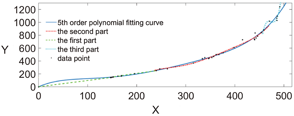
Figure 13: Segmentation fit diagram

Fig. 14 contains four fish-eye shots. The corresponding pictures are corrected with the method in this paper.

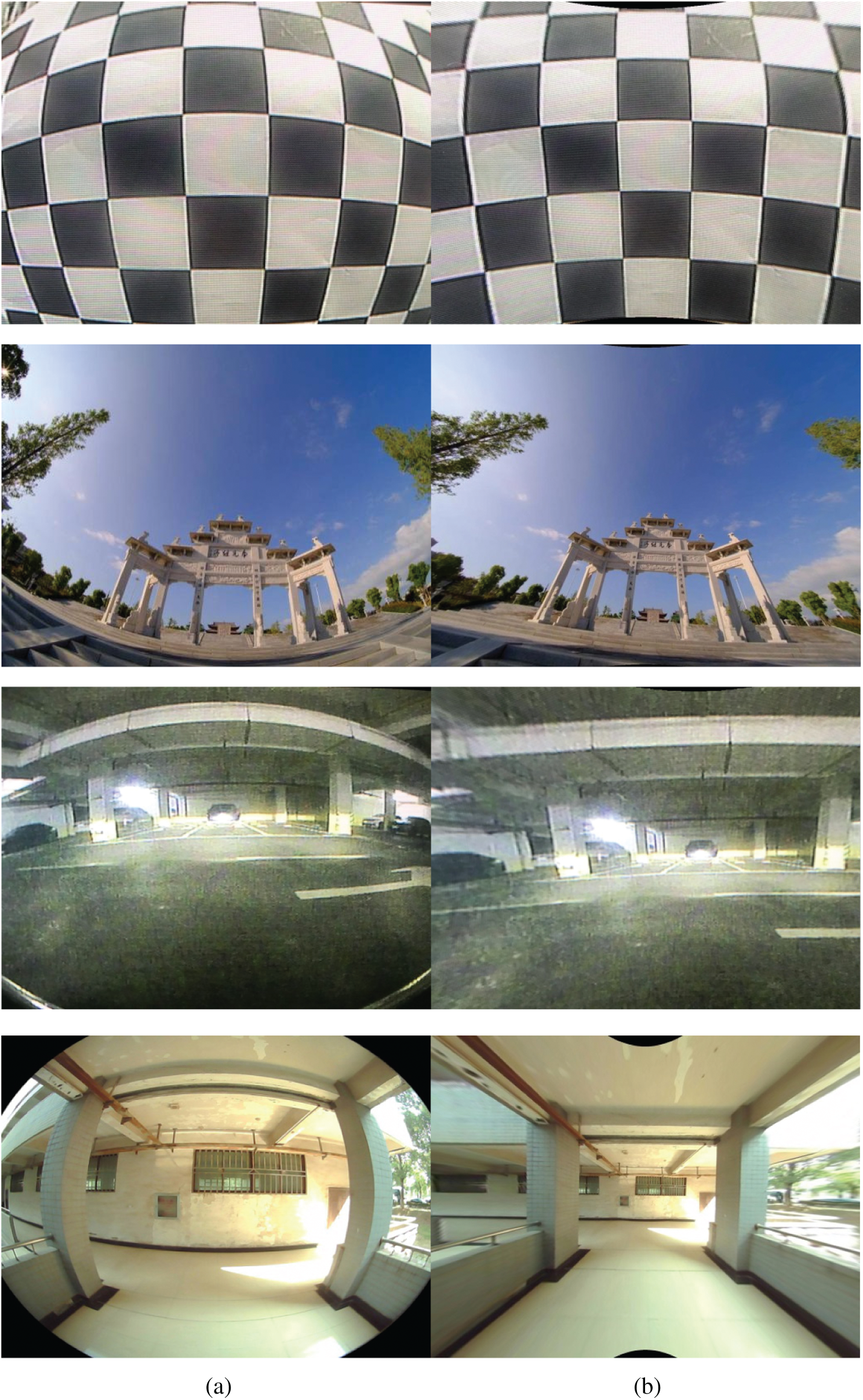
Figure 14: Comparixsson of effects of the partition fitting correction and traditional correction algorithm. (a) Original image. (b) Partition fit correction image

It can be clearly seen from Fig. 14 that the partition fitting correction method can be used to inversely fit the difference of the distortion degree in each region. This method obtains better results than the conventional method.

5  Conclusions

According to the imaging characteristics and correction principle of fish-eye images, a method of fish-eye image correction based on adaptive partition fitting is proposed. The method begins with the original undistorted picture. The images taken by different lenses are next connected in reverse order. Then adaptive partitions are formed according to the difference of the distortion degree of the feature points in the image. Finally, the polynomial that is most suitable for the image correction is determined. The correction method covers a wide area and does not cause information loss in the image. The effectiveness and practicability of the method are proved by experiments.

Funding Statement: This work was supported by the National Natural Science Foundation of China (Grant No. 51775390) and the Open Research Fund Program of Hubei Provincial Key Laboratory of Chemical Equipment Intensification and Intrinsic Safety (Grant Nos. 2016KA02 and 2018KA01).

Conflicts of Interest: The authors declare that they have no conflicts of interest to report regarding this research paper.

This work is licensed under a Creative Commons Attribution 4.0 International License, which permits unrestricted use, distribution, and reproduction in any medium, provided the original work is properly cited.