Computer Modeling in Engineering & Sciences

DOI: 10.32604/cmes.2021.011823

ARTICLE

Fracture Reactivation Modeling in a Depleted Reservoir

Mengtao Cao1,2, Weiguo Liang1,2, Shunde Yin3,*and Maurice B. Dusseault4

1College of Mining Engineering, Taiyuan University of Technology, Taiyuan, 030024, China
2Key Laboratory of In Situ Modified Mining of Ministry Education, Taiyuan University of Technology, Taiyuan, 030024, China
3Department of Civil and Environmental Engineering, University of Waterloo, Waterloo, N2L 3G1, Canada
4Department of Earth and Environmental Sciences, University of Waterloo, Waterloo, N2L 3G1, Canada
*Corresponding Author: Shunde Yin. Email: shunde.yin@uwaterloo.ca
Received: 01 June 2020; Accepted: 21 September 2020

1  Introduction

Reservoir permeability enhancement through injection-based hydraulic fracturing is widely studied for improved oil production and shale gas development as well as coal bed methane (CBM) and other unconventional oil and gas recovery [1–4]. Less attention is paid to natural fracture reactivation induced during oil and gas production processes and its implication on reservoir permeability, despite its relatively common occurrence [5] During production, an oil or gas reservoir shrinks (V) as the effective stresses increase. The shrinkage is impeded laterally by the “infinite” earth, but there is far less vertical constraint from the overburden, which will subside somewhat in response to reservoir shrinkage. Based on linear elastic assumptions, the total horizontal stresses in the reservoir will decline significantly during depletion, whereas the total vertical stress decreases only marginally, but with some local redistribution leading to effects such as increased vertical compression near the flanks of the reservoirs. Based on a poroelastic behavior [6], as pore pressure declines uniformly in a reservoir, the vertical effective stresses increase significantly, whereas the horizontal effective stresses increase substantially less (about 1/3 as much for a laterally extensive, flat-lying geometry [7]. Based on the Coulomb friction criterion [8], the increasing deviation in the effective vertical and horizontal stresses (i.e., increasing deviatoric stress or shear stress) may reactivate existing natural fractures and cause fracture slip, depending on the strength and orientation of the fractures, and their initial stress conditions. This problem can be addressed in the context of contact mechanics.

The contact problem, an issue central to solid mechanics, refers to the stress, strain and damage phenomena that take place when two solid surfaces interact [9]. Contact problems have widespread applications in geomechanics, and one embodiment is natural fractures subjected to changing stresses, leading to processes such as pre-existing fault rupture, joint or bedding-plane surface slip, and dilative opening of new and existing fissures because of slip. These are all associated with the relative dislocation (shear slip) of the discontinuity (contact) between two surfaces and include the basic concept of Coulomb frictional slip between opposing contacting surfaces [10,11]. Contact surfaces that slip with respect to each other are viewed as Mode II and Mode III cracks within the formalism of engineering fracture mechanics: Mode II is co-directional slip (crack propagation direction coincident with activating shear force direction); Mode III is anti-directional slip (crack propagation direction at a large angle away from the direction of the principal activating shear force–-sometimes called “tearing”). In the contact problem, the shearing force along the crack face is vital for calculating the stress intensity factor (SIF), the direction and rate of crack propagation, and has a significant influence on the deformation, strength and stability of the structure of cracked media [12–14].

A challenge to the analysis of contact-slip problems using conventional finite element methods lies in the need to adequately remesh the domain during crack nucleation and propagation, including the use of extremely fine meshes and issues of mesh-dependency of crack propagation. To help overcome these challenges, the extended finite element method (XFEM) is used to model cracks with arbitrary geometric shapes within the framework of FEM approaches based on the Partition of Unity method; this enriches the standard FEM approximations by using additional discontinuous interpolations near the propagation crack tips [15]. Unlike FEM, XFEM does not require mesh topology updating; instead, the interpolation functions between the finite element mesh and the discontinuity are mathematically “enriched” [13,16–20].

XFEM is widely applied to solve crack problems in reservoir engineering, including branched and intersecting faults [15,18,21,22], cohesive crack propagation [23–25], and 3-D thermal crack propagation [26,27]. The contact problem is a highly nonlinear constrained problem, so generally, it can be solved using XFEM with both primal and dual formulations. Khoei et al. [28] and Liu et al. [29,30] employed a conventional penalty method to model frictional contact with XFEM, which has also been extended to large deformation contact problems [31].

In this article, the XFEM and frictional contact model are employed to simulate the behavior of rock discontinuities in producing reservoirs. In the numerical experiments, we analyze the effect of Young’s modulus, the crack orientation, and the frictional coefficient of the crack surface on the distribution of stress and displacement after some reservoir depletion.

2  The Framework of Frictional Contact Problems Using XFEM

2.1 Contact Problem Modeling

The constitutive model for contact friction must be stipulated before numerical modeling of the contact problem because it provides the physical description of the contact mechanism between the two bodies. Assuming two bodies, a slave and a master body denoted by and , respectively (Fig. 1), the relative displacement from the point S to the point M is expressed as

where and denote the displacement vectors of master point M and slave point S, respectively. The relative displacement can be decomposed into normal and tangential gap displacements expressed as follows:

where is the unit vector normal to the surface of the master body, and and are the identity tensor and projection tensor, respectively.

Figure 1: A contact between two bodies

If the two parts of the surface are in contact, there will be traction along the contact surfaces. The contact surfaces can be defined by the standard Kuhn–Tucker relations [29]:

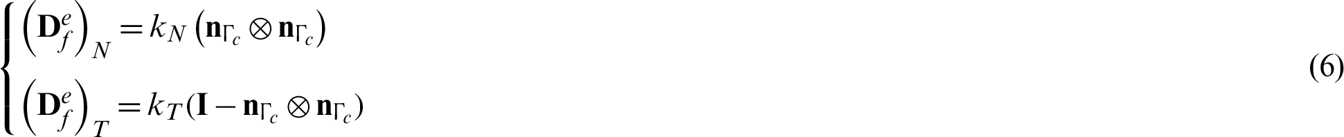
In this study, the penalty method is selected to cope with the contact constraints, and the penalty parameters kN and kT represent the normal and tangential stiffness constants on the contact surface, respectively. For the contact surfaces, the constitutive law can be written as

where and are the normal and tangential stresses on the contact surface, and and are the tangential and normal parts of the elastic matrix for contact friction, which can be expressed by

A stick-slip criterion is needed to determine whether the contact surface is in a state of adhesion or slip, and the most widely used is Coulomb’s friction law [14]. In two-dimensional states, the shear surface changes to a line, and the Mohr–Coulomb frictional yield function in the one-dimensional state is

where cf is the unit cohesion, and f is the frictional coefficient of the contact surface. Eq. (7) can be rewritten as

The “stick” condition applies if the magnitude of the right side is greater than that of the left side; in contrast, “slip” arises if the magnitude of the right side is less than the left side. If slip along the surface takes place, the tangential tractions need to be recalculated and returned to the magnitude of the right side to achieve a static, non-slipping state.

2.2 Modeling Frictional Contact with XFEM

The general equations of contact problems using XFEM are needed, and the situation is sketched in Fig. 2. Consider a domain with a discontinuity which divides the domain into two bodies, the slave () and master () bodies. The displacement boundary condition is applied on the external boundary , the stress () boundary condition 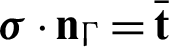is applied on the external boundary , and the contact boundary condition is applied on the contact boundary . For the contact problem, the final weak form of the equilibrium equation can be obtained as [32].

where is the virtual displacement field and pc is the contact stress vector along the contact surface. To model the discontinuity of the contact interface, enriched new degrees of freedom are introduced by the Heaviside function H(x) to the nodes related to the discontinuity. For an enriched element, the XFEM displacement approximation function u(x) can be written as:

where N and Nenr denote the set of all nodal points and the set of enriched nodal points in the domain, respectively. denotes the standard nodal degree of freedom, and is the enriched nodal degree of freedom. In addition, and are the standard shape functions with H(x) being the Heaviside function. The displacement value at the node according to Eq. (10) is not equal to the node displacement, and the corresponding displacement approximation can be written in order to make the displacement value at the node equal to the nodal displacement by translating the enriched function as

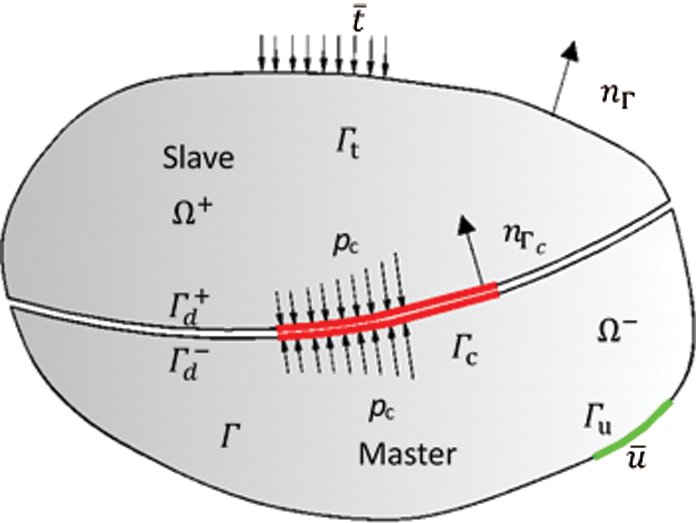
Figure 2: Definition of a contact problem

The Heaviside function is given by:

where is the level set function, which is the signed distance function that can be defined as

in which denotes the closest point to the point x on the contact surface, with being the vector normal to the contact surface at the point . Therefore, the displacement jump on the contact surface can be given by

Based on the relationship between the strain vector and the approximate displacement, the corresponding strain vector (x) can be obtained as follows

where involves the spatial derivatives of the enriched shape functions and contains the spatial derivatives of the standard shape function. Here, L denotes the matrix differential operators defined as

2.3 Modeling of Contact Constraints Using XFEM

Various modeling techniques are employed to introduce the contact constraints stipulated in Section 2.2 into the weak form of the FEM equation for the contact problem, such as the penalty method [32–34], the Lagrange multipliers method [35–37], and the augmented-Lagrange multipliers method [22]. Herein, the penalty method is chosen to derive the frictional contact constraint formulation. For the penalty method, the normal contact force is related to the “penetration distance” between the two bodies by using the normal contact stiffness, and the tangential contact force is calculated by the tangential contact stiffness and the tangential slip between the two bodies. For the sake of deriving the XFEM solution for the contact problem, the displacement and stress fields , , are substituted into Eqs. (11), (14) and (15), then into the weak form of the equilibrium equation (9), and the equilibrium equations can be written as follows, based on the minimum total potential energy principle

Rearranging the integral equilibrium equation, and it can be written as

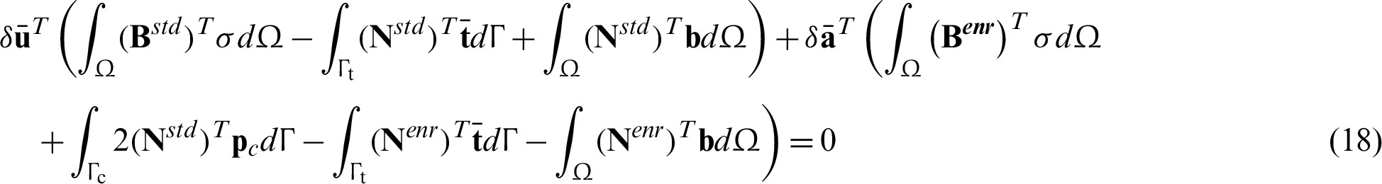
According to the Eq. (18), the following sets of equations can be obtained

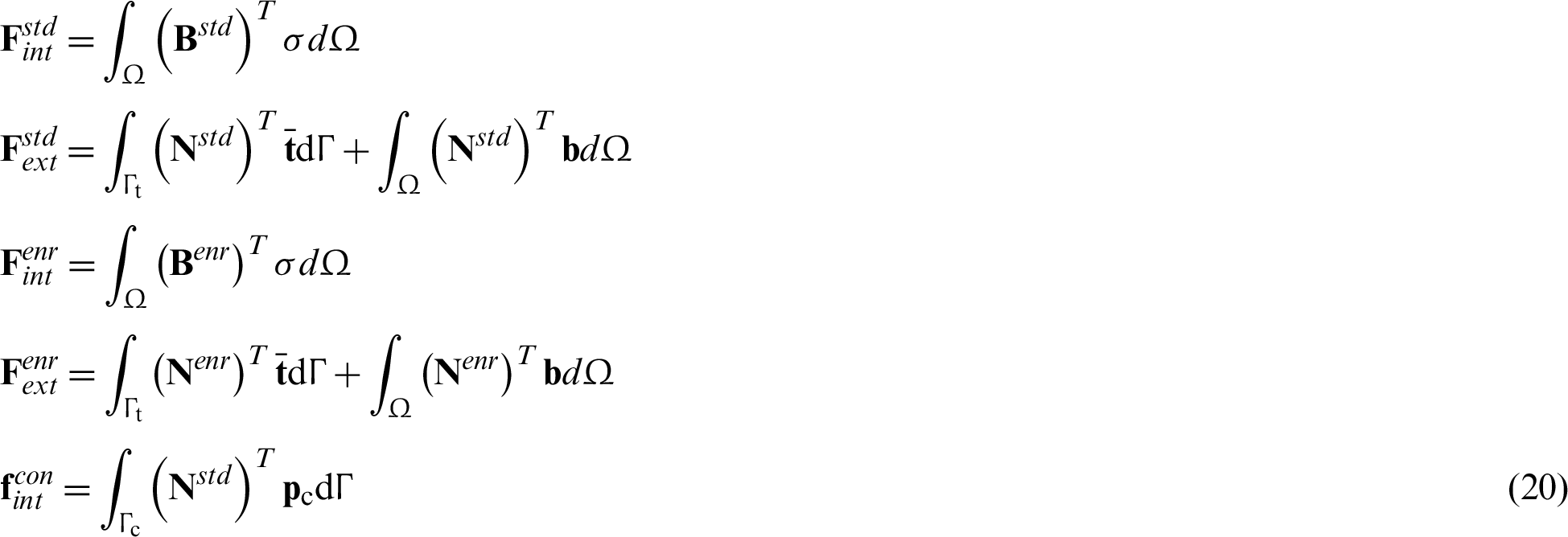
where F matrices are associated with the weak form of the XFEM equation, i.e., Eq. (9), as

The Newton–Raphson iterative procedure [38] is chosen to linearize the discretized governing equations, and a first-order truncated Taylor series is employed to expand the residual equations, so the linearized equations for iteration i + 1 of time interval (n, n + 1) can be written as

where and denote the increments of the standard and enriched nodal displacements at iteration i + 1 of time interval (n, n + 1), respectively. The stiffness matrices K are

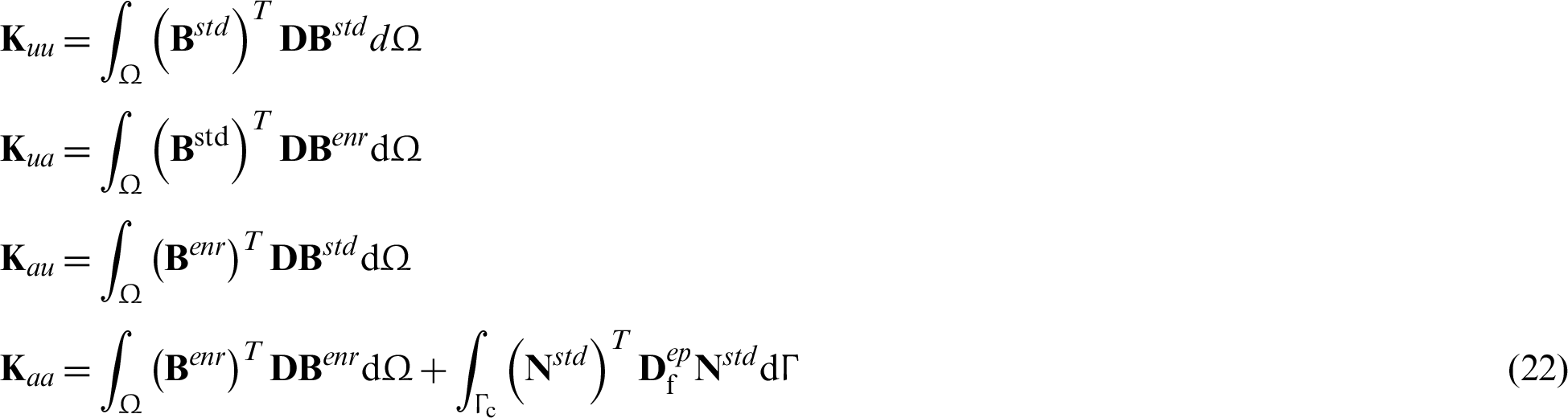
In which denotes the continuum tangent matrix for the contact problem [18], which can be defined as

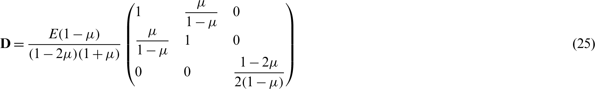
D is the elastic matrix and for the plane stress case,

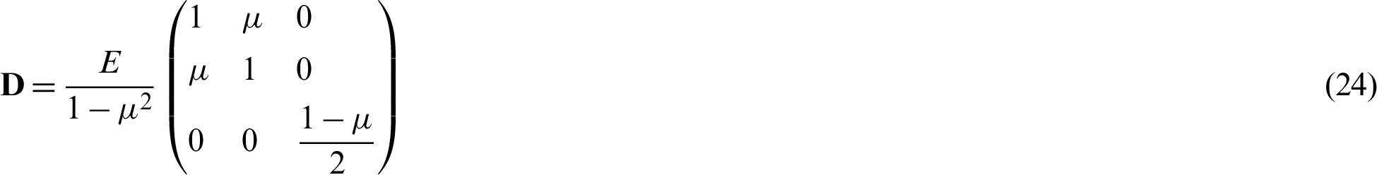
whereas for the plane strain case,

The return mapping algorithm is central to the numerical solution of plasticity problems, taking much of the computational time [22]. Frictional contact problems and slip are plasticity problems, and a similar return mapping algorithm is used to solve the contact stresses on the contact surface. The normal and tangential contact stresses and can be calculated iteratively. In this paper, the penalty parameters are initially set to several orders of magnitude greater than that of Young’s modulus E of the material, 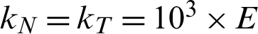. Assuming that the tangential contact stresses at iteration n and the new Gauss point displacements on the contact surface at iteration n are given, the tangential and normal contact stresses at iteration n + 1 are

where is the increment between tangential displacement in iteration n and n + 1. Then, this equation is used to check the tangential contact force at iteration n + 1.

If the equation is not satisfied, then both the tangential contact force and the tangential penalty parameter are updated using the following correction

The residual force vector can be used to evaluate solution convergence by , with being the prescribed target percentage error.

3  Verification

In this section, the frictional contact codes developed here are verified using an elastic plate with an oblique fracture [29]. The plate is m with a 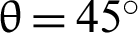inclined crack, and the top edge is subjected to a uniform vertical displacement , whereas the bottom edge is fixed. The geometry model is discretized with 2601 nodes and 2500 four-node isoparametric elements. The material is elastic with Young’s modulus and Poisson’s ratio . The contact constraints are applied using the penalty method with the parameters N/m3, and the fracture has a parameter f = 0.1 as the frictional behavior.

Fig. 3 displays the deformed XFEM mesh; it shows a tangential relative displacement across the contact interface. Fig. 4 presents the comparative contours of horizontal and vertical displacement fields [29]. The results show that our solutions are almost the same as those of Liu et al. [29], a reasonable validation.

Figure 3: The deformed XFEM mesh for the elastic plate

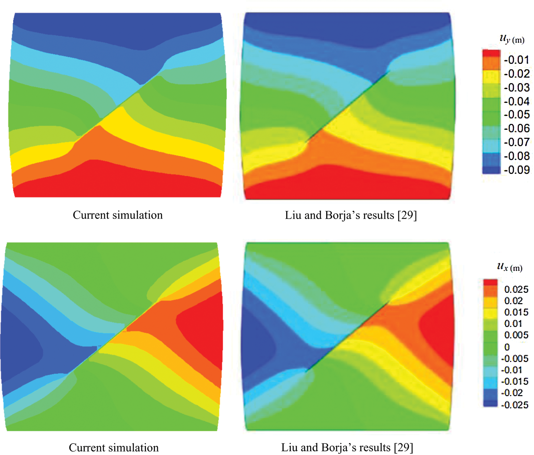
Figure 4: Horizontal and vertical displacement field contours for the elastic plate

4  Numerical Example

During oil and gas production, the pore pressure drawdown changes the stress state in the reservoir and surrounding strata, which may cause fault reactivation, slip of natural fractures and bedding planes, and alteration of reservoir permeability by fracture dilation, especially in the case of fracture-flow dominated reservoirs. We focus on the issue of a single fracture slip arising from a stipulated depletion. Assume a depleted reservoir with the vertical maximum principal stress and the horizontal minimum principal stress , with a central 0.6 m long fracture inclined at (Fig. 5). The lower boundary is a zero vertical displacement condition with horizontal displacement permitted. The fracture is allowed to have tangential movement but the fracture tips do not propagate. We use a 2D plane-strain model with Young’s modulus of 5 GPa and Poisson’s ratio of 0.3; the contact constraints are applied with the normal penalty parameter N/m3 and the tangential stiffness N/m3. The fracture has a friction coefficient of f = 0.1.

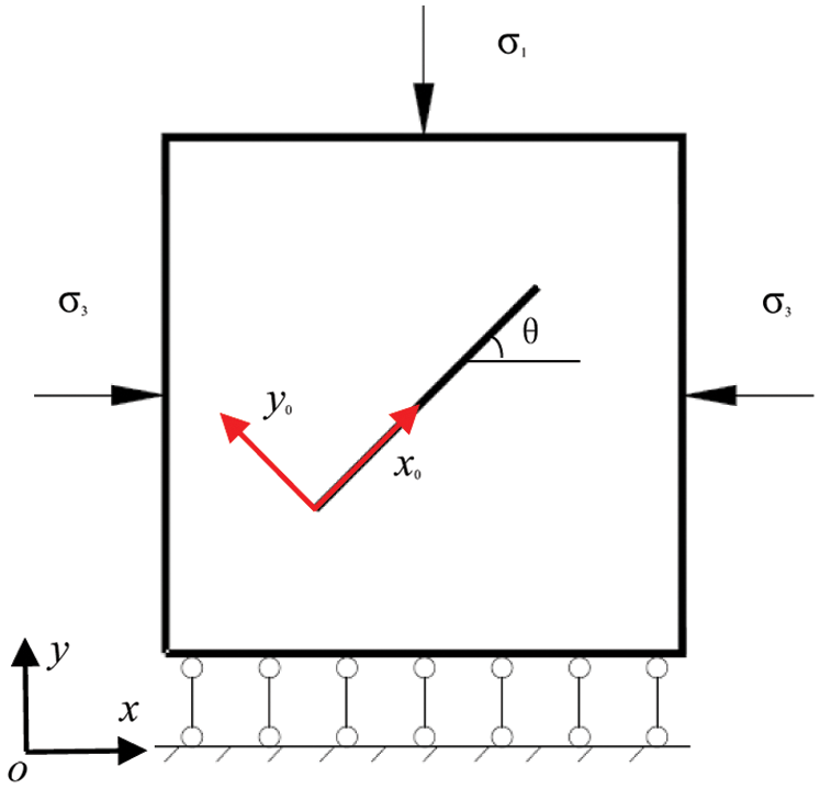
Figure 5: Geometry and boundary conditions

4.1 The Effect of Young’s Modulus

To investigate the effect of Young’s modulus on the distribution of displacements and stresses around the fracture, simulations are performed on the same XFEM mesh and physical parameters but with three different Young’s moduli, 5 GPa, 20 GPa, and 80 GPa respectively.

Figs. 6 and 7 illustrate the horizontal and vertical displacement fields for three different Young’s moduli; there exists an obvious displacement discontinuity across the fracture, and tangential movement along the interface occurs under deviatoric compressive stresses. With increasing Young’s modulus, both horizontal and vertical displacements decrease, and the possibility of tangential movement along the contact plane drops as well.

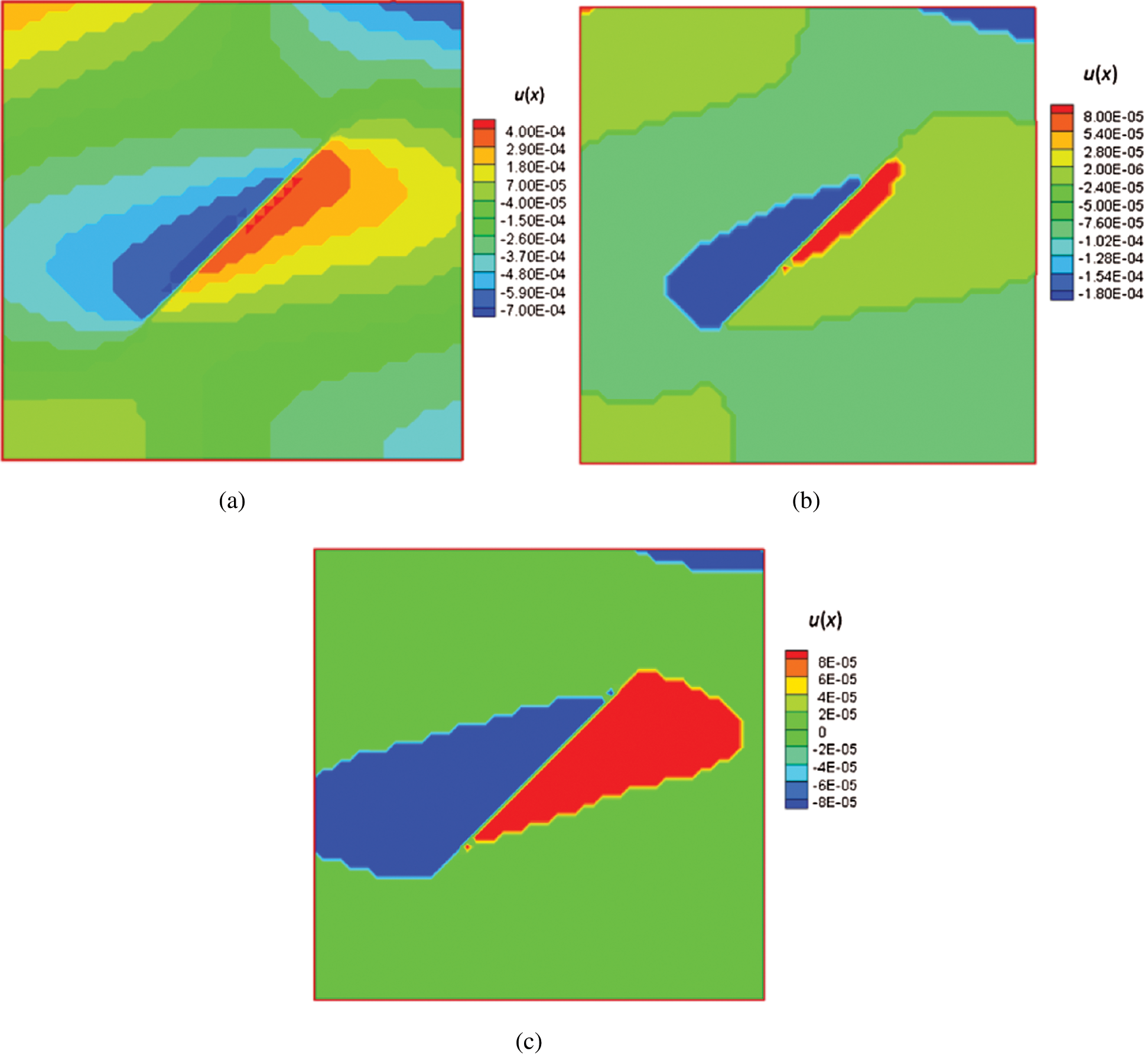
Figure 6: Contours of horizontal displacement of the elastic plate with different Young’s moduli (color bar in units of meters). (a) E = 5 GPa. (b) E = 20 GPa. (c) E = 80 GPa

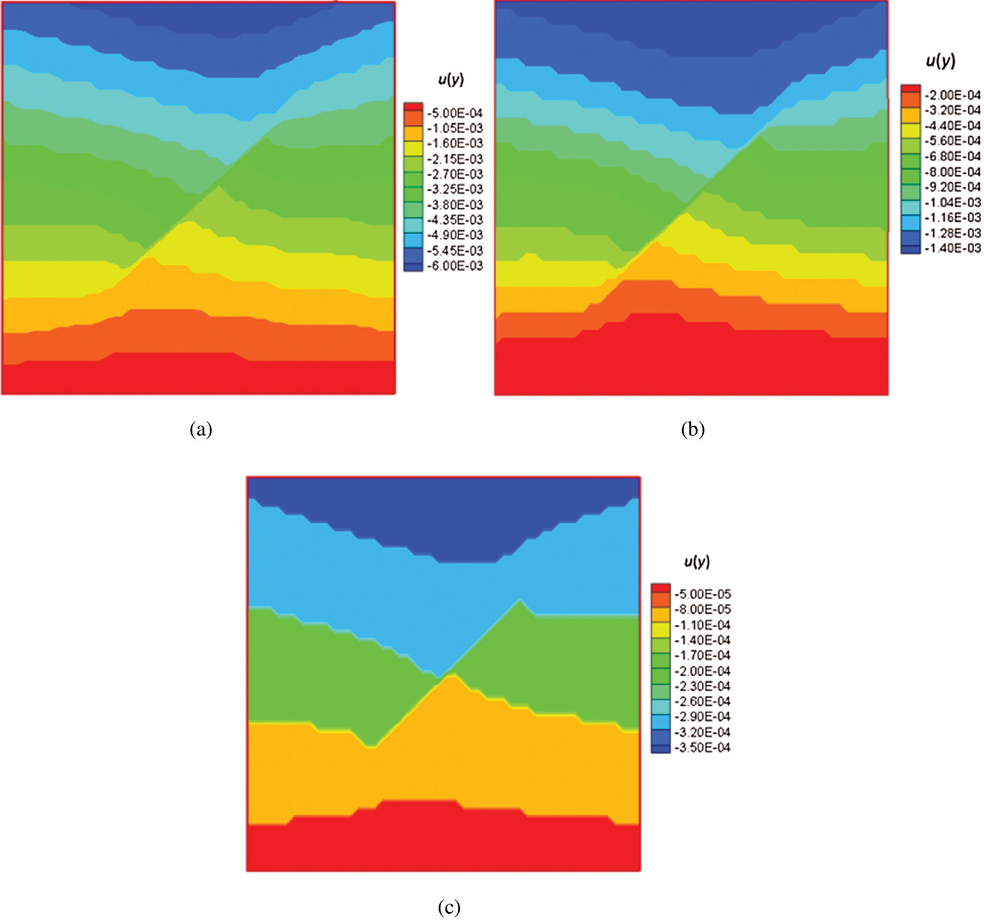
: Contours of vertical displacement of the reservoir with three different Young’s moduli(color bar in units of meters). (a) E = 5 GPa. (b) E = 20 GPa. (c) E = 80 GPa

The distribution of stresses around the fracture can be seen in Figs. 8 and 9; negative values are compressional, positive values are tensile. The minimum principal stress contains both compressive and tensile components, showing that locally the minimum principal stresses change from compressive to tensile near the crack tip, whereas all maximum principal stresses remain compressive.

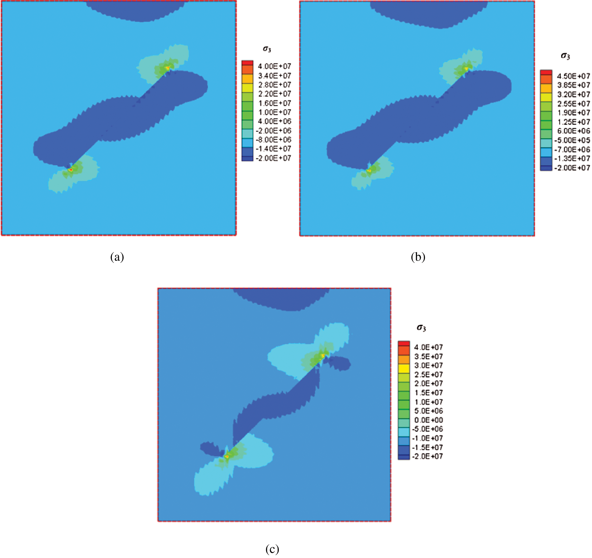
Figure 8: Contours of minimum principal stress for different Young’s moduli (color bar in units of Pa). (a) E = 5 GPa. (b) E = 20 GPa. (c) E = 80 GPa

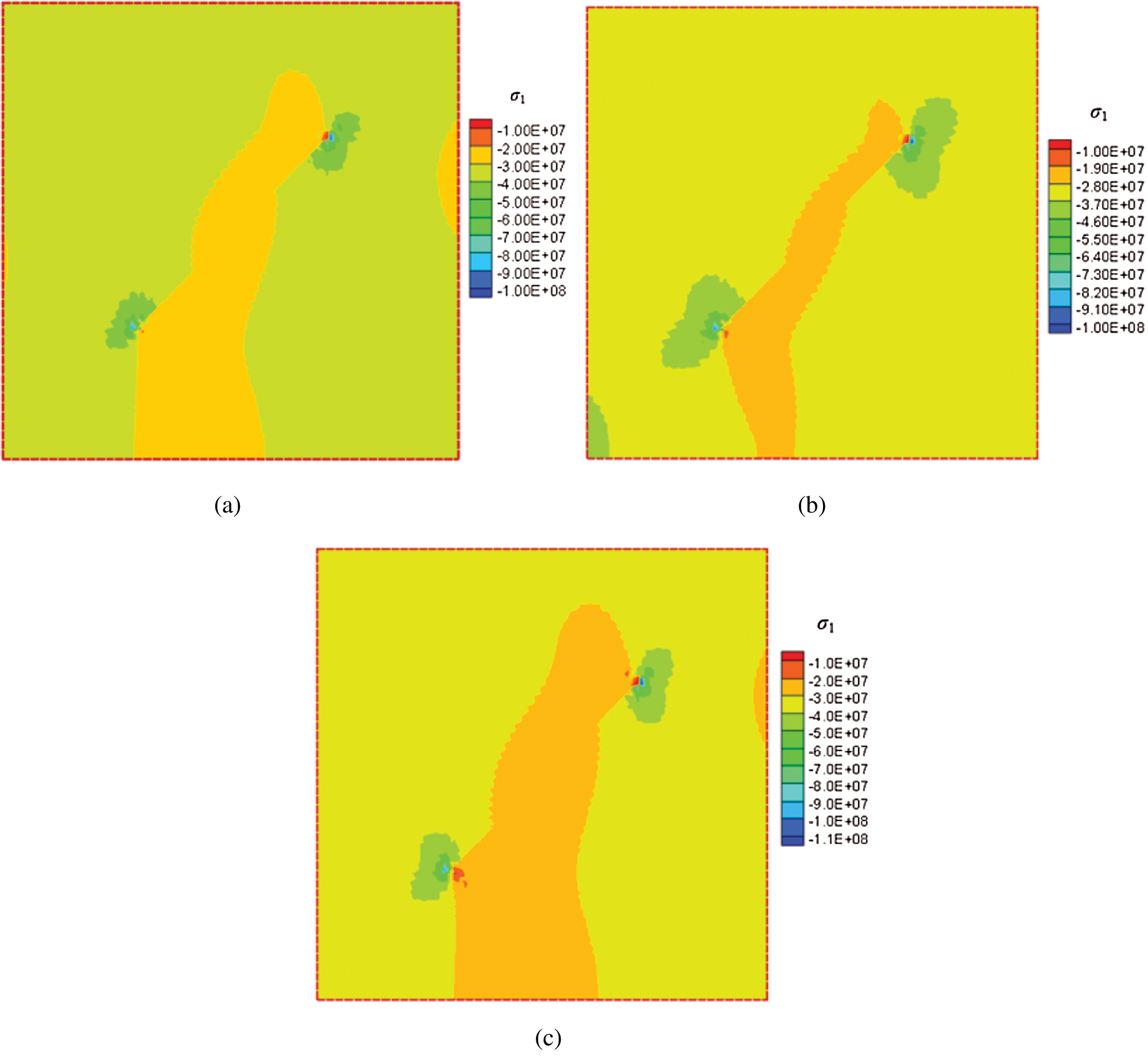
Figure 9: Contours of maximum principal stress for different Young’s moduli (color bar in units of Pa). (a) E = 5 GPa. (b) E = 20 GPa. (c) E = 80 GPa

4.2 The Effect of the Orientation of the Fracture

The displacement field is plotted in Figs. 10 and 11 for different fracture angles, and the slip displacement curve along the fracture for the reservoir with different angles is given in Fig. 12. When the fracture is parallel to the horizontal direction, the fracture remains closed and without slip, as the deviatoric stress (shear stress) on the fracture surface is zero. When the angle between the fracture and the horizontal direction increases to , relative movement along the fracture is noted, as slip takes place, also reorienting the local principal stress directions. When the angle increases to , relative movement along the fracture still takes place, and the slip displacement is larger compared to that of the angle of . However, when the angle turns to from , the slip displacement becomes smaller, indicating that slip is suppressed. As the angle approaches (Figs. 10d and 10e, Figs. 11d and 11e), slip is again suppressed. In other words, there is a range of angles of inclination of the fracture to the principal stress where slip is possible, and this is dictated by the in situ principal stress field and the values of the parameters in the Mohr–Coulomb slip criterion.

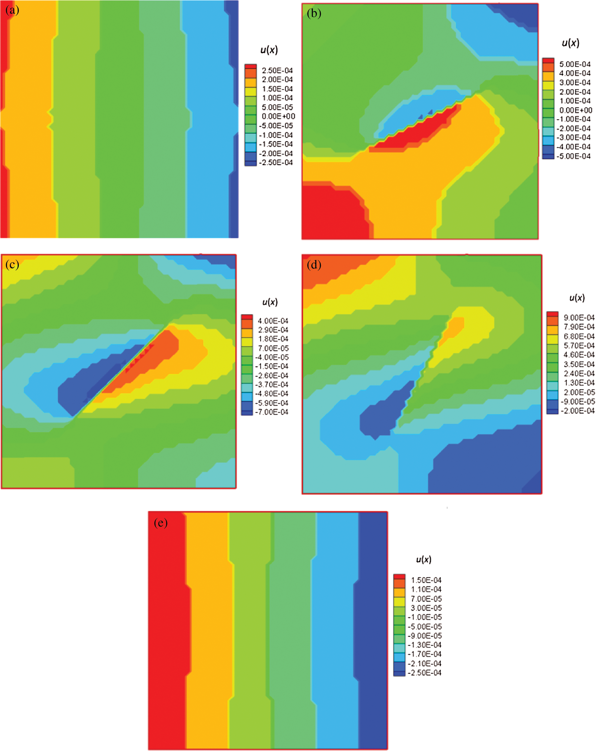
Figure 10: Contours of horizontal displacement for the reservoir with different angles (color bar in units of meters). (a) . (b) . (c) . (d) . (e)

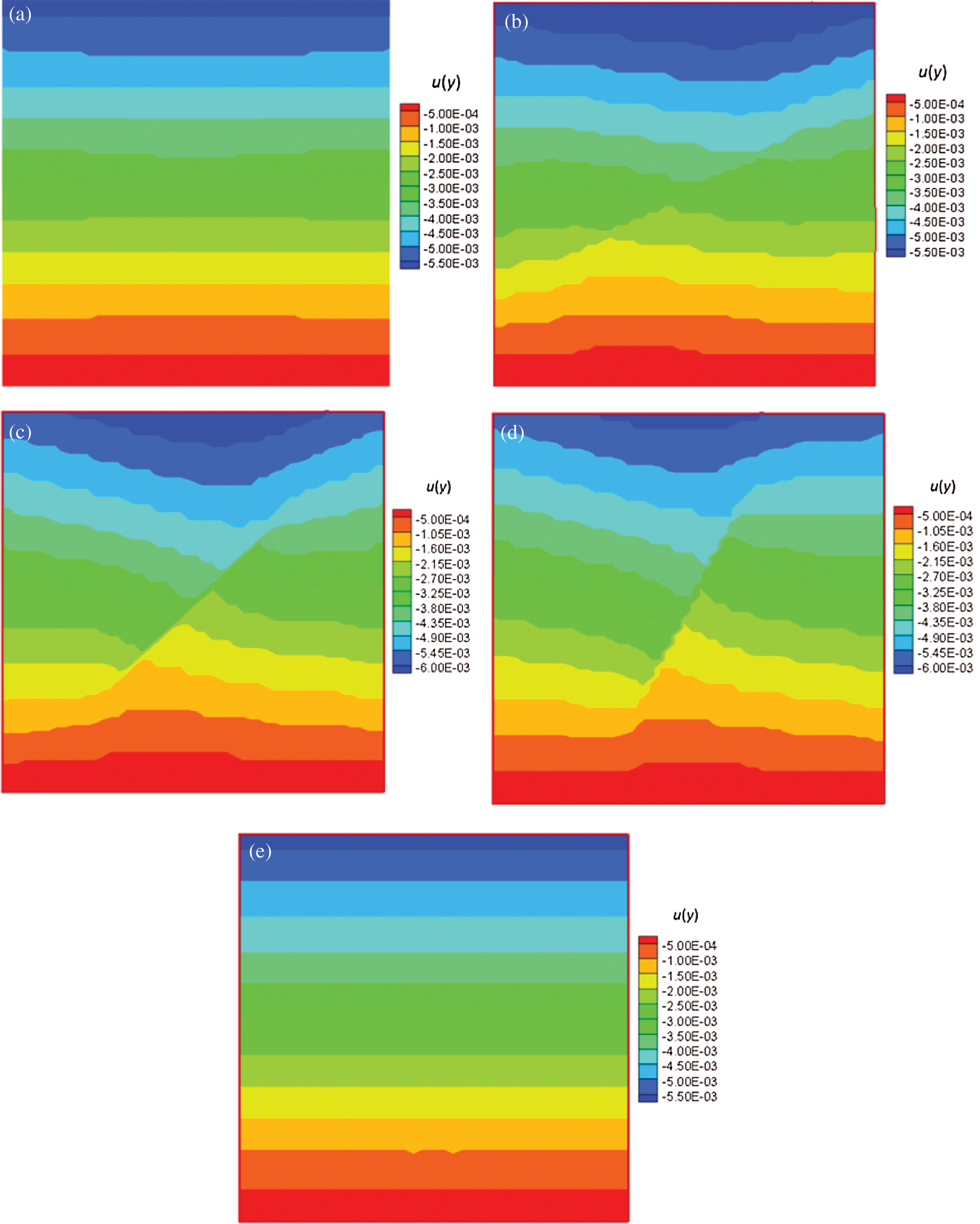
Figure 11: Contours of vertical displacement for the reservoir with different angles (color bar in units of meters). (a) . (b) . (c) . (d) . (e)

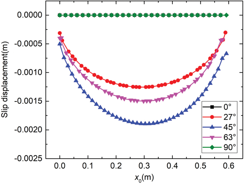
Figure 12: The slip displacement curve along the fracture for the reservoir with different angles (x0-the distance from the left tip point along the fracture; slip displacement-the relative displacement around the two surfaces along the fracture)

Fig. 13 shows the effect of the angle of the fracture in a principal stress field with the fracture Mohr–Coulomb (MC) slip criterion. As stresses change (in this case through some unspecified process), an oriented fracture may slip only within a band of orientations, shown in the small inset diagram, but specified on the larger MC plot.

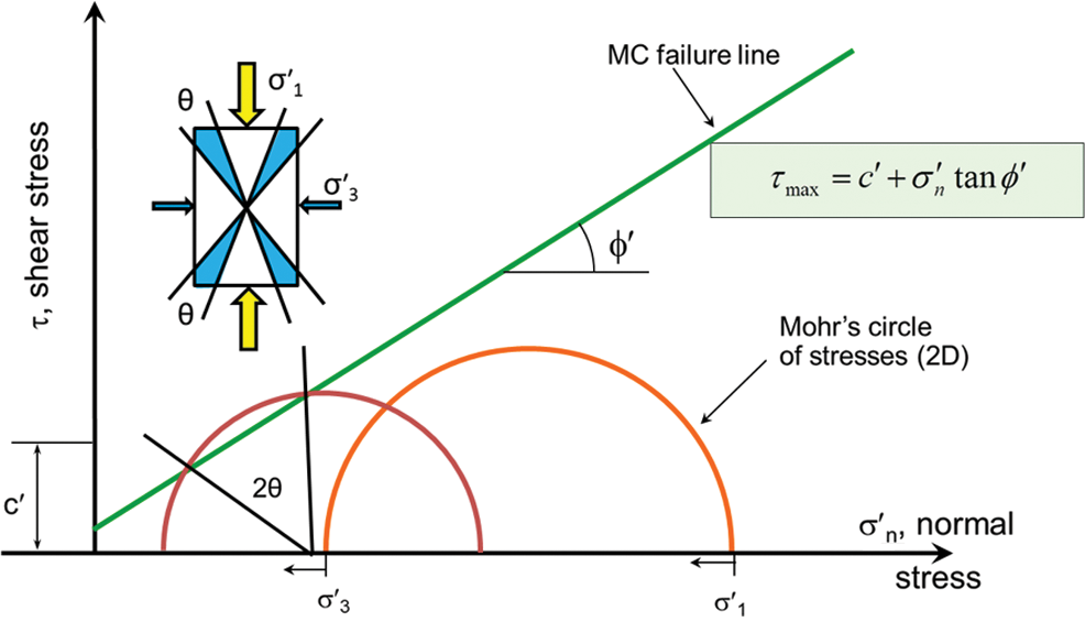
Figure 13: The angle for a slip of a fracture in a principal stress field (, -effective maximum and minimum principal stresses, respectively; -effective normal stress; c′-effective cohesion; ’-effective friction angle; -the angle between the two shear failure surfaces)

4.3 The Effect of the Frictional Coefficient of the Fracture

The horizontal and vertical displacements for different cases where the fracture has different frictional coefficients are shown in Figs. 14 and 15. When the frictional coefficient is as small as 0.1 (a very low friction angle in the Mohr–Coulomb diagram), the discontinuity is large and will occur over a larger range of fracture angles. In this example, the discontinuity slip is suppressed as the frictional coefficient increases to 0.3 and higher, and disappears when the frictional coefficient reaches 0.6. Corresponding stress contours are shown in Figs. 16 and 17.

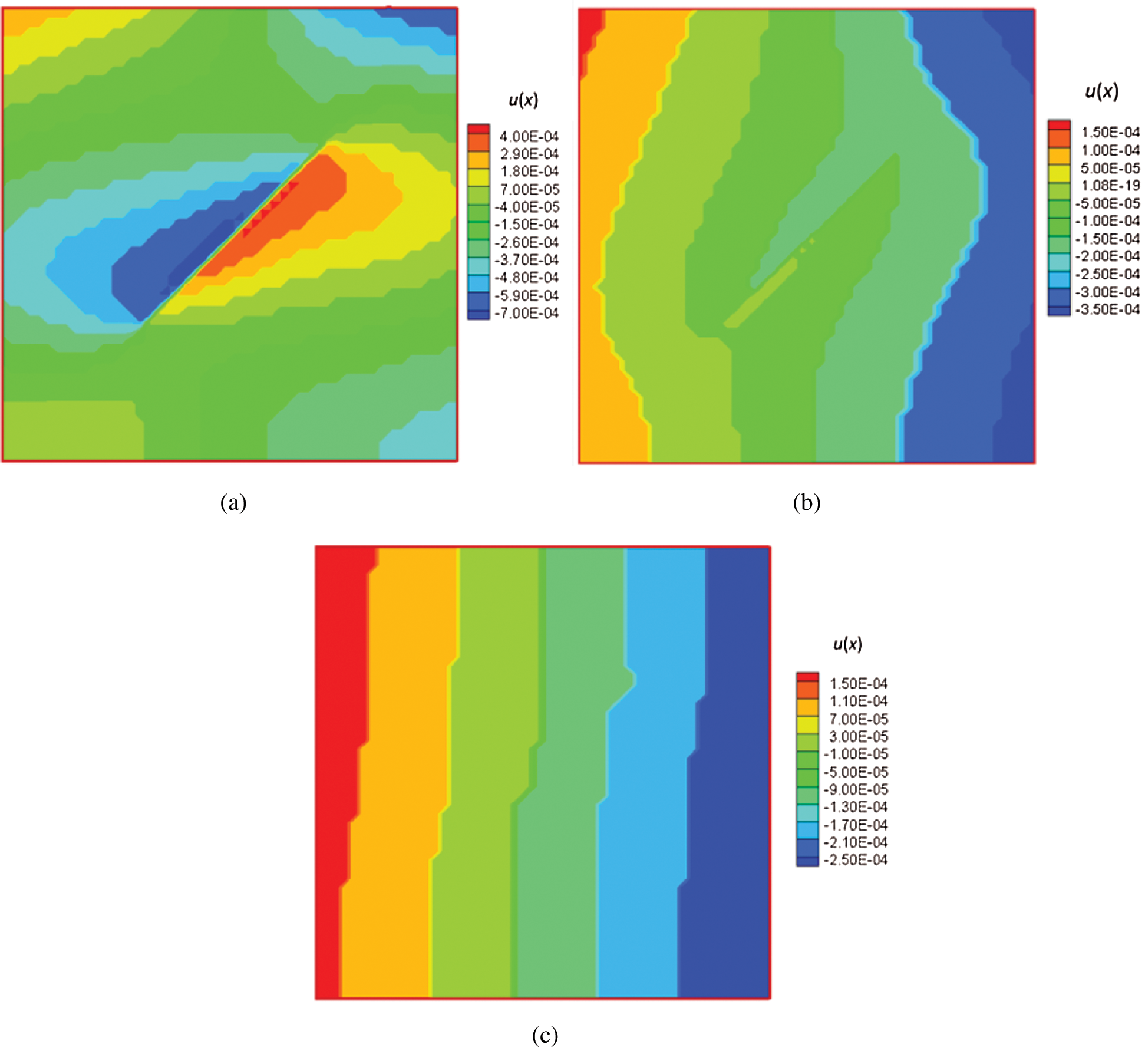
Figure 14: Contours of horizontal displacements for the reservoir with different frictional coefficients (color bar in units of meters). (a) f = 0.1 (b) f = 0.3 (c) f = 0.6

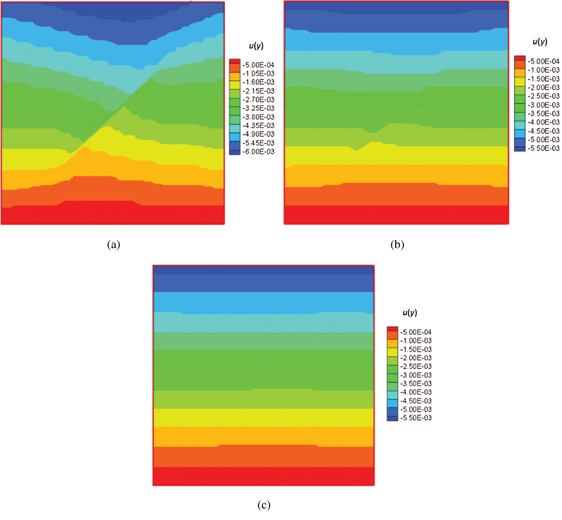
Figure 15: Contours of vertical displacement for the reservoir with different frictional coefficients (color bar in units of meters). (a) f = 0.1. (b) f = 0.3. (c) f = 0.6

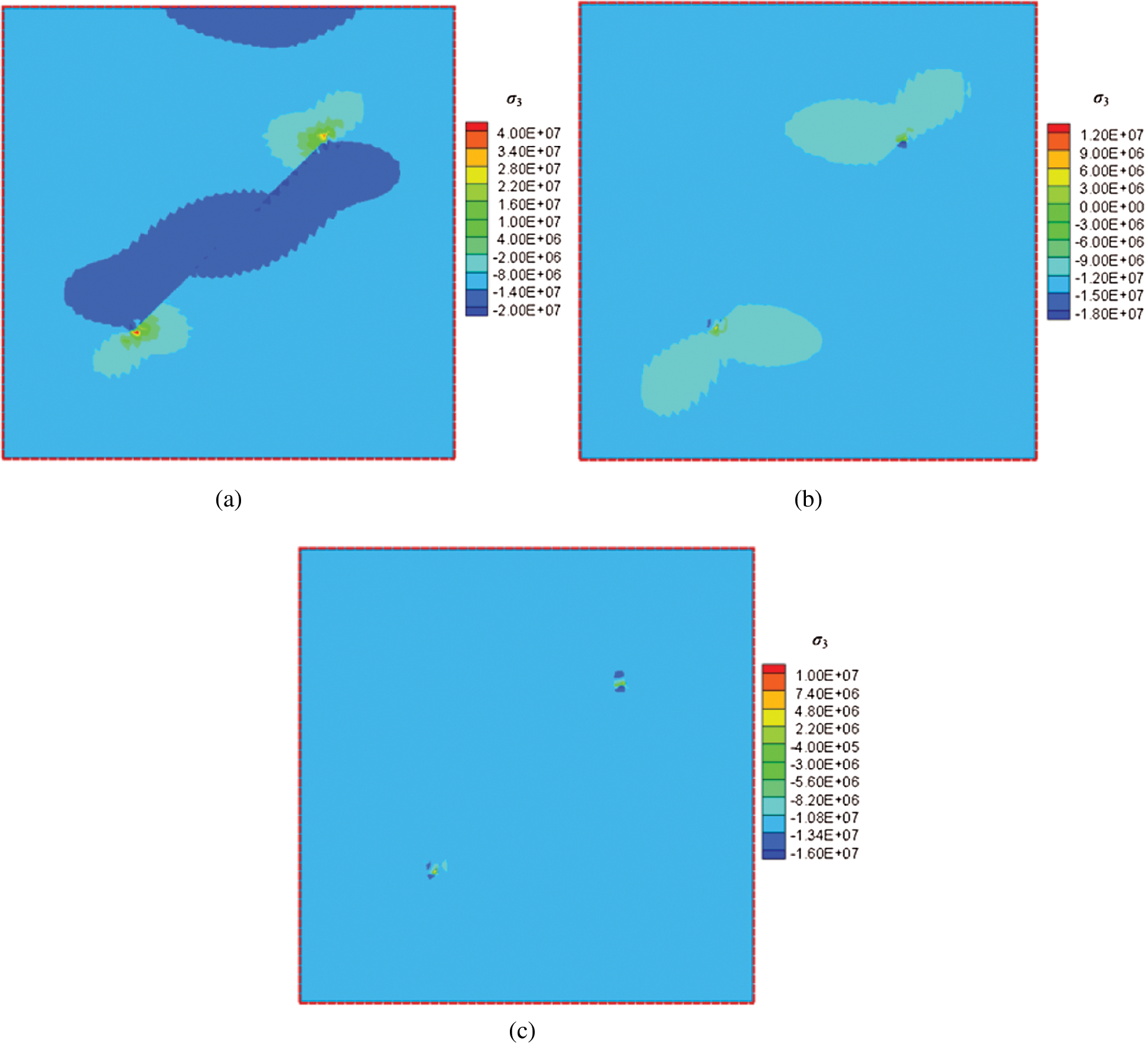
Figure 16: Contours of minimum principal stresses for the reservoir with different frictional coefficients (color bar in units of Pa). (a) f = 0.1 (b) f = 0.3 (c) f = 0.6

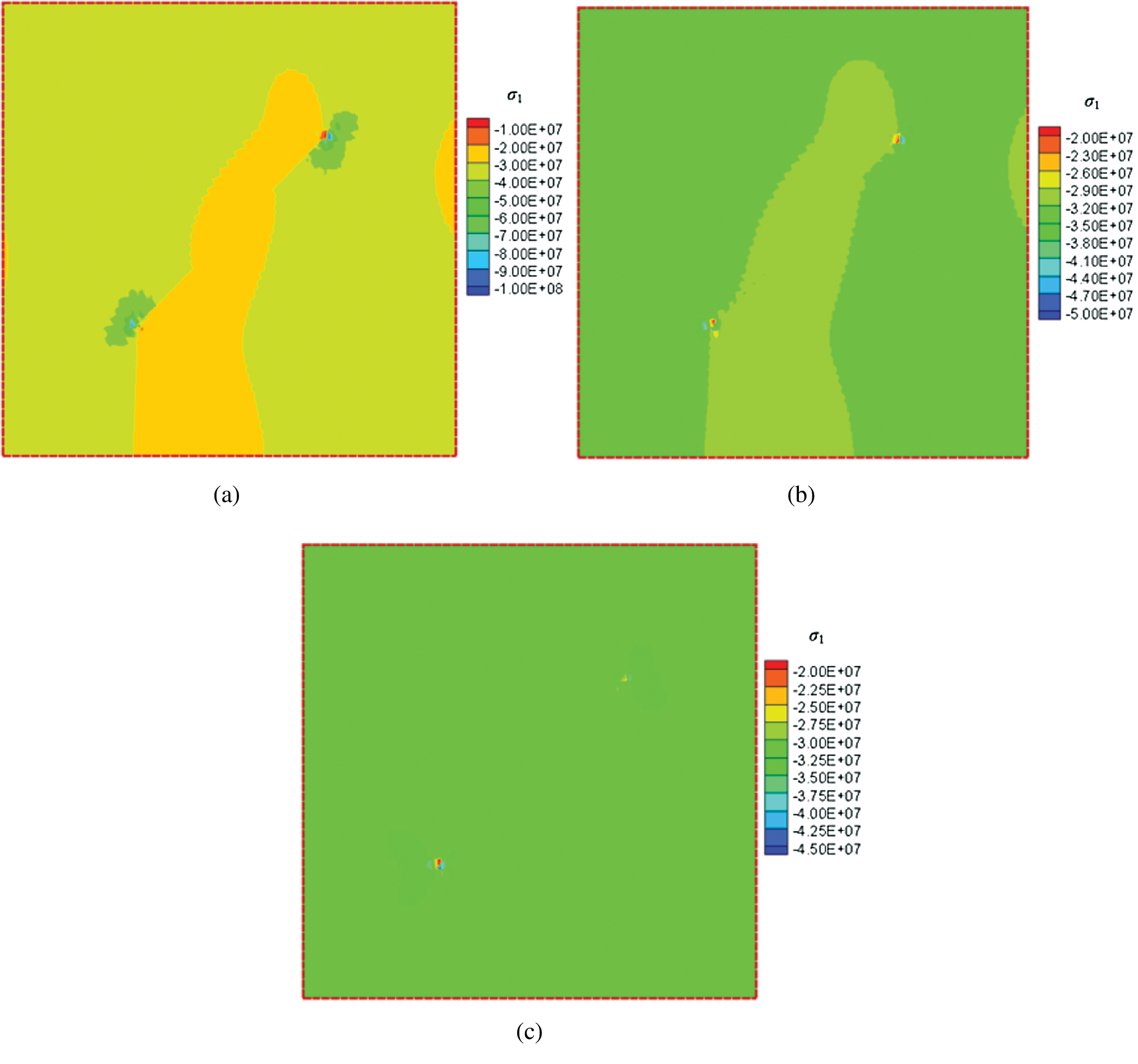
Figure 17: Contours of maximum principal stresses for the reservoir with different frictional coefficients (color bar in units of Pa). (a) f = 0.1 (b) f = 0.3 (c) f = 0.6

5  Conclusions

Using the penalty method, this paper introduces a frictional contact algorithm to XFEM, and a Coulomb friction criterion is employed to govern tangential contact slip. In the numerical experiments, the effect of Young’s modulus, crack orientation, and Coulomb frictional coefficient of the crack surface on the distribution of stress and displacement after depletion of a reservoir are analyzed. The results indicate that depletion-induced shear failure is much more likely to occur in a reservoir of lower Young’s modulus. Also, the angle of the crack (fault, bedding plane, joint) significantly affects the state of stress and displacement, particularly in the vicinity of the crack. Slip only can occur in permitted directions, as determined by the magnitudes of the principal stresses and the frictional coefficient. Finally, a larger frictional coefficient makes the crack less prone to shear failure, and this parameter can be related to the roughness of the slip surface.

Acknowledgement: This research received no external funding.

Author Contributions: Conceptualization, S. D. Yin; methodology, S. D. Yin, M. T. Cao; software, M. T. Cao and S. D. Yin; validation, S. D. Yin and M. T. Cao; writing–original draft preparation, M. T. Cao; writing–review and editing, S. D. Yin, M. B. Dusseault, and W. G. Liang. All authors have read and agreed to the published version of the manuscript.

Funding Statement: The author(s) received no specific funding for this study.

Conflicts of Interest: The authors declare that they have no conflicts of interest to report regarding the present study.

This work is licensed under a Creative Commons Attribution 4.0 International License, which permits unrestricted use, distribution, and reproduction in any medium, provided the original work is properly cited.