| Computer Modeling in Engineering & Sciences |
DOI: 10.32604/cmes.2021.012383
ARTICLE
Lemniscate of Leaf Function
Department of Mechanical Systems Engineering, Daido University, 10-3 Takiharu-cho, Minami-ku, Nagoya, 457-8530, Japan
*Corresponding Author: Kazunori Shinohara. Email: shinohara@06.alumni.u-tokyo.ac.jp
Received: 28 June 2020; Accepted: 14 September 2020
Abstract: A lemniscate is a curve defined by two foci, F1 and F2. If the distance between the focal points of F1 − F2 is 2a (a: constant), then any point P on the lemniscate curve satisfy the equation PF1.PF2 = a2. Jacob Bernoulli first described the lemniscate in 1694. The Fagnano discovered the double angle formula of the lemniscate (1718). The Euler extended the Fagnano’s formula to a more general addition theorem (1751). The lemniscate function was subsequently proposed by Gauss around the year 1800. These insights were summarized by Jacobi as the theory of elliptic functions. A leaf function is an extended lemniscate function. Some formulas of leaf functions have been presented in previous papers; these included the addition theorem of this function and its application to nonlinear equations. In this paper, the geometrical properties of leaf functions at n = 2 and the geometric relation between the angle  and lemniscate arc length l are presented using the lemniscate curve. The relationship between the leaf functions sleaf2 (l) and cleaf2 (l) is derived using the geometrical properties of the lemniscate, similarity of triangles, and the Pythagorean theorem. In the literature, the relation equation for sleaf2 (l) and cleaf2 (l) (or the lemniscate functions, sl (l) and cl (l)) has been derived analytically; however, it is not derived geometrically.
Keywords: Geometry; lemniscate of Bernoulli; leaf functions; lemniscate functions; Pythagorean theorem; triangle similarity
An ordinary differential equation (ODE) comprises a function raised to the 2n −1 power and the second derivative of this function. Further, the initial conditions of the ODE are defined.


Another ODE and its initial conditions are given below:


The ODE comprises a function r(l)(or  ) of one independent variable l(or
  ) and the derivatives of this function. The variable n represents a natural number (
 ). The above equation and the initial conditions constitute a very simple ODE. However, when this differential equation is numerically analyzed, mysterious waves are generated for all natural numbers. These mysterious waves are regular waves with some periodicity and amplitude. If these waves can be explained, they have the potential to solve various problems of nonlinear ODEs.
No elementary functions satisfy Eqs. (1)–(3). Therefore, in this paper, the function that satisfies Eqs. (1)–(3) is defined as cleafn(l). Function r(l) is abbreviated as r. By multiplying the derivative dr/dl with respect to Eq. (1), the following equation is obtained.

The following equation is obtained by integrating both sides of Eq. (7).

Using the initial conditions in Eqs. (2) and (3), the constant  is determined. The following equation is obtained by solving the derivative dr/dl in Eq. (8).

We can create a graph with the horizontal axis as the variable l and the vertical axis as the function r. Because function r is a wave with a period, the gradient dr/dl has positive and negative values, and it depends on domain l. In the domain,  (See Appendix A for the constant
  ), the above gradient dr/dl becomes negative.

The following equation is obtained by integrating the above equation from 1 to r.

For integrating the left side of the above equation, the initial condition (Eq. (2), (l, r) = (0, 1)) is applied. The above equation represents the inverse function of the leaf function: cleafn(t) [1]. Therefore, the above equation is described as

Similarly, the function that satisfies Eqs. (4)–(6) is defined as sleaf . In the domain,
  (See Appendix A for constant
  ), the gradient
  becomes positive.

The following equation is obtained by integrating the above equation from 0 to  .
.

For integrating the left side of the above equation, the initial condition (Eq. (5), (l, r) = (0, 0)) is applied. The above equation represents the inverse function of the leaf function: sleaf [2]. Therefore, the above equation is described as

Inverse leaf functions based on the basis n = 1 represent inverse trigonometric functions.


In 1796, Carl Friedrich Gauss presented the lemniscate function [3]. The inverse leaf functions based on the basis n = 2 represents inverse functions of the sin and cos lemniscates [4].


In 1827, Jacobi [5] presented the Jacobi elliptic functions. Compared to Eq. (18), the term t2 is added to the root of the integrand denominator.

Eq. (20) represents the inverse Jacobi elliptic function sn, where k is a constant; there are 12 Jacobi elliptic functions, including cn and dn, etc. In Eq. (20), variable t is raised to the fourth power in the denominator. Jacobi did not discuss variable t raised to higher powers as indicated below.

Thus, historically, the inverse functions have not been discussed in the case of  or higher [6–14].
A lemniscate is a curve defined by two foci F1 and F2. If the distance between the focal points of F1 − F2 is 2a (a: constant), then any point P on the lemniscate curve satisfies the equation  . Jacob Bernoulli first described the lemniscate in 1694 [15,16]. Based on the lemniscate curve, its arc length can be bisected and trisected using a classical ruler and compass [17]. Based on this lemniscate, a lemniscate function was proposed by Gauss around the year 1800 [3,18]. Nishimura proposed a relationship between the product formula for the lemniscate function and Carson’s algorithm; it is known as the variant of the arithmetic–geometric mean of Gauss [19,20]. The Wilker and Huygens-type inequalities have been obtained for Gauss lemniscate functions [21]. Deng et al. [22] established some Shafer–Fink type inequalities for the Gauss lemniscate function. The geometrical characteristics of the lemniscate have been described [23,24]. Mendiratta et al. [25] investigated the geometric properties of functions. Levin [26] developed analogs of sine and cosine for the curve to prove the formula. Langer et al. [27] presented the lemniscate octahedral groups of projective symmetries. As a kinematic control problem, a five body choreography on an algebraic lemniscate was shown as the potential problem for two values of elliptic moduli [28]. The trajectory generation algorithm was applied by using the shape of the Bernoulli lemmiscate [29].
Leaf functions are extended lemniscate functions. Various formulas for leaf functions such as the addition theorem of the leaf functions and its application to nonlinear equations have been presented [30–32].
In this paper, the geometrical properties of leaf functions for n = 2, and the geometric relationship between the angle  and lemniscate arc length l are presented using the lemniscate curve. The relations between leaf functions
  and
and  are derived using the geometrical properties of the lemniscate curve, similarity of triangles, and the Pythagorean theorem. In the literature, the relationship equation of
  and
and  is analytically derived; however, it is yet to be derived geometrically [33]. The relation between
  and
and  can be expressed as

The Eq. (22) was analytically derived. However, it cannot be geometrically derived using the lemniscate curve because it is not possible to show the geometric relationship of the lemniscate functions sl (l) and cl (l) on a single lemniscate curve. In contrast, phase l of the lemniscate function and angle  can be visualized geometrically on a single lemniscate curve. Therefore, in the literature, Eq. (22) is derived using an analytical method without requiring the geometric relationship.
In this paper, the angle  , phase l, and leaf functions
  and
and  (or lemniscate functions sl(l) and cl(l)) are visualized geometrically on a single lemniscate curve. Eq. (22) is derived based on the geometrical interpretation, similarity of triangles, and Pythagorean theorem.
2 Geometric Relationship with the Leaf Function 
Fig. 1 shows the geometric relationship between the lemniscate curve and  . The y and x axes represent the vertical and horizontal axes, respectively. The equation of the curve is

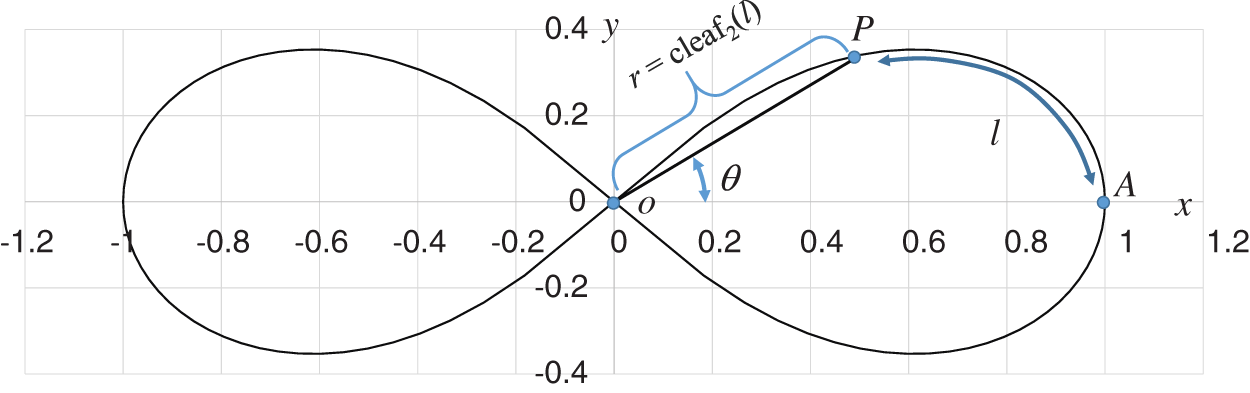
Figure 1: Geometric relationship between angle  and phase l of the leaf function
If P is an arbitrary point on the lemniscate curve, then the following geometric relation exists.


When point P is circled along the contour of one leaf, the contour length corresponds to the half cycle  (See Appendix A for the definition of the constant
  ). As shown in Fig. 1, with respect to an arbitrary phase l, angle
  must satisfy the following inequality.

Here, k is an integer.
3 Geometric Relationship between the Trigonometric Function and Leaf Function 
Fig. 2 shows the foci F and F of the lemniscate curve. The length of a straight line connecting an arbitrary point
  and one focal point
  is denoted by
  . Similarly,
  denotes the length of the line connecting an arbitrary point
  and a second focal point
  . On the curve, the product of
  and
and  is constant. The relationship equation is described as [34]

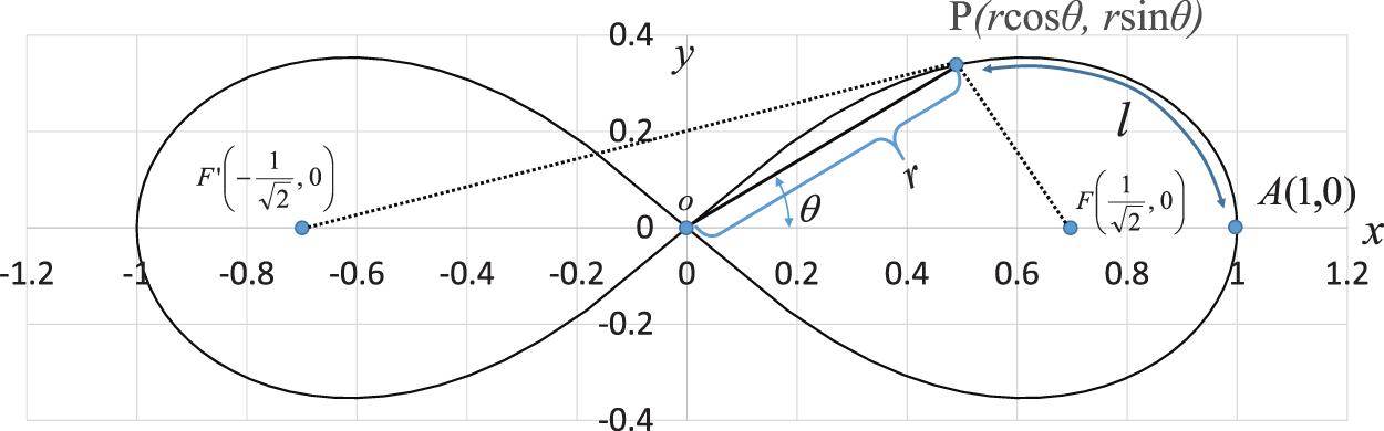
Figure 2: Lemniscate focus
The coordinates of point P are

 and
and  are given by
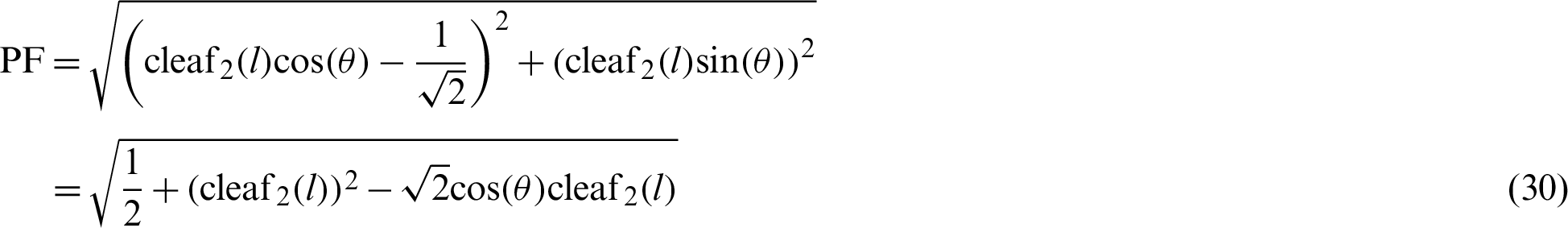
and
respectively.
By substituting Eqs. (30) and (31) into Eq. (28), the relationship equation between the leaf function  and trigonometric function
  can be derived as

After differentiating Eq. (32) with respect to l,

The following equation is obtained by combining Eqs. (32) and (33).
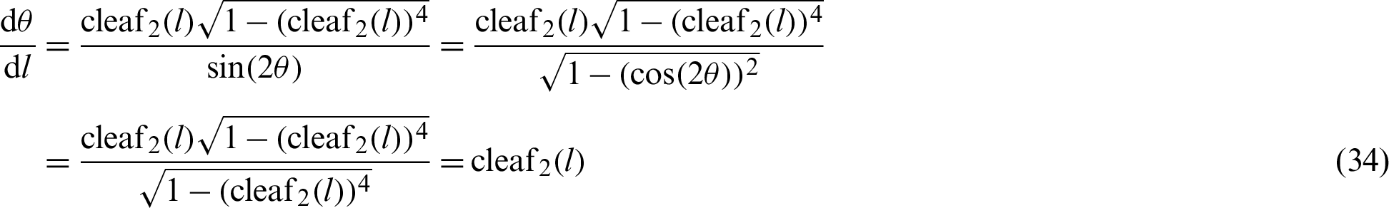
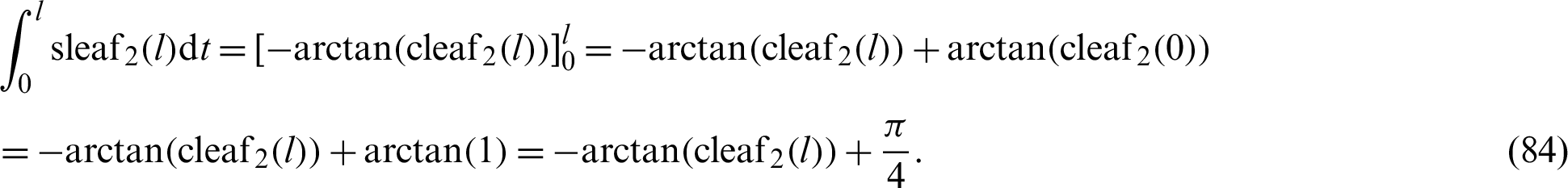
The differential equation can be integrated using variable l. Parameter t in the integrand is introduced to distinguish it from l. The integration of Eq. (34) in the region  yields the following equation (See Appendix C for details).

Therefore, the following equation holds.

Eq. (32) can only be described by variable l as

The phase  of the cos function is plotted in Fig. 3 through numerical analysis. The horizontal and vertical axes represent variables l and
  , respectively. As shown in Fig. 3, angle
  satisfies the inequality

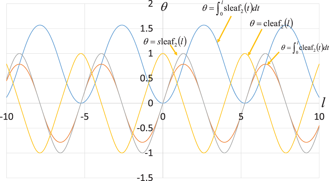
Figure 3: Curves of leaf functions ( and
and  ) and the integrated leaf functions (
 and
and  )
)
Eq. (38) satisfies the inequality of Eq. (27) under the condition k = 0.
Fig. 4 shows the geometric relationship between functions  and
and  . The geometric relation in Eq. (36) is illustrated in Fig. 4.
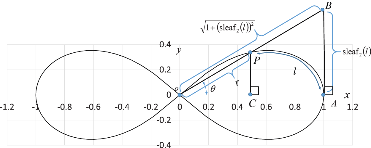
Figure 4: Geometric relationship between leaf functions  and
and 
Draw a perpendicular line from the point P on the lemniscate to the x-axis. This perpendicular is parallel to the y-axis. Let C be the intersection of this perpendicular and the x-axis. Therefore, the angle  OCP is 90
 . Next, draw a line perpendicular to the x-axis from the intersection A(1,0) of the lemniscate and the x-axis. Let B be the intersection of this perpendicular and the extension of the straight line OP. Here,
  and
and  . Substituting these into Eq. (23) gives


and

P and B are moving points, and point A is fixed. When angle  is zero, both P and B are at A. The geometric relationship is then expressed as
  OA and sleaf2(l) = 0 = AB. As
  increases, P moves away from A, and it moves along the lemniscate curve. Here, phase l of cleaf2(l) and sleaf2(l) corresponds to the length of the arc
  . The length of the straight line OP is equal to the value of cleaf2(l). Point B is the intersection point of the straight lines OP and x = 1. In other words, P is the intersection point of the straight line OB and lemniscate curve. As
  increases, B moves away from A and onto the straight line x = 1. That is, it moves in the direction perpendicular to the x axis. The length of straight line AB is equal to the value of sleaf2(l). When
  reaches
  , P moves to origin O and
  . The length of arc
  (or phase l) is
  . Moreover, cleaf2(l) = 0 = OP and sleaf2(l) = 1 = AB.
The relationship  is derived by the similarity of triangles
  , as shown in Fig. 4. Thus, the following equation holds.
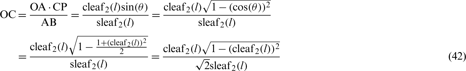
Eq. (32) is applied in the transformation process. Similarly, the relationship  is derived by the similarity of triangles
  , as shown in Fig. 4. Therefore, the following equation holds.

By substituting Eqs. (42) and (43) into Eq. (39), the following equation is obtained.
By rearranging Eq. (44), the following equation is obtained.


For arbitrary l,  and
and  . The relationship between
  and
and  can then be obtained as Eq. (22).
4 Geometric Relationship of the Leaf Function 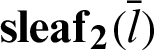
Fig. 5 shows the geometric relationship between length  and lemniscate curve inclined at
  . In Fig. 5, the y and x axes represent the vertical and horizontal axes, respectively. The equation of this curve is given as

Figure 5: Geometric relationship between angle  and phase
  of leaf function
If  is an arbitrary point on the lemniscate curve, the following geometric relation exists.


(See Appendix D)

In Fig. 5, for an arbitrary variable  , the range of angle
  is given by

Here, k is an integer.
5 Geometric Relationship between Trigonometric Function and Leaf Function 
Fig. 6 shows foci  and
and  of the lemniscate curve inclined at an angle of
  . This curve has the same relation equation as shown in Fig. 2.

Figure 6: Lemniscate curve inclined at 
The coordinates of point  on the lemniscate curve inclined at an angle of
  are given as

Lengths  and
and  are expressed by
and
By substituting Eqs. (54) and (55) into Eq. (52), the relationship equation between the leaf function  and the trigonometric function
  can be derived as

The following equation is obtained by differentiating Eq. (56) with respect to the variable  .
.

After applying Eq. (56), the equation is transformed as
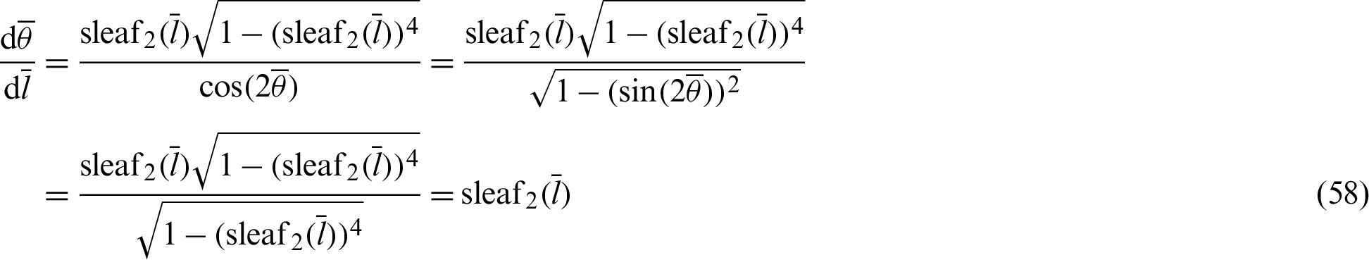
The differential equation is integrated by variable  . Parameter t is introduced to distinguish the parameter from variable
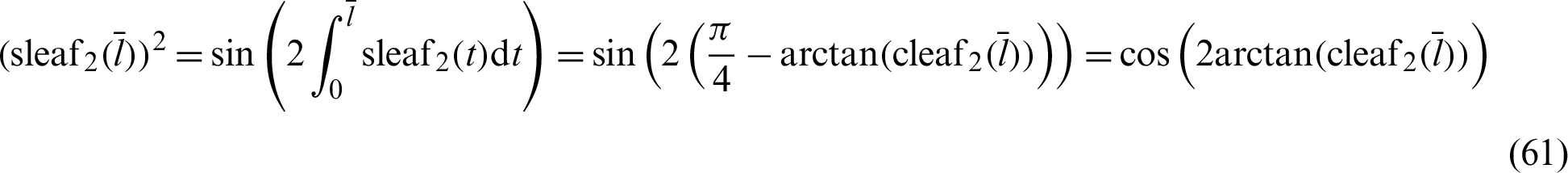
  in the integration region. The integration of Eq. (58) in region
  (See Appendix C) yields

and the following equation holds.

Using Eq. (59), Eq. (56) can be described by variable  as
as
The curve of phase  is plotted in Fig. 3 through numerical analysis. The horizontal and vertical axes represent variables
  and
and  , respectively. As shown in Fig. 3, angle
  satisfies the following range.

Eq. (62) satisfies the range of Eq. (51) under the condition k = 0. Fig. 7 shows the lemniscate curve inclined at  . The geometric relation of Eq. (60) is added to Fig. 7.


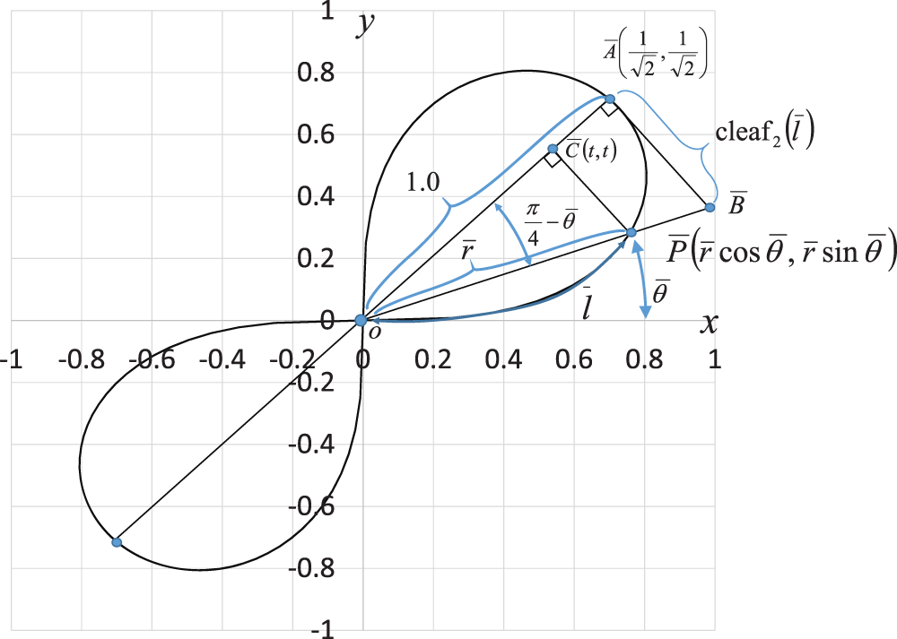
Figure 7: Geometric relationship based on the lemniscate curve inclined at 
Let 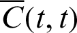 be the coordinates on line
  , as shown in Fig. 7. Points
  and
and  are moving points, and point
  is fixed. When angle
  is zero,
  is at origin O, and
  is on the x-axis at
  . The geometric relationship is described as
  and sleaf
 . As
. As  increases,
  moves away from origin O and along the lemniscate curve. The phase
  of both cleaf
 and sleaf
 corresponds to the length of arc
  . The length of the straight line
  is equal to the value of sleaf
 . Point
  is the intersection point of straight lines
  and
and  . In other words,
  is the intersection point of the straight line
  and the lemniscate curve. As
  increases,
  moves away from point
  ,0) on a straight line
  . Here, the length of the straight line
  is equal to the value of cleaf
 . When
  reaches
  ,
,  moves to point
  . The length of arc
  (or phase
  ) becomes
  . Furthermore, cleaf
 and sleaf
 . The linear equation
  is given by

By substituting Eq. (65) into Eq. (47) and solving for variable x, four solutions can be obtained as


As Eqs. (66) and (67) include imaginary numbers, the solutions for x using both Eqs. (68) and (69) are determined by the intersection points of line  and the lemniscate curve, as shown in Fig. 7. The larger x value is given by Eq. (69). That is, the coordinates of point
  can be expressed as

Therefore, the length  is expressed as

The following equation is obtained from the Pythagorean theorem of the triangle  .
.

Substitution of Eqs. (48) and (71) into Eq. (72) yields

The length ratio is 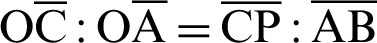 owing to the similarity of triangles
 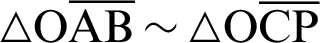 .
.

The elimination of variable t from Eqs. (73) and (74) yields the relation equation, Eq. (22).
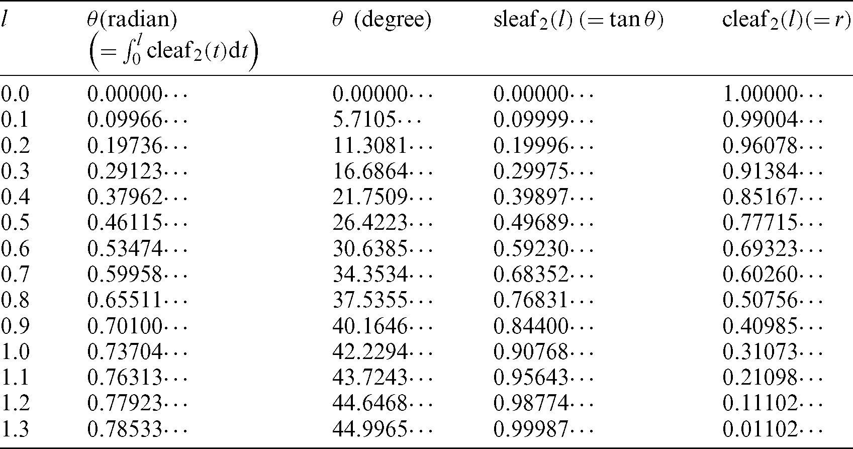
Tab. 1 lists the numerical values for Fig. 4. The angle  and values of the leaf function (sleaf2(l) and cleaf2(l)) are calculated along the arc length l. The values of leaf functions cleaf2(l) are calculated by Eqs. (1)–(3). The values of leaf functions sleaf2(l) are calculated by Eqs. (4)–(6). Based on these data, the numerical data of functions sleaf2(l) and cleaf2(l) can be confirmed using Eq. (22). The function cleaf2(l) (= r) can also be confirmed by using Eq. (82). Angle
  can be calculated by using Eq. (35).
Table 1: Numerical data of arc length l, angle  , and leaf functions sleaf2(l) and cleaf2(l) for Fig. 4
Tab. 2 shows the numerical values for Fig. 7. The angle  and the values of leaf function (sleaf
 and cleaf
 ) are calculated along the arc length
  . Based on these data, the function sleaf
 can also be confirmed using Eq. (90). The angle
  can be calculated using Eq. (59).
Table 2: Numerical data of arc length  , angle
  , and leaf functions sleaf
 and cleaf
 for Fig. 7
Based on the geometric properties of the lemniscate curve, the geometric relationship among angle  , lemniscate length l, and leaf functions
  and
and  were shown on the lemniscate curve. Using the similarity of triangles and the Pythagorean theorem, the relationship equation of leaf functions
  and
and  was derived.
Acknowledgement: The author gratefully acknowledges the helpful comments and suggestions of the reviewers that have improved the presentation of this paper.
Funding Statement: This research is supported by Daido University research Grants (2020).
Conflicts of Interest: The authors declare that they have no conflicts of interest to report regarding the present study.
1. Shinohara, K. (2016). Special function: Leaf function (second report). Bulletin of Daido University, 51, 39–68. [Google Scholar]
2. Shinohara, K. (2016). Special function: Leaf function (first report). Bulletin of Daido University, 51, 23–38. [Google Scholar]
3. Gauss, C. F., Clarke, A. A. (1965). Disquisitiones arithmeticae. United Kingdom: Yale University Press. [Google Scholar]
4. Roy, R. (2017). Elliptic and modular functions from Gauss to Dedekind to Hecke. United Kingdom: Cambridge University Press. [Google Scholar]
5. Jacobi, C. G. J. (2010). Opuscula mathematica. In: Mathematische werke. Berlin: Nabu Press. [Google Scholar]
6. Booth, J. (1852). Researches on the geometrical properties of elliptic integrals. Philosophical Transactions of the Royal Society of London, 142, 311–416. DOI 10.1098/rstl.1852.0019. [Google Scholar] [CrossRef]
7. Byrd, P., Comfort, W., Friedman, M., Friedman, M., Negrepontis, S. (1971). Handbook of elliptic integrals for engineers and scientists. New York: Springer-Verlag.
8. Akhiezer, N., McFaden, H. (1990). Elements of the theory of elliptic functions. In: Translations of mathematical monographs. Providence: American Mathematical Society.
9. Dixon, A. (1894). The elementary properties of the elliptic functions, with examples. New York, United States: Macmillan.
10. Lawden, D. (1989). Elliptic functions and applications. In: Applied mathematical sciences. Berlin, Germany: Springer.
11. McKean, H., Moll, V. (1999). Elliptic curves: Function theory, geometry, arithmetic. Cambridge, United Kingdom: Cambridge University Press.
12. Walker, P. (1996). Elliptic functions: A constructive approach. England: Wiley.
13. Hancock, H. (1958). Lectures on the theory of elliptic functions: Analysis. In: Dover books on advanced mathematics. United States: Dover Publications.
14. Mickens, R. (2019). Generalized trigonometric and hyperbolic functions. United States: CRC Press. [Google Scholar]
15. Bos, H. J. M. (1974). The lemniscate of Bernoulli. In: Cohen, R. S., Stachel, J. J., Wartofsky, M. W. (Eds.For Dirk Struik: Historical and political essays in honor of Dirk J. Struik, pp. 3–14, Dordrecht: Springer Netherlands. [Google Scholar]
16. Ayoub, R. (1984). The lemniscate and fagnano’s contributions to elliptic integrals. Archive for History of Exact Sciences, 29, 131–149. [Google Scholar]
17. Osler, T. (2016). Bisecting and trisecting the arc of the lemniscate. Mathematical Gazette, 100(549), 471–481. DOI 10.1017/mag.2016.112. [Google Scholar] [CrossRef]
18. Rosen, M. (1981). Abel’s theorem on the lemniscate. American Mathematical Monthly, 88(6), 387–395. DOI 10.1080/00029890.1981.11995279. [Google Scholar] [CrossRef]
19. Nishimura, R. (2015). New properties of the lemniscate function and its transformation. Journal of Mathematical Analysis and Applications, 427(1), 460–468. DOI 10.1016/j.jmaa.2015.02.066. [Google Scholar] [CrossRef]
20. Carlson, B. C. (1971). Algorithms involving arithmetic and geometric means. American Mathematical Monthly, 78(5), 496–505. DOI 10.1080/00029890.1971.11992791. [Google Scholar] [CrossRef]
21. Neuman, E. (2013). On lemniscate functions. Integral Transforms and Special Functions, 24(3), 164–171. DOI 10.1080/10652469.2012.684054. [Google Scholar] [CrossRef]
22. Deng, J. E., Chen, C. P. (2014). Sharp shafer-fink type inequalities for Gauss lemniscate functions. Journal of Inequalities and Applications, 2014(1), 496. DOI 10.1186/1029-242X-2014-35. [Google Scholar] [CrossRef]
23. Smadja, I. (2008). La lemniscate de fagnano et la multiplication complexe. HAL-SHS (Sciences de l’Homme et de la Société), https://halshs.archives-ouvertes.fr/. [Google Scholar]
24. Schappacher, N. (1997). Some milestones of lemniscatomy. Algebraic geometry (ankara, 1995Lecture notes in pure and applied mathematics, vol. 193, pp. 257–290, New York: Dekker. [Google Scholar]
25. Mendiratta, R., Nagpal, S., Ravichandran, V. (2014). A subclass of starlike functions associated with left-half of the lemniscate of Bernoulli. International Journal of Mathematics, 25(9), 1450090. DOI 10.1142/S0129167X14500906. [Google Scholar] [CrossRef]
26. Levin, A. (2018). A geometric interpretation of an infinite product for the lemniscate constant. American Mathematical Monthly, 113(6), 510–520. DOI 10.1080/00029890.2006.11920331. [Google Scholar] [CrossRef]
27. Langer, J., Singer, D. (2010). Reflections on the lemniscate of Bernoulli: The forty-eight faces of a mathematical gem. Milan Journal of Mathematics, 78(2), 643–682. DOI 10.1007/s00032-010-0124-5. [Google Scholar] [CrossRef]
28. Lopez Vieyra, J. C. (2019). Five-body choreography on the algebraic lemniscate is a potential motion. Physics Letters A, 383(15), 1711– 1715. DOI 10.1016/j.physleta.2019.03.004. [Google Scholar] [CrossRef]
29. Saraiva, R., De Lellis Costa de Oliveira, M., Bruhns Bastos, M., Trofino, A. (2019). An algebraic solution for tracking Bernoullis lemniscate flight trajectory in airborne wind energy systems. IEEE 58th Conference on Decision and Control, Nice, France, pp. 5888–5893. [Google Scholar]
30. Shinohara, K. (2018). Exact solutions of the cubic duffing equation by leaf functions under free vibration. Computer Modeling in Engineering & Sciences, 115(2), 149–215. [Google Scholar]
31. Shinohara, K. (2019). Damped and divergence exact solutions for the duffing equation using leaf functions and hyperbolic leaf functions. Computer Modeling in Engineering & Sciences, 118(3), 599–647. DOI 10.31614/cmes.2019.04472.
32. Shinohara, K. (2020). Addition formulas of leaf functions and hyperbolic leaf functions. Computer Modeling in Engineering & Sciences, 123(2), 441–473. DOI 10.32604/cmes.2020.08656. [Google Scholar] [CrossRef]
33. Markushevich, A. (2014). The remarkable sine functions. New York: Elsevier Science. [Google Scholar]
34. Akopyan, A. (2014). The lemniscate of Bernoulli, without formulas. The Mathematical Intelligencer, 36(4), 47–50. DOI 10.1007/s00283-014-9445-5. [Google Scholar] [CrossRef]
35. Cox, D. A. (2011). Chapter 15–-The lemniscate-galois theory. New Jersey, United States: John Wiley & Sons, Ltd., pp. 457–508. [Google Scholar]
Appendix A
The symbols  are a constant given by

The numerical data of the symbol  are summarized in the Tab. 3.
Appendix B
The Eq. (23) of Cartesian coordinate system is transformed to the following equation of polar coordinates [1,3].

The variable r and  represents OP and
  AOP in Fig. 1. The arc length in the cartesian and polar coordinates is given by

The arc length l of the lemniscate with polar coordinates is given by

By differentiating Eq. (76) with respect to variable  ,
,

Then, by applying Eq. (79),

The following equation is applied to Eq. (80).

Hence, the arc length l becomes

Appendix C
The following function is differentiated.

Integration of the above mentioned equation with respect to l yields
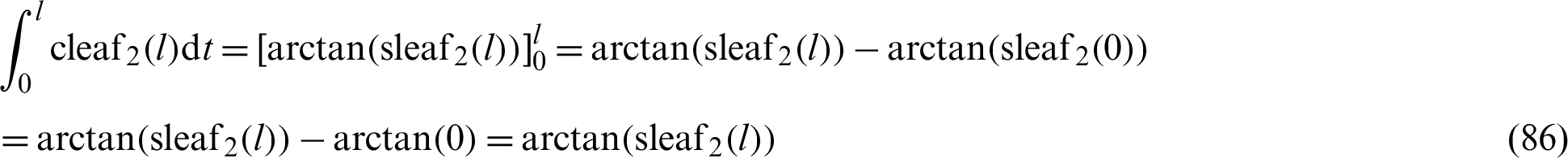
Similarly, the following function is differentiated with respect to variable l.

The following equation is obtained by integrating Eq. (85) with respect to l.
Appendix D
Eq. (47) of the Cartesian coordinate system is transformed to the following equation in the polar coordinates [2,35].

By differentiating Eq. (87) with respect to the variable  ,
,

Then, applying Eq. (88),

Hence, the arc length  becomes

 | This work is licensed under a Creative Commons Attribution 4.0 International License, which permits unrestricted use, distribution, and reproduction in any medium, provided the original work is properly cited. |
