| Computer Modeling in Engineering & Sciences |
DOI: 10.32604/cmes.2021.012821
ARTICLE
Isogeometric Boundary Element Analysis for 2D Transient Heat Conduction Problem with Radial Integration Method
1College of Architecture and Civil Engineering, Xinyang Normal University, Xinyang, 464000, China
2Department of Mechanical Engineering, Suzhou University of Science and Technology, Suzhou, 215009, China
3Key Laboratory of In-Situ Property-Improving Mining of Ministry of Education, Taiyuan University of Technology, Taiyuan, 030024, China
4Institute for Computational Engineering, Faculty of Science, Technology and Communication, University of Luxembourg, Luxembourg
5The York Management School, University of York, York, YO10 5GD, UK
6College of Mechanics and Materials, Hohai University, Nanjing, 211100, China
*Corresponding Author: Haojie Lian. Email: haojie.lian@outlook.com
Received: 16 July 2020; Accepted: 04 September 2020
Abstract: This paper presents an isogeometric boundary element method (IGABEM) for transient heat conduction analysis. The Non-Uniform Rational B-spline (NURBS) basis functions, which are used to construct the geometry of the structures, are employed to discretize the physical unknowns in the boundary integral formulations of the governing equations. Bézier extraction technique is employed to accelerate the evaluation of NURBS basis functions. We adopt a radial integration method to address the additional domain integrals. The numerical examples demonstrate the advantage of IGABEM in dimension reduction and the seamless connection between CAD and numerical analysis.
Keywords: Isogeometric analysis; NURBS; boundary element method; heat conduction; radial integration method
Isogeometric analysis (IGA) has drawn extensive attentions in engineering science community since the seminal works of Hughes et al. [1]. As an alternative to the traditional analysis based on Lagrange polynomial, IGA uses the same spline functions that are used in the geometric expression in CAD, for example Non-Uniform Rational B-splines (NURBS), as the basis functions to approximate the unknown field. Hence, IGA is able to perform numerical analysis directly from CAD without cumbersome preprocessing procedure and geometric errors. Additionally, IGA offers high-order continuity and flexible refinement schemes which are particularly attractive in numerical simulation. Due to the aforementioned salient features, IGA has been successfully applied in many fields [2–6]. To facilitate the implementation of IGA, Bézier extraction [7] technique is proposed that enables one to develop IGA codes in existing finite element codes, without changing the program framework. By using the extraction operator, the complicated iterative process for evaluating B-spline basis functions is eliminated, which improves the efficiency of simulation significantly.
Although the concept of IGA was originally proposed in the context of finite element methods, its application in engineering practice is restricted because FEM relies on volume parameterization which conflicts with the boundary representation in CAD field. Mierzwiczak et al. [8] and Fu et al. [9] applied the isogeometric boundary element method to the heat conduction problem, and proposed the origin intensity factor to eliminate the singularity of the integral. The order reduction of POD model for transient heat transfer was studied by Li et al. [10]. Wang et al. [11] solved the three-dimensional elasto-plastic problem by boundary element method. On the contrary, boundary element method (BEM) [12–19] only needs boundary parameterization and thus is compatible with CAD models naturally. The isogeometric analysis with boundary element method (IGABEM) was first applied to potential problems [20] and elasticity analysis [21,22]. Since then, IGABEM has been applied successfully to a wide range of fields, such as heat conduction [23], linear elasticity [24,25], fracture mechanics [26–28], electromagnetics [29], acoustics [30–35], structural optimization [34,36–40], etc.
In this paper, we are aimed to extend the application of IGABEM to heat conduction problems which are an increasingly important topic in many engineering fields. The radial integration method proposed by Gao [41] is incorporated to solve the additional domain integrals. The problems of constant and variable coefficients, transient and steady state of temperature field are studied. The rest of the paper is arranged as follows: Section 2 gives an overview of the B-spline and NURBS basis. Bézier extraction is detailed in Section 3. In Section 4, the boundary integral equation for heat conduction is introduced and the discrete formula derivation of the boundary integral equation, as well as the time marching method are introduced in detail. Section 5 provides two sets of numerical examples to verify the algorithm, followed by the conclusion in Section 6.
For the sake of completeness, the fundamentals of NURBS are briefed in this section. NURBS are generalized from B-splines, whose basis functions are defined over a knot vector which is a monotonic increasing real number sequence, denoted by  where ui is the i-th knot in the vector U. B-spline basis function is evaluated iteratively as:


where p is the order of the polynomial in B-spline basis functions, and n is the number of the basis functions.
The derivative expression of the basis function can be derived as follows:

The B-spline curve is described by the linear combination of NURBS basis functions and the corresponding control points,

where  is the Cartesian coordinates of control points.
Non-uniform rational B-spline (NURBS) basis functions are obtained by introducing the weight coefficient  to rationalize the B-spline basis,

where

Similar to B-splines, the NURBS curve is expressed by:

Since the NURBS basis function adopts the rational form composed of the B-spline basis function and the weight factor  , it is able to exactly express conic curves, such as ellipses and circles.
The computation of IGABEM can be accelerated using Bézier extraction. The idea is to extract linear operators and map the Bernstein polynomial basis functions of Bézier elements to global B-spline basis functions. The linear transformation is defined by a matrix called an extraction operator. The transpose of the extraction operator maps the control points of the global B-spline to that of Bézier curves. The process of Bézier extraction operation is proposed in this work, also see [7].
To perform Bézier decomposition, all internal knots of a knot vector are repeated until their multiplicity equals p. For example, we insert  after the k-th knot of the original knot vector
  . The new knot
  with k > p. The introduction of new knots will bring about changes in the basis functions and the generation of new control points. The relationship between the original control point P and the new control point Q can be deduced:
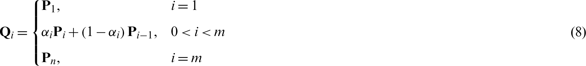
where m = n + 1. The expression for calculating factor  in Eq. (8) is as follows:
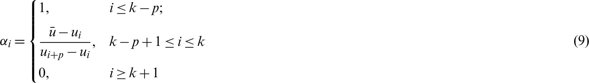
After the knot is inserted, it brings about a change in the control point. Let  be the set of insertion knots required for the Bézier decomposition of the B-spline. Then for each new knot,
  ,
,  , using Eq. (9), we define
  , to be the ith
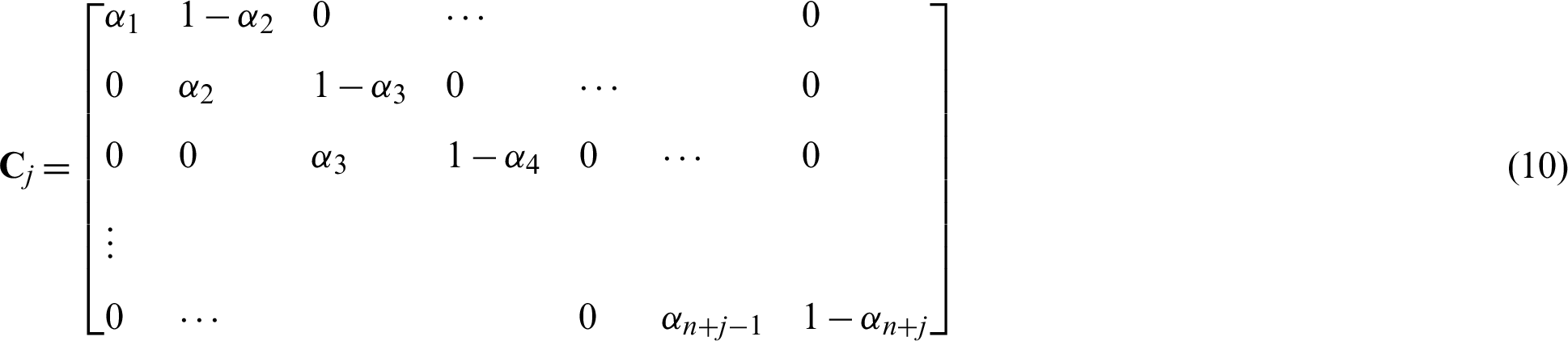
  . So the expression for the conversion matrix C is as follows:
Then, the corresponding control points can be calculated by:

We rewrite Eq. (11) with matrix form:

To decompose a B-spline curve defined in the knot vector  with Bézier extraction, we will insert the knots
  into the existing knot vector. Without changing the geometry, the B-spline curve is expressed using the Bézier basis function as follows:

Using Eqs. (12), (13) can be expressed as follows:

Since  is arbitrary, we can get the following equation

It should be noted that only the knot vector determines the C matrix. In other words, the extraction operator is a product of parameterization and does not depend on control points or basis functions. Therefore, we can apply the extraction operator directly to NURBS. Define weights as diagonal matrices

Converting Eq. (5) to matrix form, we have

Using Eq. (15), the NURBS basis function can be expressed in terms of the Bernstein basis as

The NURBS curve is expressed as:

In Eq. (19),  can be used to express the NURBS curve. Let
  , and define
  to be the diagonal matrix
Eq. (19) can be written as follows:

The expression of the Bézier control points can refer to the method of homogeneous coordinates:

Both sides are multiplied by  at the same time:

After solving the weight factor  and the control point Pb after the Bézier operation, we arrive at the final Bézier representation of the NURBS:

Thus, we can express NURBS equivalently with a series of C0 Bézier elements.
The governing partial differential equation of transient heat conduction in isotropic medium with internal heat source is expressed by:

where T(x, t) represents the temperature at point x at time t, k is the thermal conductivity, b(x, t) shows the heat source value at point x at time t,  is the density of the material, and
  is specific heat capacity.
The following three kinds of boundary conditions are considered:


where  represents the dirichlet boundary,
  the neumann boundary and
  convective boundary condition. n(x) is the unit external normal direction vector at the boundary point.
The transient problem is time-dependent, so the initial conditions need to be prescribed:

where T0 indicates initial temperature on the domain.
4.1 Boundary Element Method of Transient Temperature Field
Through weighted residual operation and partial integration operation, Eq. (25) can be expressed as the following boundary-domain integral equation:

where the coefficient  when the source point x is located in the domain,
  when the source point x is on the boundary of structure, and the integrals are
where  indicates normalized temperature,
  ,
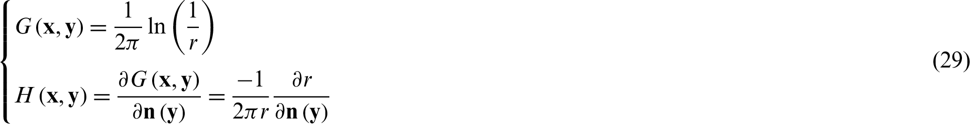
,  is reciprocal of thermal diffusivity, G(x, y) and H(x, y) are Green’s function and it’s derivative, as follows:
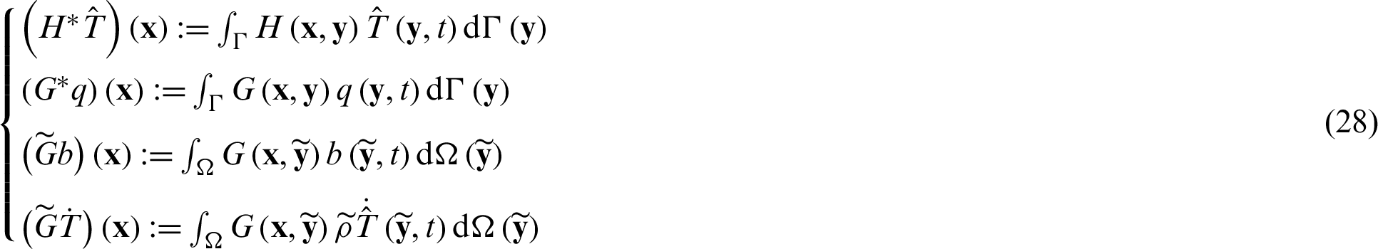
In this work, we do not consider the source. Thus, Eq. (27) can be rewritten as

By observing Eq. (28), we can find that the last term on the right hand of Eq. (30) is domain integral term rather than boundary integral term. In this work, the radial integral method is used to transform domain integral into boundary integral to retain the advantage of dimension reduction of IGABEM.
We firstly approximate unknown temperature gradient  by interpolation calculation. The commonly used interpolation function is radial basis function (RBF). We select a number of collocation points and interpolation to get the approximate formula of variables
  ,
,

where N is the number of collocation points,  is the undetermined coefficient at the i-th collocation point, fi(r) is the radial basis function at the i-th collocation point,
  , and
, and  is the coordinates of the i-th collocation point.
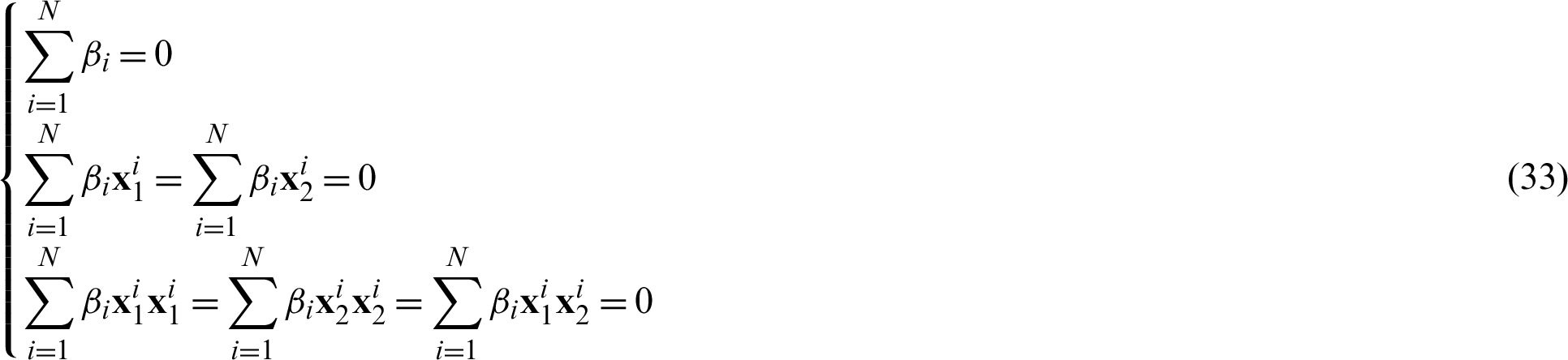
It is worth noting that collocation points can be boundary points or internal points. Generally, combining boundary points and internal points to form collocation points can effectively improve the approximation accuracy. In addition, the accuracy of approximation can be further improved by combining radial basis functions and polynomials, which can be expressed in combination with quadratic polynomials,

where  and
and  are Cartesian coordinate components of the point
  . The following conditions are met:
It is particularly important to determine these coefficients  and
and  in Eq. (32). Although it is not easy to directly express these coefficients, we can get the implicit expression of these coefficients through a series of transformation operations. By setting collocation point as
  in Eq. (32) and assembling them into matrix-vector formulation, we can get the following expression:

where
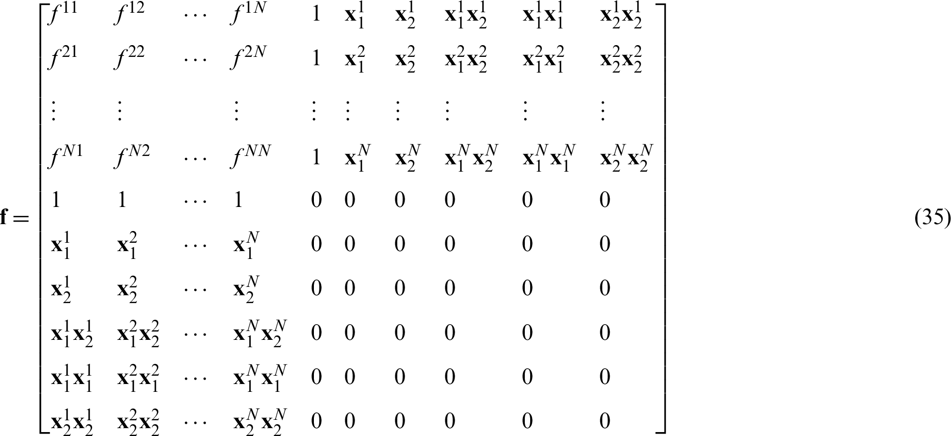
and


where fij = fj(r) in Eq. (35),  , and
, and  denotes the temperature derivative at the i-th collocation point.
When the collocation point is not repeated, the matrix f is invertible. Thus, the coefficient vector v can be expressed as:

By substituting Eq. (33) into the last term on the right of Eq. (27) and using the radial integration method, the following boundary integral formula can be obtained

where
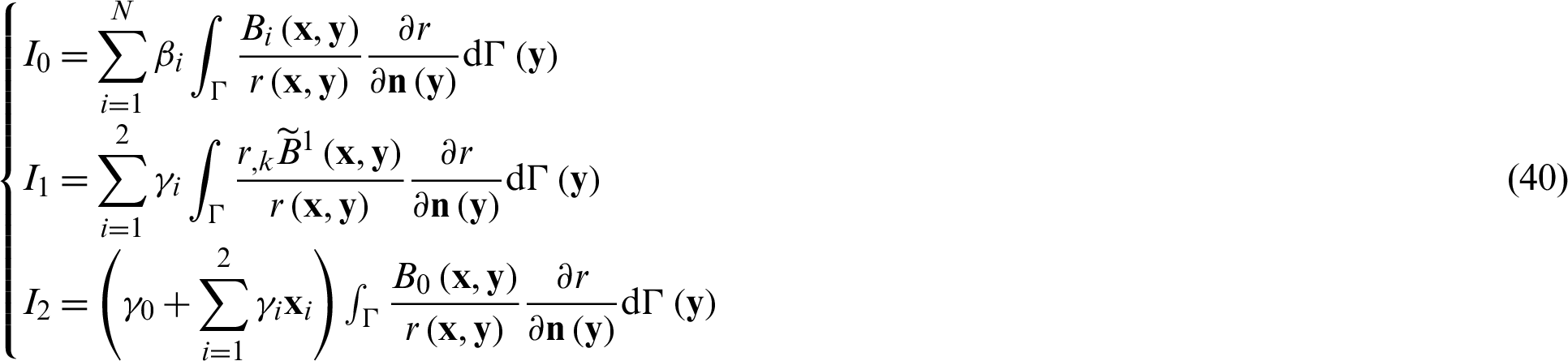
and
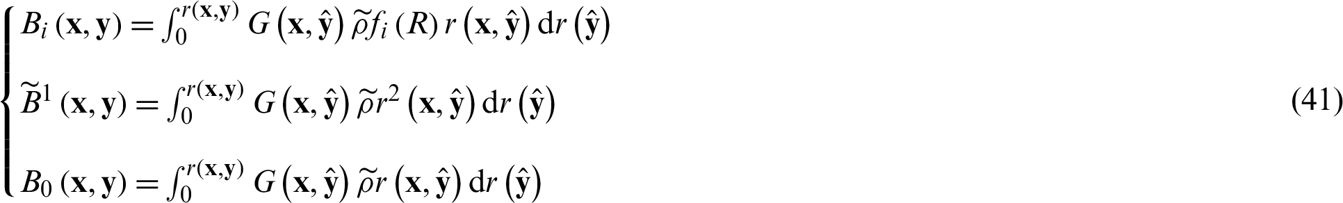
It can be found that the domain integral in Eq. (39) is successfully transformed into the boundary integral. For the detailed derivation process of the above results, also see [42].
It is worth noting that these coefficients in Eq. (40) are unknown, so it is impossible to obtain the results of I0, I1, and I2 directly through the boundary integral calculation. In fact, these coefficients do not need to be calculated directly.
When the source point x is set as the i-th collocation point, the terms I0, I1, and I2 can be rewritten as a formulas of vector and vector multiplication, respectively. By combining the three terms, we can get the following formulas

where the vector  contains the result of the boundary integrals in Eq. (40). By substituting Eq. (38) into Eq. (42), we can obtain the following formulation

where  . When the point x in Eq. (43) is chosen as collocation point, by assembling the equations at all points, we could get a formulation of matrix vector multiplication.
4.2 Discretization of Boundary Integral Equation
First, we discretize the boundary into Ne non-overlapping NURBS elements,

NURBS basis functions are used for approximation. In any NURBS element e, variables can be approximately expressed as follows:
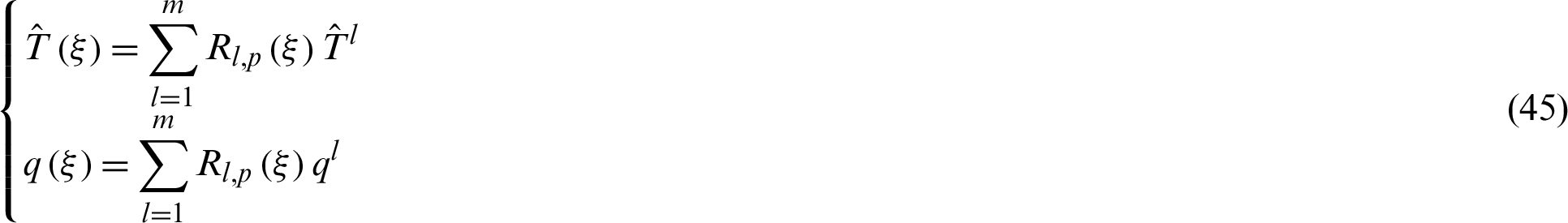
where m is the number of control points,  represents local parametric coordinates,
  and ql are normalized temperature and its flux at the l-th collocation points. In this work, the Greville abscissa is used to define the positions of collocation points in parameter space, also see [39].
By substituting Eq. (45) into Eq. (27), the two boundary integral terms can be rewritten as
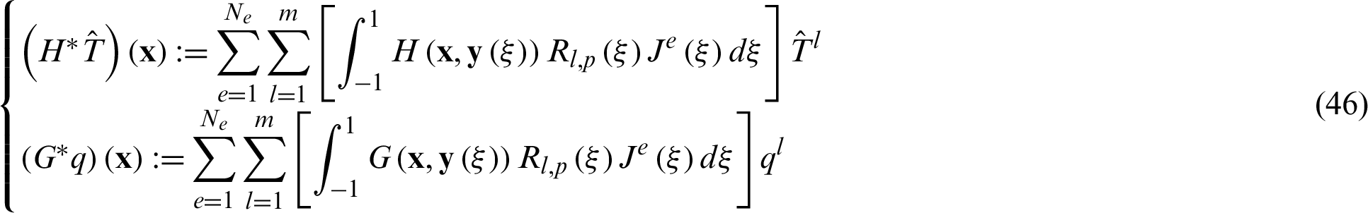
where  denotes Jacobian. Since the last term in Eq. (30) is calculated by radial basis function approximation, only geometric interpolation is needed in the final boundary integrals. Therefore, we only need to replace
  in Eq. (40) with
  . On the other hand, the integrals in the above equations are solved with Gauss integral method. In this work, the number of Gauss quadrature points is set as eight.
After collecting the equations for all collocation points and expressing them in matrix forms, one can obtain the following system of linear algebraic equations:

In this work, the finite difference method is used for solution of the above time domain equations.
It is worth noting that weakly singular integrals exist in Eq. (30). For BEM, it is very important to deal with this kind of singular integral effectively, because it directly determines the accuracy of BEM. Qu et al. [43] and Gong et al. [44] used exponential transformation to calculate accurately the weak singular integrals. Gao et al. [45] used the subtraction of singularity technique to overcome the singularity problem. In this work, the subtraction of singularity technique is also used for calculation of weak singular integrals, see [39].
4.3 Time Marching Method for Solving Transient Heat Conduction Problems
Eq. (27) contains a set of integral equations about time. First, we assume that the total time period is from t0 to tm. And then, divide it into m intervals. Thus, the ith moment can be expressed as:

Herein,  denotes the temperature at ti , and
  denotes the temperature at ti+1 . When the time marching method is used to solve the equations, we can obtain the derivative of temperature with respect to time, as follows:

where the time step  is equal to
  . After interpolation approximation, we can get the temperature
  and its derivative q at
  , as follows:

where  changes from 0 to 1. When
  , it means forward difference scheme is used, when
  , it means backward difference scheme is used, otherwise it means central difference scheme is used. By substituting Eq. (50) into Eq. (30), we can obtain the following formulations

Thus, Eq. (47) can be rewritten as

After merging the similar terms, we can get the following expression:

where

When solving the unknown temperature  or its derivative
  at ti+1, the temperature
  and its derivative
  at ti are all known. Moving all the unknown terms of Eq. (53) to the left-hand side and all the known terms to the right-hand side by considering the boundary conditions, one finally obtain the following system of linear equations:

where B is the coefficient matrix,  is the vector of unknown variable values at the collocation points,
  is the known vector. All the unknown state values can be obtained after Eq. (55) is solved.
Consider a two-dimensional flat plate, the initial temperature is 100 K, the upper and lower boundaries are adiabatic, the left boundary temperature is maintained at 100 K. Convective boundary condition is applied to the right boundary, and the ambient temperature is 400 K, as shown in the Fig. 1. Material density  kg/m3, specific heat capacity cx = 871 J/(kg
 K), thermal conductivity
 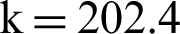 W/(m
W/(m K), convective heat transfer coefficient on the right boundary h = 80 W/(m
 K) and thermal emissivity
  . The boundary element model is as shown in the Fig. 1b. Each boundary is divided into 16 equally spaced linear elements, with a total of 64 boundary elements, 64 boundary nodes and 15 internal points.
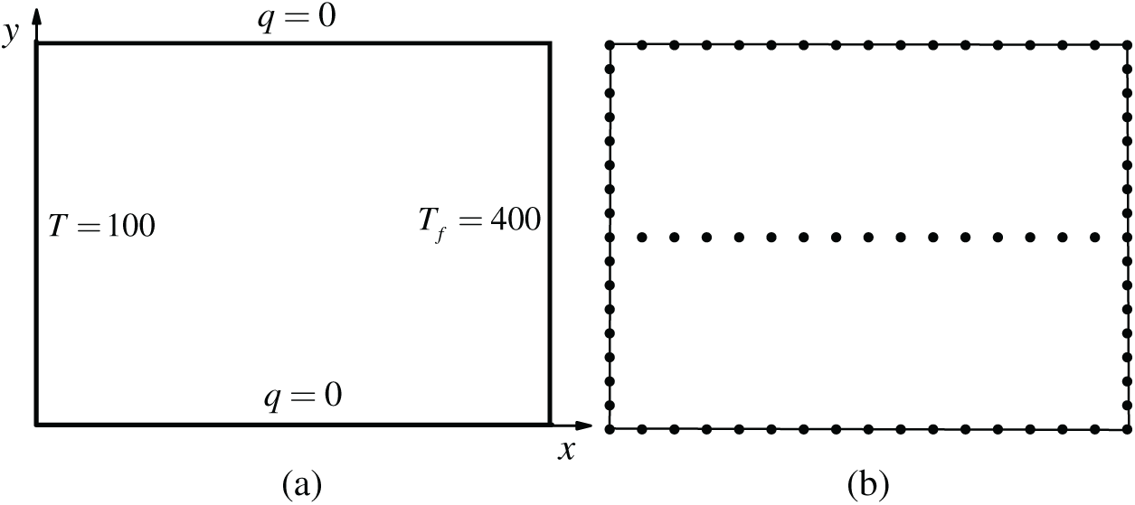
Figure 1: Plate model diagram and boundary conditions. (a) Plate boundary conditions. (b) Plate model diagram
Fig. 2 shows the distribution of temperature along the lower boundary of plate when t = 100, 200, 400 and 600 s. In this figure, the calculation results obtained by using IGABEM are compared with those of the finite volume method (Fluent), and it demonstrates the correctness and validity of this algorithm proposed in this work.
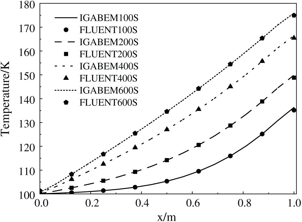
Figure 2: Temperature distribution along the lower boundary of the plate at different times
5.2 An Example of Elliptic Plate
Consider an elliptical plate with a long radius of 2 m and a short radius of 1 m. The initial temperature is 100 K, and the ambient temperature of the plate boundary is 400 K. Material density  kg/m3, specific heat capacity cx = 871 J/(kg
 K), thermal conductivity k = 202.4 W/(m
 K), and boundary convective heat transfer coefficient h = 80 W/(m
 K).
K).
The shape of ellipse and the distribution of internal points are shown in Fig. 3. Fig. 4a shows the initial NURBS curve and the position of control points. After normalizing the knot vector, the parameter space vector of boundary element can be obtained, which is expressed as 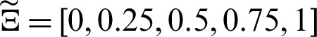 . Therefore, four boundary elements are formed, and the parameter space intervals are [0, 0.25);[0.25, 0.5);[0.5, 0.75);[0.75, 1) respectively. By splitting each NURBS elements equally and inserting new knots, the new control point sequence, knot vector and weight factor vector after refinement can be obtained. For example, insert a new control point on the middle point of each initial NURBS cell parameter space to get the refined control point sequence shown in Fig. 4b, as shown by the black circle point “inserted knots.” After Bézier extraction operation, a new set of control point sequence is obtained, as shown in “BE operation knots.” For “initial knots” in Fig. 4a and “inserted knots” in Fig. 4b, we can find that inserting a new point will also change the position of the original point, but still describe the same curve. However, Bézier extraction operation does not change the position of the original control points, but inserts a new control point at the middle point of some elements. Then, the new control point sequence and Bézier extraction sequence when the initial NURBS cells are divided into 3, 4, 5 and 6 subunits are given in turn, as shown in Figs. 4c–4f respectively.
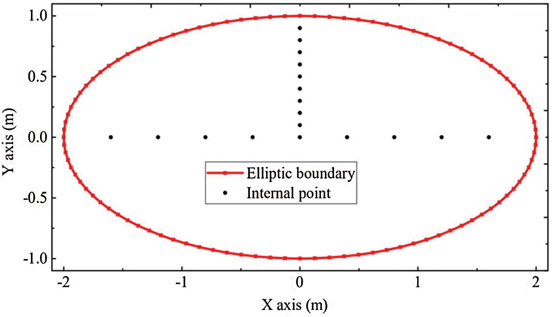
Figure 3: The NURBS curve and internal points for elliptic
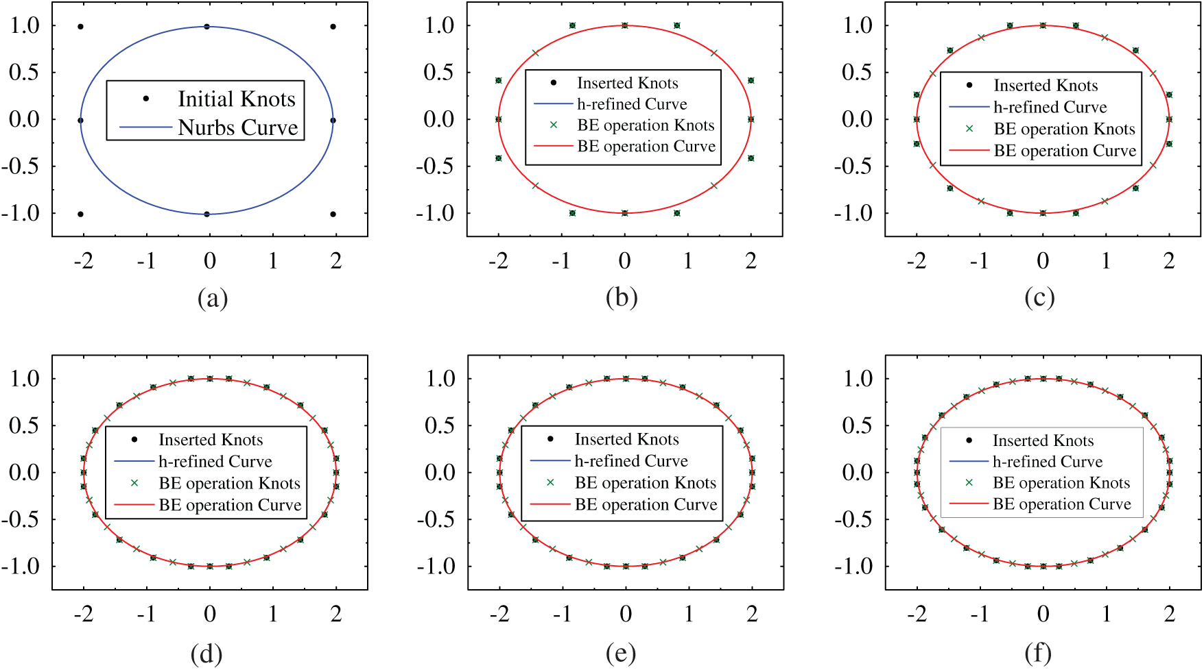
Figure 4: Geometric control points and NURBS curves of elliptical model with different refinement levels. (a) Initial. (b) Refine2. (c) Refine3. (d) Refine4. (e) Refine5. (f) Refine6
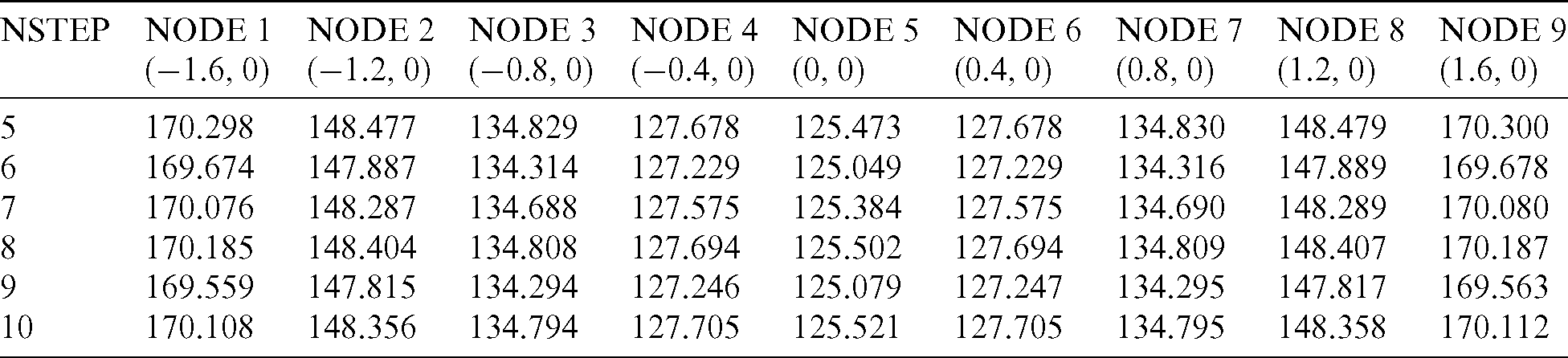
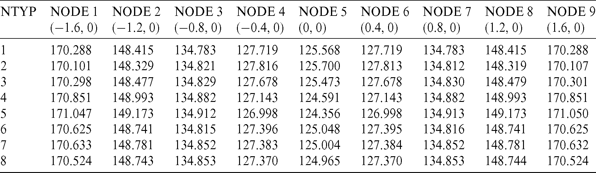
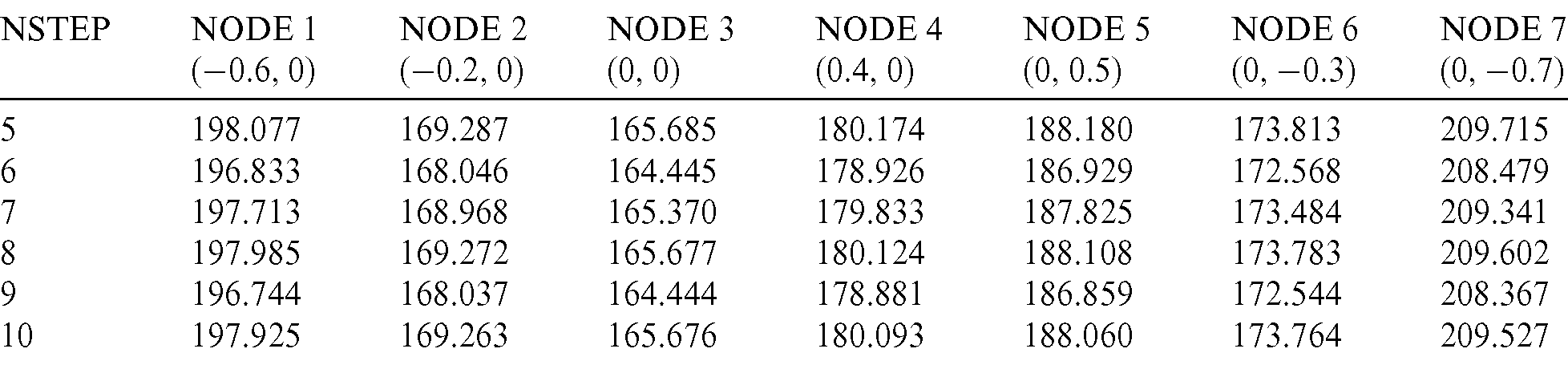
In this work, the finite difference method is used to solve the time-domain equation. Therefore, we first investigate the influence of time step on the calculation results, as shown in Tab. 1. The temperature values at nine points on the x axis are calculated, where different time step is used, for example  , 6, 7, 8, 9, and 10. From this table, we can find that the results with different time steps have small deviation. In fact, too large step value may lead to large error of temperature gradient value, even the calculation is not correct at all. If the time step is too small, it will also lead to inaccurate calculation of temperature gradient value. Therefore, it is very important to select an appropriate time step value. It can be seen from Tabs. 1 and 2 that it is appropriate to set the time step from 5 to 10.
Table 1: Temperature values at several internal points with different time step values in 200 s
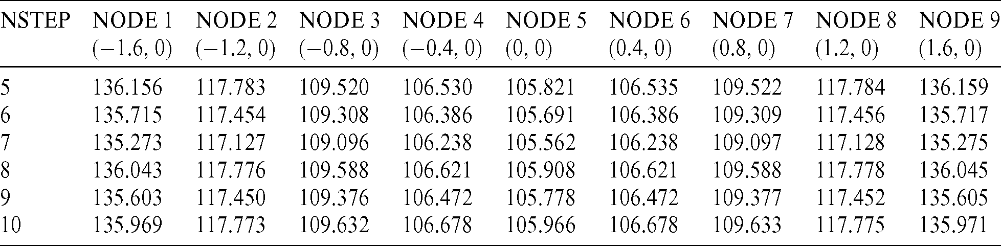
Table 2: Temperature values at several internal points with different time step values in 400 s
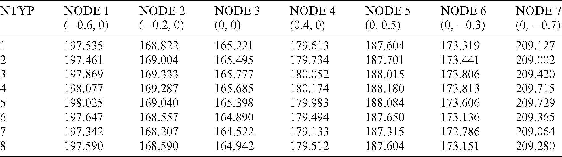
In this work, we use the radial basis method to approximate the temperature gradient. Therefore, it is significant to investigate the influence of different types of radial basis functions on the numerical results. Herein, eight different types of radial basis functions are given, as shown in Tab. 3. Tab. 4 shows the comparison of temperature values at several calculation points when using different radial basis functions, where the time step is 5. By observing Tab. 4, it can be found that the deviation of calculation results in 200 s is very small when using different types of radial basis functions, more results in 400 s are also found in Tab. 5. It verifies the stability of the algorithm proposed.
Table 3: Types of radial basis functions
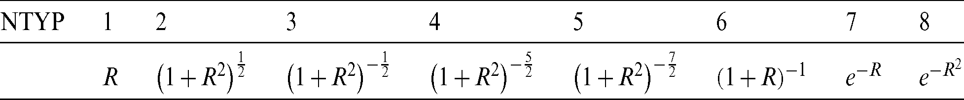
Table 4: Comparison of calculation results with different types of radial basis functions in 200 s
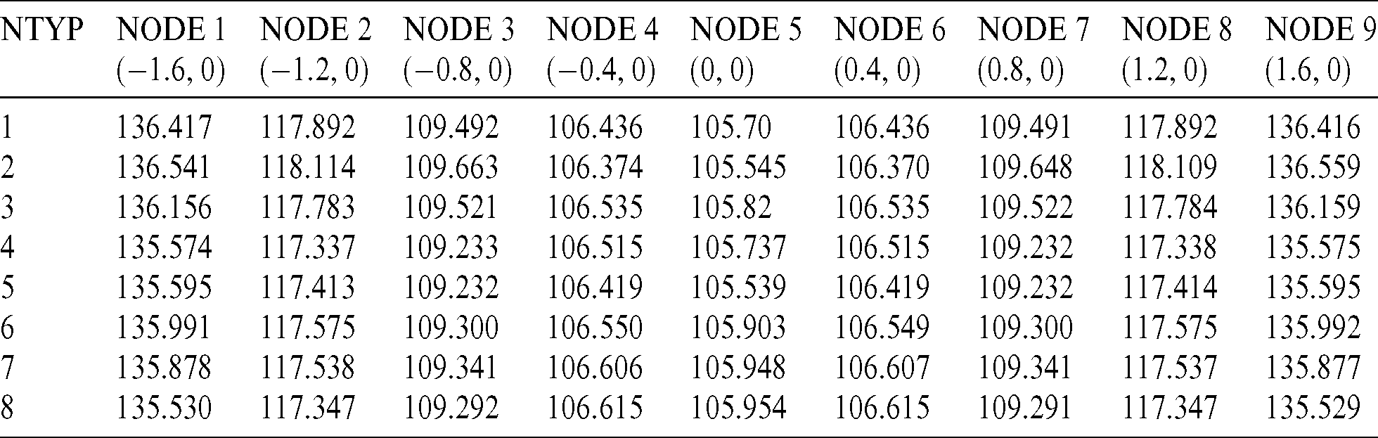
Table 5: Comparison of calculation results with different types of radial basis functions in 400 s
Figs. 5a and 5b respectively show the comparison of temperature values at points on the x axis and y axis based on traditional BEM and IGABEM algorithm developed in this paper. From these two graphs, it can be found that the results of the IGABEM algorithm are consistent with the results of conventional BEM, which verifies the correctness of the algorithm developed in this work.
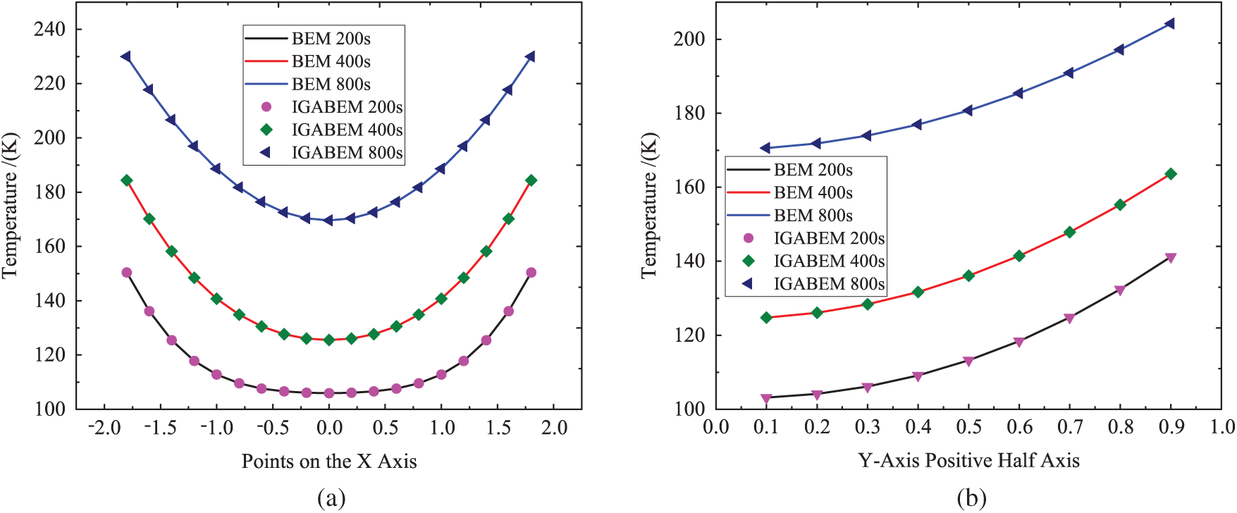
Figure 5: Temperature distribution on X-axis and Y-axis, respectively. (a) Temperature of X-axis symmetry point. (b) Temperature of positive half axis of Y-axis
5.3 An Example of Octagonal Leaf
In this section, we consider an example of octagonal leaf, as shown in Fig. 6. The initial temperature is 100 K, and the ambient temperature of the structural boundary is 600 K. Other physical parameters are consistent with the previous example. The new control point sequence and Bézier extraction sequence when the initial NURBS cells are divided into 2, 3, 4, 5 and 6 subunits are given in turn, as shown in Figs. 7b–7f respectively.
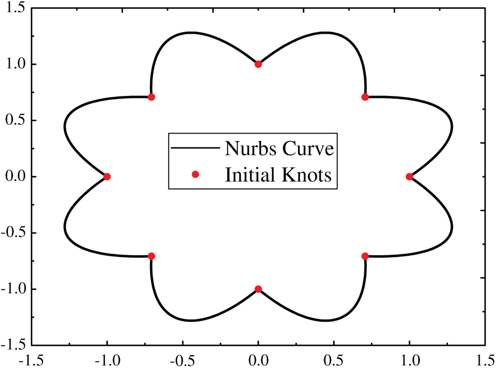
Figure 6: The NURBS curve and internal points for octagonal model
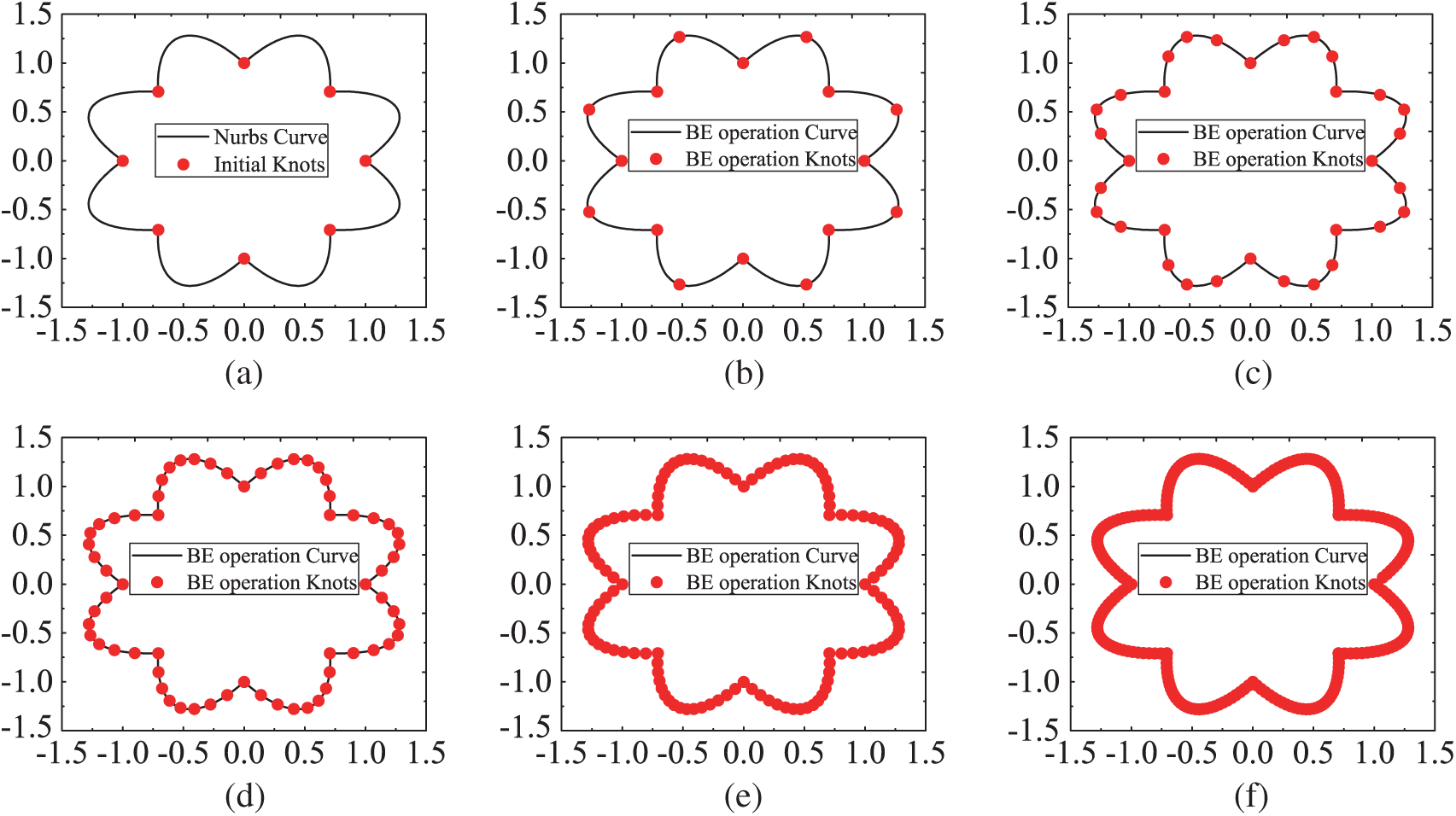
Figure 7: Generation of NURBS curve control points for octagon model. (a) Initial. (b) Refine2. (c) Refine3. (d) Refine4. (e) Refine5. (f) Refine6
Similar to the previous example, we investigate the influence of different radial basis functions on the calculation results, as shown in Tab. 6 for 200 s and in Tab. 7 for 400 s. It shows that there is a small deviation in the calculation results when different radial basis functions are used, which verifies the stability of the algorithm in this work.
Table 6: Comparison of calculation results with different types of radial basis functions in 200 s for octagonal leaf
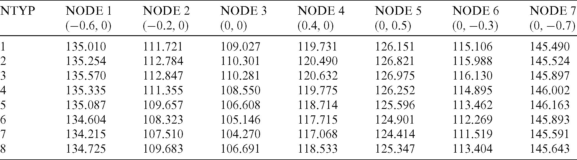
Table 7: Comparison of calculation results with different types of radial basis functions in 400 s for octagonal leaf
The influence of time step parameters on the calculation accuracy can be found in Tab. 8 for 200 s and in Tab. 9 for 400 s. Similar to the previous results, the change of time step parameters from 5 to 10 has little effect on the calculation results, which verifies the stability of the algorithm in this work.
Table 8: Temperature at internal points with different time step values in 200 s for octagonal leaf model
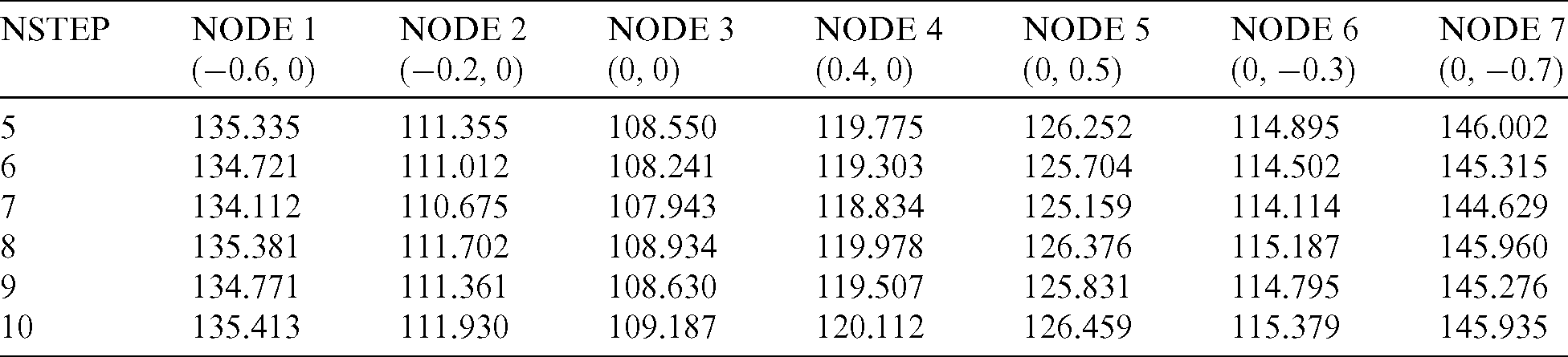
Table 9: Temperature at internal points with different time step values in 400 s for octagonal leaf model
This paper applied IGABEM to the heat conduction problem of temperature field. IGABEM can accurately represent the geometric model. In addition to the advantages of dimensionality reduction, IGABEM can also realize the seamless integration of CAD modeling and numerical analysis. The use of Bézier extraction technique further simplifies the implementation of IGA. This method transformed the basis functions of NURBS into Bernstein polynomials and maintained the consistency of geometric models. The main feature of this method was that the iterative calculation of NURBS basis function was avoided in the process of element physical interpolation calculation of BEM, which can effectively improve the computational efficiency. The domain integral term was successfully converted to the boundary integral in IGABEM with radial integration method. The present method provides a powerful tool for fast and high fidelity simulation of transient heat conduction problems commonly encountered in numerous industrial sectors.
Funding Statement: This research was funded by National Natural Science Foundation of China (NSFC) under Grant Nos. 11702238, 51904202, and 11902212, and Nanhu Scholars Program for Young Scholars of XYNU.
Conflicts of Interest: The authors declare that they have no conflicts of interest to report regarding the present study.
1. Hughes, T. J. R., Cottrell, J. A., Bazilevs, Y. (2005). Isogeometric analysis: CAD, finite elements, NURBS, exact geometry and mesh refinement. Computer Methods in Applied Mechanics and Engineering, 194(39–41), 4135–4195. DOI 10.1016/j.cma.2004.10.008. [Google Scholar] [CrossRef]
2. Cottrell, J. A., Hughes, T. J. R., Reali, A. (2007). Studies of refinement and continuity in isogeometric structural analysis. Computer Methods in Applied Mechanics and Engineering, 196(41–44), 4160–4183. DOI 10.1016/j.cma.2007.04.007. [Google Scholar] [CrossRef]
3. Bazilevs, Y., Michler, C., Calo, V. M., Hughes, T. J. R. (2010). Isogeometric variational multiscale modeling of wall-bounded turbulent flows with weakly enforced boundary conditions on unstretched meshes. Computer Methods in Applied Mechanics and Engineering, 199(13–16), 780–790. DOI 10.1016/j.cma.2008.11.020.
4. Nagy, A. P., Abdalla, M. M., Gürdal, Z. (2010). Isogeometric sizing and shape optimisation of beam structures. Computer Methods in Applied Mechanics and Engineering, 199(17–20), 1216–1230. DOI 10.1016/j.cma.2009.12.010.
5. Benson, D. J., Bazilevs, Y., Hsu, M. C., Hughes, T. J. R. (2010). Isogeometric shell analysis: The Reissner–Mindlin shell. Computer Methods in Applied Mechanics and Engineering, 199(5–8), 276–289. DOI 10.1016/j.cma.2009.05.011.
6. De Lorenzis, L., Temizer, I., Wriggers, P., Zavarise, G. (2011). A large deformation frictional contact formulation using NURBS-based isogeometric analysis. International Journal for Numerical Methods in Engineering, 87(13), 1278–1300. DOI 10.1002/nme.3159. [Google Scholar] [CrossRef]
7. Borden, M. J., Scott, M. A., Evans, J. A., Hughes, T. J. R. (2011). Isogeometric finite element data structures based on Bézier extraction of NURBS. International Journal for Numerical Methods in Engineering, 87(1–5), 15–47. DOI 10.1002/nme.2968. [Google Scholar] [CrossRef]
8. Mierzwiczak, M., Chen, W., Fu, Z. (2015). The singular boundary method for steady-state nonlinear heat conduction problem with temperature-dependent thermal conductivity. International Journal of Heat & Mass Transfer, 91, 205–217. DOI 10.1016/j.ijheatmasstransfer.2015.07.051. [Google Scholar] [CrossRef]
9. Fu, Z. J., Qin, Q. H., Chen, W. (2011). Hybrid-trefftz finite element method for heat conduction in nonlinear functionally graded materials. Engineering Computations, 28(5), 578–599. DOI 10.1108/02644401111141028. [Google Scholar] [CrossRef]
10. Li, T., Gao, Y., Han, D., Yang, F., Yu, B. (2020). A novel POD reduced-order model based on EDFM for steady-state and transient heat transfer in fractured geothermal reservoir. International Journal of Heat and Mass Transfer, 146, 118783. DOI 10.1016/j.ijheatmasstransfer.2019.118783. [Google Scholar] [CrossRef]
11. Wang, Y., Liao, Z., Shi, S., Wang, Z., Hien, Poh L. (2020). Data-driven structural design optimization for petal-shaped auxetics using isogeometric analysis. Computer Modeling in Engineering & Sciences, 122(2), 433–458. DOI 10.32604/cmes.2021.08680. [Google Scholar] [CrossRef]
12. Chen, L., Marburg, S., Chen, H., Zhang, H., Gao, H. (2017). An adjoint operator approach for sensitivity analysis of radiated sound power in fully coupled structural-acoustic systems. Journal of Computational Acoustics, 25(1), 1750003. DOI 10.1142/S0218396X17500035. [Google Scholar] [CrossRef]
13. Banerjee, P. K., Cathie, D. N. (1980). A direct formulation and numerical implementation of the boundary element method for two-dimensional problems of elasto-plasticity. International Journal of Mechanical Sciences, 22(4), 233–245. DOI 10.1016/0020-7403(80)90038-7.
14. Cruse, T. A. (1996). Bie fracture mechanics analysis: 25 years of developments. Computational Mechanics, 18(1), 1–11. DOI 10.1007/BF00384172.
15. Seybert, A. F., Soenarko, B., Rizzo, F. J., Shippy, D. J. (1985). An advanced computational method for radiation and scattering of acoustic waves in three dimensions. Journal of the Acoustical Society of America, 77(2), 362–368. DOI 10.1121/1.391908.
16. Chen, L. L., Zhao, W. C., Liu, C., Chen, H. B., Maburg, S. (2019). Isogeometric fast multipole boundary element method based on burton-miller formulation for 3d acoustic problems. Archives of Acoustics, 44, 475–492.
17. Chen, L., Chen, H., Zheng, C., Marburg, S. (2016). Structural-acoustic sensitivity analysis of radiated sound power using a finite element/discontinuous fast multipole boundary element scheme. International Journal for Numerical Methods in Fluids, 82(12), 858–878. DOI 10.1002/fld.4244.
18. Zhao, W. C., Chen, L. L., Chen, H. B., Marburg, S. (2019). Topology optimization of exterior acoustic-structure interaction systems using the coupled fem-bem method. International Journal for Numerical Methods in Engineering, 119(1), 1–28. DOI 10.1002/nme.6039.
19. Chen, L. L., Zhang, Y., Lian, H., Atroshchenko, E., Ding, C. et al. (2020). Seamless integration of computer-aided geometric modeling and acoustic simulation: Isogeometric boundary element methods based on Catmull-Clark subdivision surfaces. Advances in Engineering Software, 149, 102879. DOI 10.1016/j.advengsoft.2020.102879. [Google Scholar] [CrossRef]
20. Politis, C., Ginnis, A. I., Kaklis, P. D., Belibassakis, K., Feurer, C. (2009). An isogeometric BEM for exterior potential-flow problems in the plane. 2009 SIAM/ACM Joint Conference on Geometric and Physical Modeling, San Francisco, California, USA: ACM. [Google Scholar]
21. Simpson, R. N., Bordas, S. P. A., Trevelyan, J., Rabczuk, T. (2012). A two-dimensional isogeometric boundary element method for elastostatic analysis. Computer Methods in Applied Mechanics and Engineering, 209, 87–100. DOI 10.1016/j.cma.2011.08.008. [Google Scholar] [CrossRef]
22. Simpson, R. N., Bordas, S. P. A., Lian, H., Trevelyan, J. (2013). An isogeometric boundary element method for elastostatic analysis: 2D implementation aspects. Computers & Structures, 118, 2–12. DOI 10.1016/j.compstruc.2012.12.021. [Google Scholar] [CrossRef]
23. An, Z., Yu, T., Bui, T. Q., Wang, C., Trinh, N. A. (2018). Implementation of isogeometric boundary element method for 2-D steady heat transfer analysis. Advances in Engineering Software, 116, 36–49. DOI 10.1016/j.advengsoft.2017.11.008. [Google Scholar] [CrossRef]
24. Scott, M. A., Simpson, R. N., Evans, J. A., Lipton, S., Bordas, S. P. A. et al. (2013). Isogeometric boundary element analysis using unstructured t-splines. Computer Methods in Applied Mechanics and Engineering, 254, 197–221. DOI 10.1016/j.cma.2012.11.001. [Google Scholar] [CrossRef]
25. Li, S., Trevelyan, J., Zhang, W., Wang, D. (2018). Accelerating isogeometric boundary element analysis for 3-dimensional elastostatics problems through black-box fast multipole method with proper generalized decomposition. International Journal for Numerical Methods in Engineering, 114(9), 975–998. DOI 10.1002/nme.5773. [Google Scholar] [CrossRef]
26. Nguyen, B. H., Tran, H. D., Anitescu, C., Zhuang, X., Rabczuk, T. (2016). An isogeometric symmetric galerkin boundary element method for two-dimensional crack problems. Computer Methods in Applied Mechanics and Engineering, 306, 252–275. DOI 10.1016/j.cma.2016.04.002. [Google Scholar] [CrossRef]
27. Peng, X., Atroshchenko, E., Kerfriden, P., Bordas, S. P. A. (2017). Linear elastic fracture simulation directly from CAD: 2D NURBS-based implementation and role of tip enrichment. International Journal of Fracture, 204(1), 55–78. DOI 10.1007/s10704-016-0153-3.
28. Peng, X., Atroshchenko, E., Kerfriden, P., Bordas, S. P. A. (2017). Isogeometric boundary element methods for three dimensional static fracture and fatigue crack growth. Computer Methods in Applied Mechanics and Engineering, 316, 151–185. DOI 10.1016/j.cma.2016.05.038. [Google Scholar] [CrossRef]
29. Simpson, R. N., Liu, Z., Vazquez, R., Evans, J. A. (2018). An isogeometric boundary element method for electromagnetic scattering with compatible B-spline discretizations. Journal of Computational Physics, 362, 264–289. DOI 10.1016/j.jcp.2018.01.025. [Google Scholar] [CrossRef]
30. Simpson, R. N., Scott, M. A., Taus, M., Thomas, D. C., Lian, H. (2014). Acoustic isogeometric boundary element analysis. Computer Methods in Applied Mechanics and Engineering, 269, 265–290. DOI 10.1016/j.cma.2013.10.026. [Google Scholar] [CrossRef]
31. Peake, M. J., Trevelyan, J., Coates, G. (2015). Extended isogeometric boundary element method (XIBEM) for three-dimensional medium-wave acoustic scattering problems. Computer Methods in Applied Mechanics and Engineering, 284, 762–780. DOI 10.1016/j.cma.2014.10.039.
32. Keuchel, S., Hagelstein, N. C., Zaleski, O., von Estorff, O. (2017). Evaluation of hypersingular and nearly singular integrals in the isogeometric boundary element method for acoustics. Computer Methods in Applied Mechanics and Engineering, 325, 488–504. DOI 10.1016/j.cma.2017.07.025.
33. Chen, L., Marburg, S., Zhao, W., Liu, C., Chen, H. (2019). Implementation of isogeometric fast multipole boundary element methods for 2D half-space acoustic scattering problems with absorbing boundary condition. Journal of Theoretical and Computational Acoustics, 27(2), 1850024. DOI 10.1142/S259172851850024X.
34. Chen, L. L., Lian, H., Liu, Z., Chen, H. B., Atroshchenko, E. et al. (2019). Structural shape optimization of three dimensional acoustic problems with isogeometric boundary element methods. Computer Methods in Applied Mechanics and Engineering, 355, 926–951. DOI 10.1016/j.cma.2019.06.012. [Google Scholar] [CrossRef]
35. Chen, L., Liu, C., Zhao, W., Liu, L. (2018). An isogeometric approach of two dimensional acoustic design sensitivity analysis and topology optimization analysis for absorbing material distribution. Computer Methods in Applied Mechanics and Engineering, 336, 507–532. DOI 10.1016/j.cma.2018.03.025. [Google Scholar] [CrossRef]
36. Li, K., Qian, X. (2011). Isogeometric analysis and shape optimization via boundary integral. Computer-Aided Design, 43(11), 1427–1437. DOI 10.1016/j.cad.2011.08.031. [Google Scholar] [CrossRef]
37. Lian, H., Kerfriden, P., Bordas, S. P. A. (2016). Implementation of regularized isogeometric boundary element methods for gradient-based shape optimization in two-dimensional linear elasticity. International Journal for Numerical Methods in Engineering, 106(12), 972–1017. DOI 10.1002/nme.5149.
38. Lian, H., Kerfriden, P., Bordas, S. P. A. (2017). Shape optimization directly from CAD: An isogeometric boundary element approach using T-splines. Computer Methods in Applied Mechanics and Engineering, 317, 1–41. DOI 10.1016/j.cma.2016.11.012.
39. Liu, C., Chen, L., Zhao, W., Chen, H. (2017). Shape optimization of sound barrier using an isogeometric fast multipole boundary element method in two dimensions. Engineering Analysis with Boundary Elements, 85, 142–157. DOI 10.1016/j.enganabound.2017.09.009. [Google Scholar] [CrossRef]
40. Chen, L., Lu, C., Lian, H., Liu, Z., Zhao, W. et al. (2020). Acoustic topology optimization of sound absorbing materials directly from subdivision surfaces with isogeometric boundary element methods. Computer Methods in Applied Mechanics and Engineering, 362, 112806. DOI 10.1016/j.cma.2019.112806. [Google Scholar] [CrossRef]
41. Gao, X. W. (2002). The radial integration method for evaluation of domain integrals with boundary-only discretization. Engineering Analysis with Boundary Elements, 26(10), 905–916. DOI 10.1016/S0955-7997(02)00039-5. [Google Scholar] [CrossRef]
42. Gao, X. W., Peng, H. F. K. Y. J. W. (2015). Theory and program of advanced boundary element method. Beijing, China: Science Press. [Google Scholar]
43. Qu, X. Y., Dong, C. Y., Bai, Y., Gong, Y. P. (2018). Isogeometric boundary element method for calculating effective property of steady state thermal conduction in 2D heterogeneities with a homogeneous interphase. Journal of Computational and Applied Mathematics, 343, 124–138. DOI 10.1016/j.cam.2018.04.053. [Google Scholar] [CrossRef]
44. Gong, Y., Trevelyan, J., Hattori, G., Dong, C. (2018). Hybrid nearly singular integration for isogeometric boundary element analysis of coatings and other thin 2D structures. Computer Methods in Applied Mechanics and Engineering, 346, 642–673. DOI 10.1016/j.cma.2018.12.019. [Google Scholar] [CrossRef]
45. Gao, X., Trevor, G. D. (2002). Boundary element programming in mechanics. Cambridge, UK: Cambridge University Press. [Google Scholar]
 | This work is licensed under a Creative Commons Attribution 4.0 International License, which permits unrestricted use, distribution, and reproduction in any medium, provided the original work is properly cited. |