Computer Modeling in Engineering & Sciences

DOI: 10.32604/cmes.2021.011857

ARTICLE

Development of TD-BEM Formulation for Dynamic Analysis for Twin-Parallel Circular Tunnels in an Elastic Semi-Infinite Medium

Weidong Lei1, Hai Zhou1,*, Hongjun Li2 and Rui Chen1

1School of Civil and Environmental Engineering, Harbin Institute of Technology, Shenzhen, 518055, China
2Urban and Rural Construction Institute, Hebei Agricultural University, Baoding, 071001, China
*Corresponding Author: Hai Zhou. Email: zhouhai@stu.hit.edu.cn
Received: 02 June 2020; Accepted: 19 October 2020

1  Introduction

Due to the demanding development and the limited space in urban areas, complex underground structures including the parallel subway tunnels, spaced at a limited distance, are being constructed. Although the subway brings convenience, a moving vehicle on uneven rails produces a dynamic force between wheels and rails and causes vibration, which has potential negative effects on sub-infrastructure beneath the rails, twin-parallel tunnels and even the structures on the ground [1,2].

Without loss of generality, taking the unballasted track in a subway project as an example, the whole propagation process of subway vibration could be roughly divided into two phases: First, the coupled vibration between rails and the wheels of the vehicle acts on the track slab, sequentially passes through the CA mortar layer, the railway ballast, the lining of the tunnel and the outer protective layer of the lining. And after that, the vibration propagates in the semi-infinite surrounding rocks or soils. Since the layout of the parallel subway tunnels is generally in the form of long cylinders in semi-infinite rocks or soils, the subway vibration analysis system could be illustrated by a plane model, as shown in Fig. 1.

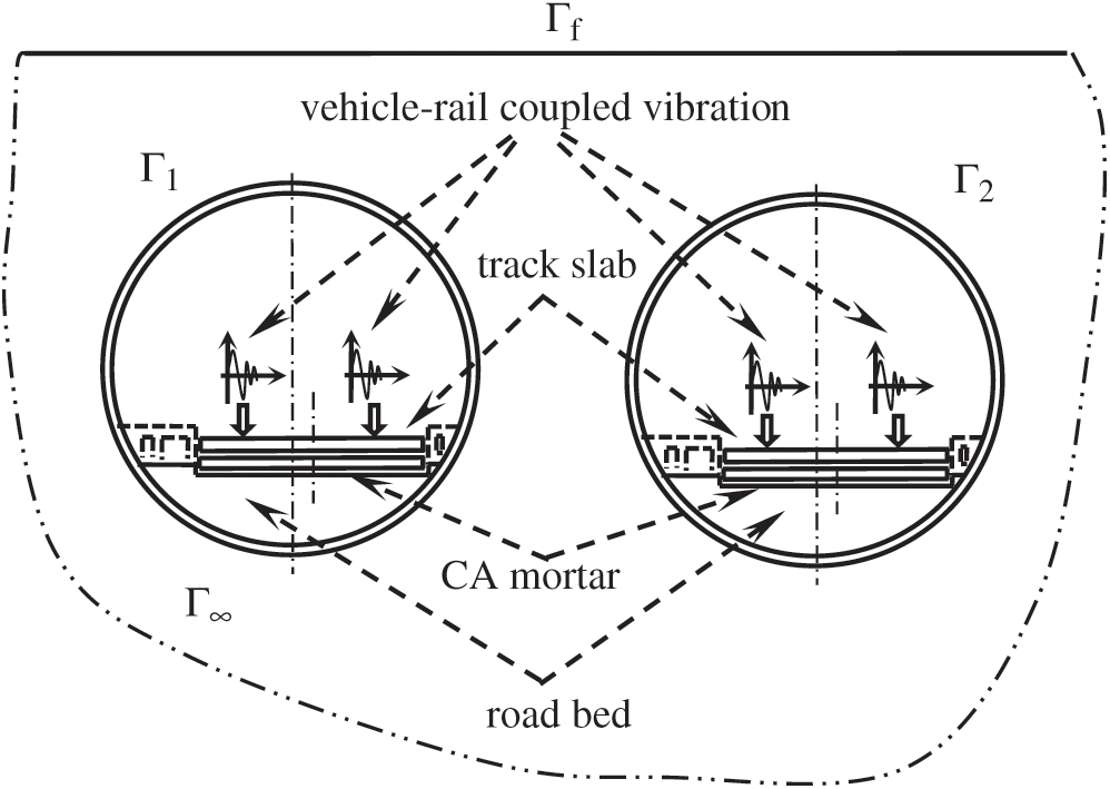
Figure 1: 2-D vibration analysis model

In order to fully understand the propagation law of subway vibration, great efforts have been devoted to developing numerical models for the dynamic track-tunnel-soil system, among which finite element method (FEM) is widely used. However, FEM requires an artificial boundary when dealing with infinite or semi-infinite problems, so it is not the ideal numerical tool. Since boundary element method (BEM) is good at simulating the radiational wave propagation in semi-infinite soils, the FEM–BEM coupled model would be most attractive [3–5]. Usually, FEM should be employed to dynamically simulate the track-tunnel system, where vibration forces in the boundary of the tunnel due to the passage of a train could be determined. Then, BEM should be introduced to model the dynamic response of the surrounding soil.

In comparison with FEM, BEM has irreplaceable advantages in dealing with infinite or semi-infinite problems, automatically satisfying Sommerfeld’s radiation conditions at the infinity for infinite and semi-infinite domains, restricting the discretization only on the boundary of the computational domain for elastic analysis [6–10]. Besides, reducing the dimensionality for the problem and possessing good computational accuracy are its other advantages [11–13].

BEM for elastodynamic problems could be classified according to the nature of the adopted fundamental solutions [14]. The time domain boundary element method (TD-BEM) employs time dependent fundamental solutions [15], Laplace transform method adopts the Laplace transform of the fundamental solutions [16] and the dual reciprocity method (DR-BEM) uses the fundamental solutions of elastostatics [17]. It is obvious that TD-BEM provides a direct way of obtaining the time history of the response for transient problems without any domain transforms [18]. The use of time domain fundamental solutions turns TD-BEM formulation very elegant and attractive from the mathematical point of view [14,15,18]. In addition, the fulfillment of the radiation condition by time domain fundamental solutions turns the formulation suitable for performing infinite domain analysis, since there are no reflected waves from the infinity [19,20].

TD-BEM formulation for elastodynamics was originally proposed for the first time in two journal papers by Mansur et al. [21,22] and after that in Mansur’s Ph.D thesis [23]. Subsequently, Carrer et al. [24,25] found the procedure to work out the integral equation for stresses at internal points, where kernels were calculated by adopting the concept of the finite part of an integral, rather than following the kernel regularization procedure presented by Mansur [21–23]. Based on the above researches, extensive studies on applying and improving TD-BEM formulation for elastodynamic problems were conducted. Zhang [26] applied TD-BEM for transient elastodynamic crack analysis, and he and his colleagues [27] developed the numerical scheme in orthotropic media. Alielahi et al. [28] used TD-BEM to study the seismic ground response in the vicinity of an embedded circular cavity. Lei et al. [29] presented the analytical treatment to the singular integral terms in boundary integral equations, which improved the computation accuracy of TD-BEM for 2-D elastodynamic problems. Several other studies [30–33] were devoted to improving computational stability.

The above mentioned studies are focused mainly on infinite domain problems, where only the discretization on the boundary is required and external boundaries are not required to be artificially truncated. However, many practical geotechnical engineering problems require models associated with the semi-infinite domain. The stress free conditions on the ground surface should be taken into consideration when dealing with semi-infinite problems by TD-BEM [34]. Three approaches were proposed for the analysis of the problem with the semi-infinite medium. The first approach is to find semi-infinite fundamental solutions [35,36], where the stress free conditions are automatically satisfied and the discretization of the boundary of the ground surface is not required. However, semi-infinite fundamental solutions are obtained with the assistance of the method of source image, which means that the smooth and regular ground surface is a must. The second approach is to artificially truncate the boundary of the ground surface to the bounded region of the manageable size [37]. Therefore, it increases the degree of freedom and the amount of calculation to obtain acceptable results. The other approach is to incorporate the infinite boundary element into the boundary element analysis [38,39], making full use of the simplicity of full plane fundamental solutions and decreasing the discretization of the free surface. Therefore, the last method is the most effective, compared with the other two methods.

The idea of the infinite boundary element and the reciprocal decaying shape function were first proposed by Watson [40], and after that, Zhang et al. [41] incorporated the infinite boundary element in BEM formulation and applied the formulation to the static problem of a dam foundation. Davies et al. [42] developed the semi analytical approach based on the circular region of exclusion in the far field and described the order adaptive criteria for the numerical integrations. The algorithm was further improved in the subsequent paper [43] by means of the analytical integration of the strongly singular traction kernel. All the aforementioned works are valuable efforts to try to incorporate the infinite boundary element in BEM formulation for elastostatic problems. Unfortunately, to the authors’ best knowledge, the TD-BEM formulation, which incorporates the infinite boundary element to deal with dynamic problems, has not been reported in current references.

By removing the FEM sub-model in the ideal FEM–BEM coupled model in Fig. 1 for the propagation of the vehicle-rail coupled vibration in the semi-infinite soils or rocks, the remaining model becomes the BEM sub-model, as shown in Fig. 2. Therefore, the development of TD-BEM formulation for dynamic analysis of twin tunnels under dynamic loads in an elastic semi-infinite medium is one of the key points in the ideal FEM–BEM coupled model for the dynamic track-tunnel-soil system.

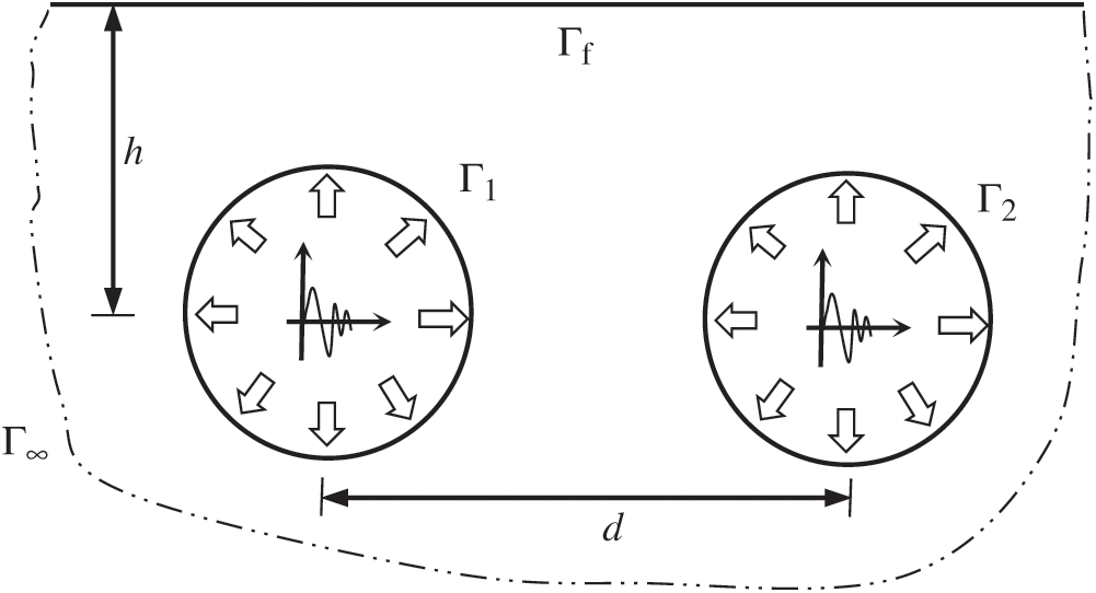
Figure 2: TD-BEM model in the vibration analysis system

This paper presents the semi-infinite TD-BEM formulation for analyzing the dynamic response of twin-paralleled circular tunnels under dynamic loads. Time domain boundary integral equations for this problem are presented, and then, the numerical implementation by introducing the infinite boundary element is presented. Finally, the presented TD-BEM formulation for twin-parallel tunnels in an elastic semi-infinite medium, in which the infinite boundary element and time domain fundamental solutions are incorporated, is verified by a deliberately designed example.

2  Boundary Integral Equations in an Elastic Semi-Infinite Medium

2.1 Displacement Boundary Integral Equation

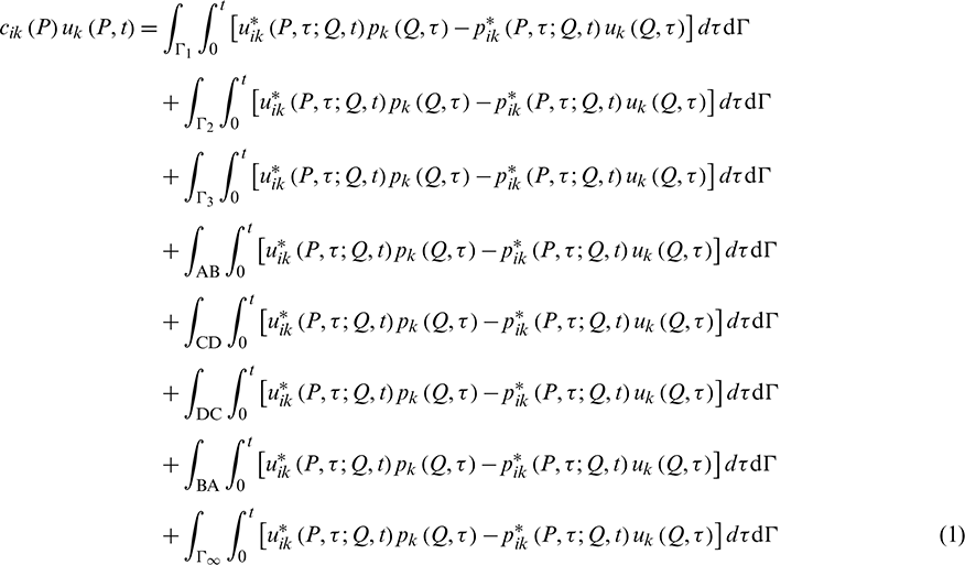
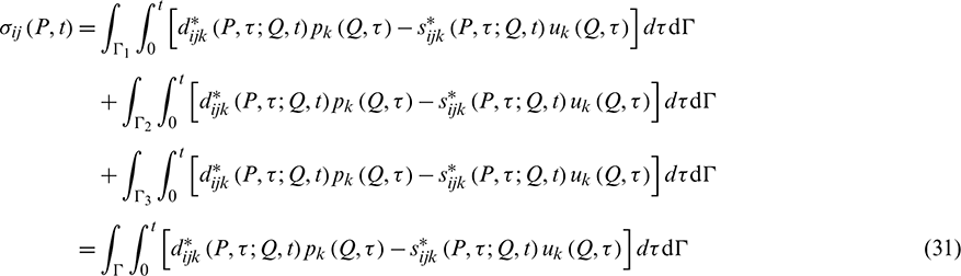
The boundaries for the semi-infinite domain problem include finite boundaries and , the boundary of ground surface and nominal boundaries at the infinity , as shown in Fig. 3. By referring to [35], the displacement boundary integral equation for the elastic, isotropic and homogeneous semi-infinite domain containing twin-parallel circular tunnels based on Betti’s reciprocal work theorem, ignoring contributions from initial conditions and body forces, can be expressed as:

where is a parameter that depends on the position of the source point P; and are displacement and traction components in the k direction, respectively; 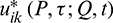and 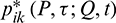stand for time domain displacement and traction fundamental solutions respectively, representing the displacement and traction at the field point Q in the k direction at t instant due to a unit point force applied at the source point P in the i direction at any time instant .

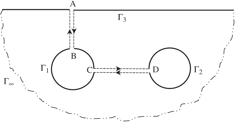
Figure 3: Schematic diagram of the semi-infinite domain with twin-parallel tunnels

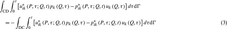
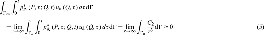
It is noted that the boundaries AB, BA, CD, and DC are virtual boundaries, and their relations are shown in Eqs. (2) and (3). The infinite terms in Eq. (1) can be simplified in Eqs. (4) and (5).

Thus, the displacement boundary integral equation can be re-formulated, as:

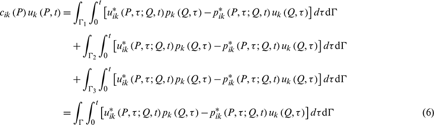
where .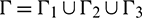

The displacement and traction fundamental solutions in Eq. (6) can be formulated by Eqs. (7) and (8), according to [24,29]:

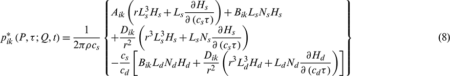
The corresponding integrals of fundamental solutions are expressed by Eqs. (9) and (10):

In Eqs. (9) and (10), is the density, and r is the distance between the field point Q and the source point P. cs is the shear wave velocity or S wave velocity, and cd is the compression wave velocity or P wave velocity. These parameters are expressed as follows:

where

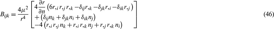
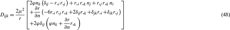
The tensors Eik, Fik and Jik (in Eq. (9)) and Aik, Bik and Dik (in Eq. (10)), which are related only to space, are defined by:

where

The parameters that are relevant to both space and time in the Eqs. (9) and (10) are expressed, as:

where is the Heaviside step function, such that:

It should be noted that the subscript w could be substituted with s or d in the Eqs. (26)–(28), representing the contribution of the shear wave (S wave) or the compression wave (P wave), respectively.

In Eq. (10), the symbol represents the finite part of the integral. Interested readers could refer to references [24,29,44] for more details about the concept and the applications of the finite part of an integral. According to references [24,44], the first term in the bracket in Eq. (10) is used as an example to explain how the finite part of the integral is calculated, as:

In the following context, all the finite parts of the singular integrals are analogously calculated.

2.2 Stress Integral Equation

The stress integral equation for internal points is obtained by combining Hooke’s law with the derivatives of Eq. (6), which is expressed, as:

where

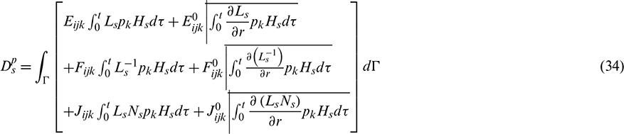
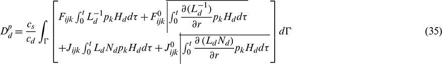
In references [24,25], the stresses at surface nodes are computed using simple finite difference formulae, which employ the displacements and tractions computed by the TD-BEM formulation. The stress integral equation at internal points is expressed, as:

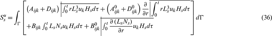
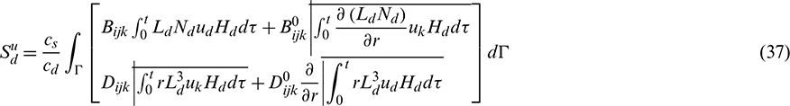
where and represent the contribution of shear and compression waves to the integrals related to the tractions and displacements, respectively. According to references [24,25,29], the terms are expressed in Eqs. (34)–(37):

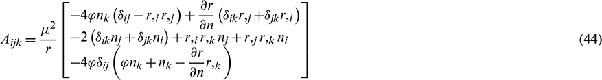
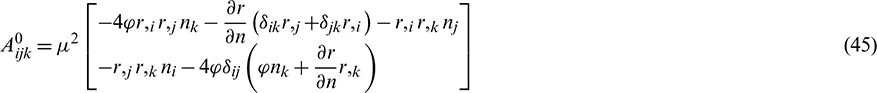
The tensors Eijk, Fijk, Jijk, , and (in Eqs. (34) and (35)) and Aijk, Bijk, Dijk, , and (in Eqs. (36) and (37)), which are related to space, are expressed, as:

By recalling the expressions, Eqs. (11)–(30), these tensors can be calculated, and the boundary integral equation in terms of the internal stress Eq. (31) is determined.

3  Numerical Implementation

3.1 Temporal Discretization

The displacement is assumed to have the linear variation in time, whereas the traction is assumed to be constant. For the given time interval [tm −1, tm], the variables of the displacement and the traction can be written:

where the time interpolation functions are defined, as:

3.2 Spatial Discretization

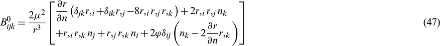
Fig. 4 shows the boundary discretization and the distribution of boundary elements for twin-parallel tunnels in a semi-infinite domain, including infinite boundary elements. The finite boundaries, and , are linear boundary elements. Quadratic boundary elements are adopted to describe infinite boundary elements in spatial discretization.

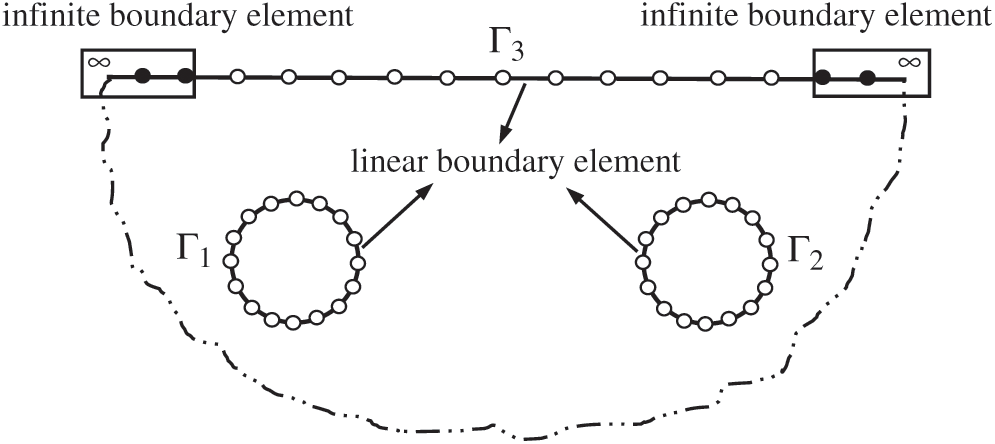
Figure 4: Schematic diagram of boundary discretization

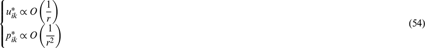
From the expressions of fundamental solutions, Eqs. (7) and (8), it can be seen that and are the same orders as the functions of 1/r and 1/r2, respectively. When r approaches , meaning that the field point Q tends to the infinity, and are the infinite small functions with the same orders as the functions of 1/r and 1/r2, which could be mathematically expressed, as:

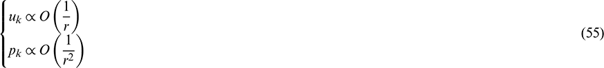
The displacement solution and traction solution can be obtained by the superpositions of displacement and traction fundamental solutions respectively, so decay rates of and also possess the same orders as the functions of 1/r and 1/r2, respectively, when the field point Q tends to the infinity, as:

Therefore, besides the satisfaction of the convergence criterion, the interpolation mode of the infinite boundary element needs to reflect the above mentioned decaying characteristics at the infinity. The requirements about the shape functions of infinite boundary elements are

  i)  Delta function property,

 ii)  Completeness,

iii)  When the field point Q is at the infinity, , ,

There are left and right forms for the infinite boundary elements, as shown in Fig. 5. The shape functions of the displacement and traction for infinite boundary elements are respectively expressed in Eqs. (56) and (57).

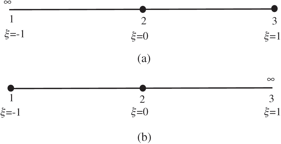
Figure 5: Infinite boundary elements models (a) left (b) right

It is obvious that the above shape functions possess delta function property and completeness. Moreover, when approaches −1 in the left infinite boundary element, meaning that the field point Q tends to the infinity, the displacement solution and the traction solution have the following relations:

For the right infinite boundary element, these relations are also applicable when approaches 1. It has been proved that the above shape functions meet the above requirements for infinite boundary elements.

It is also noted that the stress on the ground surface is free, i.e., is null. One has,

The linear interpolation functions of the displacement and the traction in space can be expressed as:

Therefore, the variables of the displacement and the traction after discretization in both time and space can be rewritten as:

where Nq represents the number of nodes in the boundary element.

So far, according to the decaying characteristics of fundamental solutions from the finite boundary to the infinity, the shape functions for infinite boundary elements are constructed to mathematically describe the relationships between the infinite boundary and the infinity for the field variables. Moreover, the shape functions satisfy the convergence criterion.

3.3 Discretization of Boundary Integral Equations

The numerical solutions to Eqs. (6) and (31) are obtained after discretization both in space and time. The boundaries are discretized into N boundary elements, and the time interval of the analysis [0, t] is divided into M time intervals, each with the same length . The terms of the displacement and the traction in boundary integral equations are respectively expressed as follows:

In Eq. (63), the coefficients and respectively describe the influences of the traction and displacement at node a of element e at instant mt on the displacement of the source point. In Eq. (64), the coefficients and describe the influences of the traction and displacement at node a of element e at instant mt on the stress of the source point.

The values of influencing coefficients are calculated by using the effective method in [29], where the analytical treatments of the singular integral terms were presented, and to which the interested readers could refer for details.

3.4 Matrix form of Boundary Integral Equations

The influencing coefficients at node a of element e at instant are assembled based on one-to-one correspondence in time and space. After that, boundary integral equations are expressed in matrix forms, and the programs of the TD-BEM formulation could be coded.

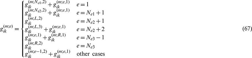
The influencing coefficients of the displacement at node a of element e at instant are obtained by adding the influencing coefficients caused by the (m + 1)th time step and those caused by the mth time step, as shown in Eqs. (65) and (66)

where the superscripts 1 and 2 respectively refer to the forward temporal node in the (m + 1)th time step and the backward temporal node in the (m)th time step.

To further simplify, the influencing coefficients of linear spatial elements are also assembled. The influencing coefficients of element e are obtained by adding the influencing coefficients at the first node of element e and those at the second node of element (e −1). The specific assemblage equations are expressed as follows:

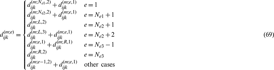
where Nei (i = 1, 2, 3) represents the total number of elements for the corresponding boundaries , and .

When the source point P traverses all boundary nodes, the matrix forms of boundary integral equations after the assemblage can be expressed as follows:

where

In Eq. (71), and denote the displacement and traction vectors at instant respectively, and matrix is constituted by the coefficient. and are boundary influence matrices corresponding to the coefficients and respectively. In Eq. (72), is the vector representing the stress components at instant , and matrices and are correspondingly constructed by coefficients and respectively.

4  Numerical Verification and Discussion

This section is to verify the applicability and the accuracy of the presented TD-BEM formulation for twin-parallel tunnels in an elastic semi-infinite medium, where the infinite boundary elements are incorporated and the time domain fundamental solutions are adopted.

For the purpose of verifying the algorithm, the example with analytical solutions should be the best, because of the uniqueness and the objectivity of the analytical solution. Unfortunately or fortunately, although the analytical solution to the response of the twin-parallel tunnels under dynamic load in an elastic semi-infinite medium is not available, the analytical solution to the response of the single tunnel under dynamic load in an elastic infinite medium is available. Therefore, the numerical example for twin-parallel tunnels is deliberately designed to utilize the analytical solution to the response of the single tunnel under dynamic load in an elastic infinite medium to verify the presented TD-BEM formulation for twin-parallel tunnels under dynamic load in an elastic semi-infinite medium. As shown in Fig. 6a, two parallel circular subway tunnels (r0 = 3 m) are deliberately assumed to be buried in enough deep depth (h = 30 m) beneath the ground surface and are spaced at enough faraway distance (d = 120 m). Monitoring point A is positioned at a nearer distance (6 m) to the center of the left circular tunnel than to the right. The twin-parallel tunnels are assumed to be subjected to the same Heaviside uniform loads p = 200 MPa, shown in Fig. 6b, suddenly at the same time. The mechanical parameters of the surrounding soil are: the elastic modulus Pa, Poisson ratio and the density kg/m3.

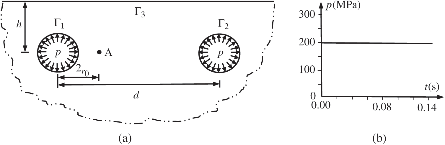
Figure 6: Sketch of the example (a) geometry of tunnels and distribution of loads and (b) load definition

In this scenario, theoretically, the response of monitoring point A could be classified into the early phase and the late phase. In the early phase, the wave initiated from the left tunnel has arrived at and passed by point A, while the reflected wave from the ground, due to the wave from the left tunnel, has not yet arrived, let alone the more faraway wave from the right tunnel. In the late phase, the wave at monitoring point A is subsequently disturbed by the reflected wave from the ground and by the propagating wave from the right tunnel. Therefore, the response of monitoring point A for the problem of twin-parallel tunnels in half-plane in the early phase should be the same as the response of the problem of a single circular tunnel in an infinite medium. According to the analytical wave velocity ( m/s) in the surrounding ideal elastic soil, the early phase is from 0.000 s to 0.029 s, and the late phase is from the instant of the occurrence of the disturbance of the reflected wave from the ground at the instant of 0.029 s to the instant of the analysis, during which the additional disturbance of the wave from the right tunnel joins at the instant of 0.055 s. Therefore, the response of monitoring point A in the early phase for the problem of twin-parallel circular tunnels in the semi-infinite medium from the presented TD-BEM could be compared with the analytical response from the method of characteristics for the problem of the single circular cavity under dynamic load in an infinite medium given by Chou et al. [45] to verify the presented TD-BEM formulation. It is noted that the analytical solution of the single circular cavity in an infinite medium in [45] has been used to verify the TD-BEM formulation in several references [24,29], to which the interested readers could refer for more information and mutual comparison.

Figs. 7a–7c show the comparison between the calculated results from the presented TD-BEM for the problem of twin-parallel circular tunnels in an elastic semi-infinite medium and from the method of characteristics for the problem of single circular cavity in an infinite medium in terms of radial stress (), circumferential stress () and velocity (vr) respectively at monitoring point A.

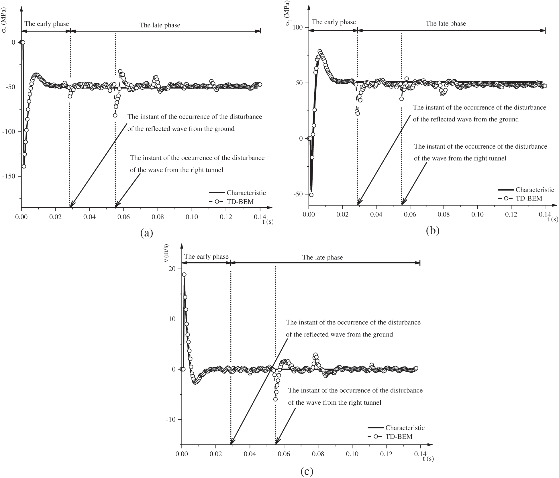
Figure 7: Comparison between results at point A (2ro, 0). (a) Radial stress . (b) Circumferential stress . (c) Velocity vr

From Figs. 7a–7c, it can be seen that, in the early phase (0.000–0.029 s), good agreement between calculated results from the presented TD-BEM and those from the method of characteristics is obtained. This observation quantitively invalidates the applicability and accuracy for the presented TD-BEM formulation for twin-parallel circular tunnels in an elastic semi-infinite medium in the early phase. It can also be seen from the figures that, in the late phase (0.029–0.14 s), the calculated results from the presented TD-BEM fluctuate around the analytical results from the method of the characteristics, with dramatic differences in general in the whole late phase and with sudden changes at the occurrence of the disturbance of the reflected wave from the ground surface and at the occurrence of the additional disturbance of the wave from the right tunnel, indicating the effects of the reflected wave and the interaction of the waves. Meanwhile, good agreement between the calculated instants of the occurrences of the disturbances from the presented TD-BEM and the corresponding analytical instants are obtained. These two observations qualitatively invalidate the applicability and accuracy for the presented TD-BEM formulation for twin-parallel circular tunnels in an elastic semi-infinite medium in the late phase.

5  Conclusions

This study is concerned with developing TD-BEM formulation for dynamic analysis for twin-parallel circular tunnels in a semi-infinite medium, with the following conclusions:

•    Time domain fundamental solutions are adopted in the boundary integral equations in TD-BEM formulation for twin-parallel tunnels under dynamic loads in an elastic semi-infinite medium. The time domain fundamental solutions make it possible to directly and effectively obtain the time history of the response in the presented TD-BEM formulation.

•    In the process of the numerical implementation, infinite boundary elements are incorporated in TD-BEM formulation to satisfy the stress free conditions on the ground surface, moreover, to reduce the discretization of the boundary of the ground surface.

•    The applicability and the accuracy of the TD-BEM formulation are verified by comparing the calculated results from the presented TD-BEM with those from the method of characteristics in the deliberately designed example.

•    The presented TD-BEM formulation could be a step forward in the ideal FEM-BEM coupled model for twin-parallel tunnels under dynamic loads in an elastic semi-infinite medium and could be applicable for blasting projects with twin-parallel blasting holes.

Funding Statement: The authors would like to acknowledge the financial support from the research Grants, Nos. 2019YFC1511105 and 2019YFC1511104 by National Key R&D Program of China, No. 51778193 provided by National Natural Science Foundation of China, and No. QN2020135 provided by Hebei Education Department.

Conflicts of Interest: The authors declare that they have no conflicts of interest to report regarding the present study.

References

 1.  Zhu, Z. H., Wang, L. D., Costa, P. A., Bai, Y., Yu, Z. W. (2019). An efficient approach for prediction of subway train-induced ground vibrations considering random track unevenness. Journal of Sound and Vibration, 455, 359–379. DOI 10.1016/j.jsv.2019.05.031. [Google Scholar] [CrossRef]

 2.  Ma, M., Liu, W. N., Qian, C. Y., Deng, G. H., Li, Y. D. (2016). Study of the train-induced vibration impact on a historic bell tower above two spatially overlapping metro lines. Soil Dynamics and Earthquake Engineering, 81, 58–74. DOI 10.1016/j.soildyn.2015.11.007. [Google Scholar] [CrossRef]

 3.  Romero, A., Galvin, P., Antonio, J., Dominguez, J., Tadeu, A. (2017). Modelling of acoustic and elastic wave propagation from underground structures using a 2.5D BEM-FEM approach. Engineering Analysis with Boundary Elements, 76, 26–39. DOI 10.1016/j.enganabound.2016.12.008. [Google Scholar] [CrossRef]

 4.  Celebi, E. (2006). Three-dimensional modelling of train-track and sub-soil analysis for surface vibrations due to moving loads. Applied Mathematics and Computation, 179(1), 209–230. DOI 10.1016/j.amc.2005.11.095. [Google Scholar] [CrossRef]

 5.  Degrande, G., Clouteau, D., Othman, R., Arnst, M., Chebli, H. et al. (2006). A numerical model for ground-borne vibrations from underground railway traffic based on a periodic finite element-boundary element formulation. Journal of Sound and Vibration, 293(3), 645–666. DOI 10.1016/j.jsv.2005.12.023. [Google Scholar] [CrossRef]

 6.  Dominguez, J. (1993). Boundary elements in dynamics. Southampton: Computational Mechanics Publications. [Google Scholar]

 7.  Kadalbajoo, M. K., Arumugam, K. (1995). Boundary element method for elliptic differential equations with a small parameter. Applied Mathematics and Computation, 71(2), 151–163. DOI 10.1016/0096-3003(94)00151-S. [Google Scholar] [CrossRef]

 8.  Chen, J. T., Hong, H. K. (1999). Review of dual boundary element methods with emphasis on hypersingular integrals and divergent series. Applied Mechanics Reviews, 52(1), 17–33. DOI 10.1115/1.3098922. [Google Scholar] [CrossRef]

 9.  Dehghan, M., Hosseinzadeh, H. (2011). Development of circular arc boundary elements method. Engineering Analysis with Boundary Elements, 35(3), 543–549. DOI 10.1016/j.enganabound.2010.08.014. [Google Scholar] [CrossRef]

10. Manolis, G. D., Beskos, D. E. (1988). Boundary element methods in elastodynamics, London: Unwin Hyman. [Google Scholar]

11. Brebbia, C. A., Telles, J. C. F., Wrobel, L. C. (1984). Boundary element techniques-theory and applications in engineering, Berlin: Springer-Verlag. [Google Scholar]

12. Carrer, J. A. M., Correa, R. M., Mansur, W. J., Scuciato, R. F. (2019). Dynamic analysis of continuous beams by the boundary element method. Engineering Analysis with Boundary Elements, 104, 80–93. DOI 10.1016/j.enganabound.2019.03.015. [Google Scholar] [CrossRef]

13. Davi, G., Milazzo, A. (2006). An alternative BEM for fracture mechanics. Computer Modeling in Engineering & Sciences, 2(3), 177–182. [Google Scholar]

14. Aliabadi, M. H. (2002). The boundary element method, applications in solids and structures, New York: Wiley. [Google Scholar]

15. Yao, Z. H. (2009). A new time domain boundary integral equation and efficient time domain boundary element scheme of elastodynamics. Computer Modeling in Engineering & Sciences, 50(1), 21–45. [Google Scholar]

16. Perez-Gavilan, J. J., Aliabadi, M. H. (2000). A Galerkin boundary element formulation with dual reciprocity for elastodynamics. International Journal for Numerical Methods in Engineering, 48, 1331–1344. [Google Scholar]

17. Perez-Gavilan, J. J., Aliabadi, M. H. (2001). A symmetric Galerkin boundary element formulation for dynamic frequency viscoelastic problems. Computers and Structures, 79(29–30), 2621–2633. DOI 10.1016/S0045-7949(01)00090-6. [Google Scholar] [CrossRef]

18. Wang, H. T., Yao, Z. H. (2013). ACA-accelerated time domain BEM for dynamic analysis of HTR-PM nuclear island foundation. Computer Modeling in Engineering & Sciences, 194(6), 507–527. [Google Scholar]

19. Israil, A. S. M., Banerjee, P. K. (1990). Two-dimensional transient wave-propagation problems by time-domain BEM. International Journal of Solids and Structures, 26(8), 851–864. DOI 10.1016/0020-7683(90)90073-5. [Google Scholar] [CrossRef]

20. Soares, D., Mansur, W. J. (2007). An efficient stabilized boundary element formulation for 2D time-domain acoustics and elastodynamics. Computational Mechanics, 40(2), 355–365. DOI 10.1007/s00466-006-0104-3. [Google Scholar] [CrossRef]

21. Mansur, W. J., Brebbia, C. A. (1982). Formulation of the boundary element method for transient problems governed by the scalar wave equation. Applied Mathematical Modelling, 6(4), 307–311. DOI 10.1016/S0307-904X(82)80039-5. [Google Scholar] [CrossRef]

22. Mansur, W. J., Brebbia, C. A. (1982). Numerical implementation of the boundary element method for two-dimensional transient scalar wave propagation problems. Applied Mathematical Modelling, 6(4), 299–306. DOI 10.1016/S0307-904X(82)80038-3. [Google Scholar] [CrossRef]

23. Mansur, W. J. (1983). A time-stepping technique to solve wave propagation problems using the boundary element method (Ph.D. Thesis). University of Southampton, England. [Google Scholar]

24. Carrer, J. A. M., Mansur, W. J. (1999). Stress and velocity in 2D transient elastodynamic analysis by the boundary element method. Engineering Analysis with Boundary Elements, 23(3), 233–245. DOI 10.1016/S0955-7997(98)00080-0. [Google Scholar] [CrossRef]

25. Carrer, J. A. M., Pereira, W. L. A., Mansur, W. J. (2012). Two-dimensional elastodynamics by the time-domain boundary element method: Lagrange interpolation strategy in time integration. Engineering Analysis with Boundary Elements, 36(7), 1164–1172. DOI 10.1016/j.enganabound.2012.01.004. [Google Scholar] [CrossRef]

26. Zhang, C. H. (2002). A 2D hypersingular time-domain BEM for transient elastodynamic crack analysis. Wave Motion, 35(1), 17–40. DOI 10.1016/S0165-2125(01)00081-6. [Google Scholar] [CrossRef]

27. Zhang, C. H., Ren, Y. T., Pekau, O. A., Jin, F. (2004). Time-domain boundary element method for underground structures in orthotropic media. Journal of Engineering Mechanics, 130(1), 105–116. [Google Scholar]

28. Alielahi, H., Kamalian, M., Marnani, J. A., Jafari, M.k, Panji, M. (2012). Applying a time-domain boundary element method for study of seismic ground response in the vicinity of embedded circular cavity. International Journal of Civil Engineering, 11(1B), 45–54. [Google Scholar]

29. Lei, W. D., Li, H. J., Qin, X. F., Chen, R., Ji, D. F. (2018). Dynamics-based analytical solutions to singular integrals for elastodynamics by time domain boundary element method. Applied Mathematical Modelling, 56, 612–625. DOI 10.1016/j.apm.2017.12.019. [Google Scholar] [CrossRef]

30. Dominguez, J., Gallego, R. (1991). The time domain boundary element method for elastodynamic problems. Mathematical and Computer Modelling, 15(3), 119–129. DOI 10.1016/0895-7177(91)90058-F. [Google Scholar] [CrossRef]

31. Schanz, M., Antes, H. (1997). Application of ‘operational quadrature methods’ in time domain boundary element methods. Meccanica, 32(3), 179–186. DOI 10.1023/A:1004258205435. [Google Scholar] [CrossRef]

32. Gaul, L., Schanz, M. (1999). A comparative study of three boundary element approaches to calculate the transient response of viscoelastic solids with unbounded domains. Computer Methods in Applied Mechanics and Engineering, 179(1–2), 111–123. DOI 10.1016/S0045-7825(99)00032-8. [Google Scholar] [CrossRef]

33. Panagiotopoulos, C. G., Manolis, G. D. (2011). Three-dimensional BEM for transient elastodynamic based on the velocity reciprocal theorem. Engineering Analysis with Boundary Elements, 35(3), 507–516. DOI 10.1016/j.enganabound.2010.09.002. [Google Scholar] [CrossRef]

34. Dominguez, J., Meise, T. (1991). On the use of the BEM for wave propagation in infinite domains. Engineering Analysis with Boundary Elements, 8(3), 132–138. DOI 10.1016/0955-7997(91)90022-L. [Google Scholar] [CrossRef]

35. Alielahi, H., Adampira, M. (2016). Effect of twin-parallel tunnels on seismic ground response due to vertically in-plane waves. International Journal of Rock Mechanics and Mining Sciences, 85, 67–83. DOI 10.1016/j.ijrmms.2016.03.010. [Google Scholar] [CrossRef]

36. Panji, M., Kamalian, M., Marnani, J. A., Jafari, M. K. (2013). Transient analysis of wave propagation problems by half-plane BEM. Geophysical Journal International, 194(3), 1849–1865. DOI 10.1093/gji/ggt200. [Google Scholar] [CrossRef]

37. Telles, J. C. F., Brebbia, C. A. (1981). Boundary element solution for half-plane problems. International Journal of Solids and Structures, 17(12), 1149–1158. DOI 10.1016/0020-7683(81)90094-9. [Google Scholar] [CrossRef]

38. Abdel-Fattah, T. T., Hodhod, H. A., Akl, A. Y. (2000). A novel formulation of infinite elements for static analysis. Computers & Structures, 77(4), 371–379. DOI 10.1016/S0045-7949(00)00029-8. [Google Scholar] [CrossRef]

39. Salvadori, A. (2008). Infinite boundary elements in 2D elasticity. Engineering Analysis with Boundary Elements, 32(2), 122–138. DOI 10.1016/j.enganabound.2007.06.007. [Google Scholar] [CrossRef]

40. Waston, J. O. (1979). Advanced implementation of the boundary element method for two- and three-dimensional elastostatics. In: Banerjee, P. K., Butterfield, R. (Eds.). Developments in boundary element methods-I, pp. 31–63, London: Elsevier Applied Science Publishers. [Google Scholar]

41. Zhang, C. H., Song, C. M., Wang, G. L., Jin, F. (1989). 3-D infinite boundary elements and simulation of monolithic dam foundations. Commutations in Applied Numerical Methods, 5(6), 389–400. DOI 10.1002/cnm.1630050605. [Google Scholar] [CrossRef]

42. Davies, T. G., Bu, S. (1996). Infinite boundary elements for the analysis of half-space problems. Computers and Geotechnics, 19(2), 137–151. DOI 10.1016/0266-352X(95)00039-D. [Google Scholar] [CrossRef]

43. Gao, X. W., Davies, T. G. (1998). 3-D infinite boundary elements for half-space problems. Engineering Analysis with Boundary Elements, 21(3), 207–213. DOI 10.1016/S0955-7997(97)00111-2. [Google Scholar] [CrossRef]

44. Hadamard, J. (2003). Lectures on Cauchy’s problem in linear partial differential equations, Dover: Courier Dover Publications. [Google Scholar]

45. Chou, P. C., Koenig, H. A. (1966). A unified approach to circular and spherical elastic waves by method of characteristics. International Journal of Applied Mechanics, 33(1), 159–167. DOI 10.1115/1.3624973. [Google Scholar] [CrossRef]

This work is licensed under a Creative Commons Attribution 4.0 International License, which permits unrestricted use, distribution, and reproduction in any medium, provided the original work is properly cited.