Computer Modeling in Engineering & Sciences

DOI: 10.32604/cmes.2021.012169

ARTICLE

Generalized Truncated Fréchet Generated Family Distributions and Their Applications

Ramadan A. ZeinEldin1,2, Christophe Chesneau3,*, Farrukh Jamal4, Mohammed Elgarhy5, Abdullah M. Almarashi6 and Sanaa Al-Marzouki6

1Deanship of Scientific Research, King AbdulAziz University, Jeddah, 21589, Saudi Arabia
2Faculty of Graduate Studies for Statistical Research, Cairo University, Al Orman, Giza Governorate, 12613, Egypt
3Université de Caen, LMNO, Campus II, Science 3, Caen, 14032, France
4Department of Statistics, The Islamia University of Bahawalpur, Punjab, 63100, Pakistan
5The Higher Institute of Commercial Sciences, Al Mahalla Al Kubra, Algarbia, 31951, Egypt
6Statistics Department, Faculty of Science, King AbdulAziz University, Jeddah, 21551, Saudi Arabia
*Corresponding Author: Christophe Chesneau. Email: christophe.chesneau@unicaen.fr
Received: 16 June 2020; Accepted: 16 October 2020

1  Introduction

Determining the underlying distribution of data is a crucial topic in many applied fields, such as medicine, reliability, finance, economics, engineering and environmental sciences. Among the possible approaches, one can define general families of continuous distributions from well-established parental distributions, having enough interesting properties to offer statistical models that adapt to all possible situations. The constructions of such families are based on specific mathematical techniques which may depend on one or several tunable parameters. For an overview on classic families of distributions and the associated techniques, we refer the reader to the surveys of [1–3].

In recent studies, the composition-truncation technique by [4] has been used to develop families of distributions achieving the goals of simplicity and efficiency. Among them, there are the truncated exponential-G family by [5], truncated Fréchet-G family by [6], truncated inverted Kumaraswamy-G family by [7], truncated Weibull-G family by [8], truncated Cauchy power-G family by [9], truncated Burr-G family by [10], type II truncated Fréchet-G family by [11], truncated log-logistic-G family by [12], right truncated T-X family by [13] and truncated Lomax-G family by [14]. The functions defining these families have the advantages of being simple, with a reasonable number of parameters, and having original monotonic and non-monotonic forms, which makes them attractive for statistical applications.

Especially, the truncated Fréchet-G family innovates in the following aspects: (i) Its functions are quite manageable, with a corresponding cumulative distribution function (CDF) having a simple exponential expression, (ii) It has a reasonable number of parameters: two plus those of the parental distribution, and (iii) Provides distributions with original monotonic and non-monotonic shapes, as shown in [6] with the gamma distribution as the parent. The combination of these qualities makes this family unique compared to others, and also attractive for statistical purposes. However, the price of the simplicity is that the nice flexibility of these distributions depends strongly on the choice of the parental distribution. And, to our knowledge, only the special distribution based on the gamma distribution has been explored in detail.

In this paper, we take one more step in this direction, by proposing a generalization of the truncated Fréchet-G family. It is also based on the composition-truncation technique, but uses a generalized version of the truncated Fréchet distribution called generalized Fréchet (GFr) distribution. First, the GFr distribution is defined by the following CDF:

where , (and otherwise). This distribution is also known under the names of exponentiated Fréchet distribution and exponentiated Gumbel type-2 distribution pioneered by [15,16]. As an alpha property, the GFr distribution is connected with the famous exponentiated exponential (EE) distribution introduced by [17] in the following sense: if X denotes a random variable (RV) following the GFr distribution with parameters , and , then follows the EE distribution with parameters and . The GFr distribution contains the former Fréchet distribution, obtained by taking . Also, it is proved in [15,16] that the parameter makes the GFr model really more pliant than the former Fréchet model. This has motivated the study of some of its extensions, as the successful one proposed in [18]. Here, we exploit the features of the GFr distribution to define a new general family of distributions. Following the spirit of [4], we first derive the truncated generalized Fréchet distribution over the interval , specified by the following CDF:

that is

We complete this definition by assuming that for and for . As far as we know, this truncated distribution is unlisted in the literature, and can be of independent interest. Here, we use it to define the truncated generalized Fréchet generated (TGFr-G) family of (continuous) distributions by considering the CDF obtained as

that is

where denotes the CDF of a parent (continuous) distribution and . Note that we have put in the definition of (2) to avoid the over-parameterization phenomenon; if necessary, one may re-introduce it easily by replacing by , where is a continuous CDF. One can observe that the TGFr-G and truncated Fréchet-G families coincide by taking . The main innovation of the TGFr-G family remains in its definition involving the shape parameter which opens new modelling perspectives, in the same spirit as the GFr distribution extends those of the classic Fréchet distribution. In this study, we formalize this claim by pointing out the desirable mathematical properties and applicability of the TGFr-G family. In particular, we investigate the precise role of in the features of the main functions, stress-strength parameter, incomplete moments and various entropy measures. The parameters estimation and bivariate extensions are also discussed, as well as a complete estimation work on the parameters. The applicable aspect of the new family is mainly highlighted by a special three-parameter distribution, defined with the Weibull distribution as the parent. It is called the truncated generalized Fréchet Weibull (TGFrW) distribution. For the related model, the maximum likelihood estimates of the parameters are derived and a simulation study is also made to check their accuracy. Then, two data sets are considered to evaluate how good the fit of the proposed model is. Diverse criteria are used in this regard, pointing out that the fit of the TGFrW model is better to those of comparable Weibull type models, with possible more parameters. In particular, the proposed model surpasses the analogous truncated Fréchet model, attesting to the importance of the findings.

The following organization is adopted. The TGFr-G family is defined in Section 2. Diverse properties are discussed in Section 3, including the analytical study of the main functions, stress-strength parameter, series expansions, incomplete moments with derivations, various entropy measures, theoretical and practical parameters estimation and various bivariate extensions of the proposed family through the use of copulas. Section 4 is devoted to the TGFrW distribution, with an emphasis on its applicability in simulated and concrete statistical settings. Section 5 contains some concluding notes.

2  The TGFr-G Family

The basics of the TGFr-G family are proposed in this section, exhibiting its main functions of interest, as well as a short list of special distributions.

2.1 First Approach

First of all, we recall that the CDF given as (3) defines the TGFr-G family. Hereafter, a RV X having the CDF given as (3) is denoted by . By taking , it corresponds to the special case of the truncated Fréchet-G family by [6].

Among the important functions of the TGFr-G family, there are the PDF given as

and the hazard rate function (HRF) obtained as

The analytical properties of these functions are very informative on the data fitting possibilities of the associated models. This aspect will be the subject of further discussions. Also, the quantile function (QF), obtained by inverting the CDF in (3), is given as

where denotes the QF of the parental distribution. The fact that has a closed-form expression is a plus for the TGFr-G family. In particular, we can simply determine the median as , derive several functions related to this QF and generate random values through the inverse transform sampling method.

In order to illustrate the heterogeneity of the TGFr-G family, Tab. 1 lists several of its members based on standard parental distributions, with various supports and numbers of parameters.

Table 1: Some special distributions belonging to the TGFr-G family

In our applications, a focus will be put on the TGFrW distribution defined with . This choice is motivated by upstream numerical and graphical investigations.

3  General Properties

In this section, we develop some notable properties of the TGFr-G family, and discuss some new motivations.

3.1 Equivalences

Here, some analytical results on the functions of the TGFr-G family are studied. Firstly, we investigate the equivalences of , and . Mathematical facts force us to distinguish the cases: , , , , and . It is assumed that for these four last cases, but and are not excluded.

Let us mention that is equivalent to say that x tends to the lower limit of the adherence of the set , and is equivalent to say that x tends to the upper limit of the adherence of the set . The obtained equivalences for and are described in Tab. 2.

Table 2: Equivalences for the CDF and PDF of the TGFr-G family

From Tab. 2, the following remarks hold. When , we see that has a significant impact on the limit of . In particular, the term can dominate and thus with an exponential decay. When , for the limit of , both and influence the proportionality constant, but the limit comportment of remains determinant. When or with and fix , we have . When , the limiting function of is obtained as

and one can remark that is a valid CDF. As far as we know, it is unlisted in the literature, offering a new and original “logarithmic-exponential-G family”. This finding also reveals the richness of the proposed TGFr-G family.

Tab. 3 completes Tab. 2 by investigating the equivalences of .

Table 3: Equivalences for the HRF of the TGFr-G family

From Tab. 3, when , we see that the limit of truly depends on , which is not the case when , where the limiting function correspond to the HRF of the parental distribution. In the case where is excluded and , we have

showing the importance of the parameter in this regard. Note that, when both and , with a fix , we have . Also, when is excluded, with fix and , and , we have . The obtained limit when is a complex function with respect to x, and, when is excluded, with fix and , and , we have

implying that .

3.2 Mode(s) Analysis

A mode of the TGFr-G family belongs to the set . Such a mode, say xm,

•    is a solution of the following equation:

where denotes the derivative of with respect to x,

•    satisfies the following inequality:

where denotes the two times derivative of with respect to x.

The number and definition(s) of the mode(s) depend on the parental distribution, and . However, even though all of these quantities are known, the complexity of the above equations constitutes an obstacle to get an analytical expression of the mode(s). Thus, mathematical software seems necessary for any numerical appreciation.

3.3 Stress-Strength Parameter

The stress-strength parameter provides one of the most important measurements in reliability analysis. From two independent RVs X and Y, the stress-strength parameter is defined by R = P(Y < X). As a common application, it is a measure of performance of a system; it evaluates the probability that a random strength modeled by X exceeds an independent random stress modeled by Y. For the theory and applications on this probabilistic object, we may refer the reader to [19,20].

The following result shows that, under a certain scenario on the parameters, a stress-strength parameter associated to the TGFr-G family has a tractable analytical expression.

Proposition 3.1. Let , , , , with X1 and X2 independent, and R = P(X2 < X1). Then, we have

Proof. The independence of X1 and X2, and (3), imply that

Now, by virtue of (4) and some developments, we get

where . By putting the above equations together and using , we obtain

This ends the proof of Proposition 3.1.

From Proposition 3.1, we can note that R is finally independent of the chosen parental distribution. Also, when , X1 and X2 are identically distributed and R takes the value 1/2 as expected in this simple case. The manageable expression of R is useful for estimation purposes; with the plug-in approach, , and can be substituted by adequate estimates to derive an estimate for R. Further developments in this regard are however out the scope of this study.

3.4 Representation

The following proposition proves that the “possibly complex” exponentiated PDF can be simply expressed as a series depending on parental exponentiated functions. Such expansion is useful for diverse algebraic manipulations of involving differentiation or integration, as discussed in full generality in [21].

Proposition 3.2. Let . The two following complementary expansions hold for :

A1: In terms of and exponentiated survival functions of the parental distribution, i.e., , we have

where

A2: In terms of and exponentiated , we have

where

Proof. Owing to (4), we get

Since , the generalized binomial theorem gives

Now, the exponential expansion gives

At this stage, two complementary decompositions for can be studied separately.

To obtain A1: One can express in terms of exponentiated via the generalized binomial theorem as

To obtain A2: One can express in terms of exponentiated via the generalized and standard binomial theorems as

The proof of Proposition 3.2 ends by putting all the above expansions together.

Several applications of Proposition 3.2 will be presented later.

3.5 Incomplete Moments Discussion with

The incomplete moments of are useful to derive crucial measures and functions of the TGFr-G family, with a high potential of applicability. Mathematically, the rth incomplete moment of at any can be expressed as

that is, thanks to (4),

For some special parental distributions, the calculus of this integral by usual integration techniques is not excluded. However, for further analytical manipulations or evaluation, a series expression is sometimes preferable. In this regard, several possibilities are presented below, depending on the level of complexity in the definition of .

B1: From (6), by applying the change of variable , i.e., , and the generalized binomial expansion, assuming that the integral and sum signs are interchangeable, we get

where

If the QF of the parental distribution is not too complex, the integral term can be made explicit.

B2: For more universal series developments, Proposition 3.2 applied with gives series expansions of that can be injected into (6). For instance, by considering the expression A1, assuming that the integral and sum signs are interchangeable, we get

Alternatively, under the same conditions, the application of A2 gives

For a wide panel of parental distributions, the integrals and are available in the literature or easily calculable. Also, for practical aims, one can truncate the infinite sums by any large integer to have suitable approximation functions for . Further detail on the interest of such series expansions in the treatment of various probabilistic measures can be found in [21].

As example of applications, from the incomplete moments of , we can derive the rth raw moments of X defined by , the rth central moment of X specified by the following relation: , the variance of X given as , the general coefficient of X defined by allowing to define the skewness coefficient corresponding to S = C3 and the kurtosis coefficient obtained as K = C4, among others.

Also, from the mean incomplete moment , that is taken with r = 1, one can express the mean deviation of X about as , the mean deviation about M as , the mean residual life as , the mean waiting time as , the Bonferroni curve as , , and the Lorenz curve as L(u) = uB(u), .

3.6 Entropy

The entropy is a fundamental concept in information theory, with applications in statistical inference, neurobiology, linguistics, cryptography, quantum computer science and bioinformatics. In the literature, there exists several entropy measures to determine the randomness of a distribution. Most of them are discussed in the survey of [22]. By considering a generic (continuous) distribution with PDF denoted by f(x), some of them are presented in Tab. 4. In this table, it is supposed that and .

Table 4: Some entropy measures of a distribution with PDF denoted by f(x)

From Tab. 4, we see that the main term in the definitions of the entropy measures is the following integral term: . We now investigate it in the context of the TGFr-G family. So, we set

with and . Thanks to (4), it can be expressed as

For some special parental distributions, we can inspect the calculus of this integral by standard techniques. A more universal approach consists in expressing it as a tractable series expansion. Hence, once can apply Proposition 3.2 with the choice to obtain series expansions of and use it into (8). Thus, assuming that the integral and sum signs are interchangeable, from A1, we get

Alternatively, under the same conditions, the application of A2 gives

For most of the standard parental distributions, the integrals and can be determined with mathematical efforts. Thus, one can deduce expansions of all the entropy measures presented in Tab. 4. In particular, the Tsallis entropy of the TGFr-G family can be expanded as

One can deduce a precise approximation of it by truncating the infinite sum by any large integer.

3.7 Parameters Estimation: Theory and Practice

The main objective of the TGFr-G family is to provide pliant semi-parametric models for statistical applications. To reach this aim, the estimation of the model parameters is a crucial step, and several methods of estimation are possible. Here, we provide the essential theory on the maximum likelihood (ML) method of estimation in the context of the TGFr-G family. The generalities can be found in [28].

First of all, let be n independent and identically distributed RVs from and . Then, assuming that they are unique, the ML estimators of the parameters , and , say , and , respectively, are the RVs obtained as

where , , and is the likelihood function defined from (4) as

Assuming that is differentiable with respect to , the ML estimators are the solutions of the following equations: , and , where . In most of the cases, there are no analytical expressions for these estimators, but practical solutions exist and will be discussed later. Then, under some regularity conditions, the ML estimators satisfy remarkable convergence properties, including the asymptotically normal property presented below. Let m be the number of components in (which can be numerous since is itself a vector of components) and be the uth component of . Then, the asymptotic distribution of is the multivariate normal distribution , where denotes the covariance matrix defined by .

In a concrete statistical scenario, we deal with data corresponding to observations of . Let us denoted them by . Then, the ML vector of estimates of , say , is defined by the corresponding observation of . Thanks to the argmax definition, it can be obtained numerically by optimization via the use of any Newton-Raphson type algorithm. With the R software, this numerical work can be done via the functions of the package AdequacyModel.

For the practice of the asymptotic normality, the covariance matrix is often difficult to determine analytically and depends on the unknown parameters. A standard approach consists in using the following approximation: , where . Thus, the asymptotic distribution of can be considered as the multivariate normal distribution , where . This result is useful to construct asymptotic two-sided confidence intervals (CIs) of the parameters. More precisely, for any and , the CI of is obtained as

where and are the lower and upper bounds of the interval, defined by and , respectively, where du is the uth component in the diagonal of I−1 and is the quantile of the normal distribution taken at . As the main interpretation, there is of chances that belongs to CI, which is of interest by taking small enough. The typical values for are 0.01, 0.05 or 0.1.

Finally, by the invariance property of the ML estimates, we can deduce ML estimates of several measures of the TGFr-G family. For instance, we can inspect the estimation of the Tsallis entropy of the TGFr-G family as defined in (9); the ML estimate of is naturally obtained as .

The ML estimates, CIs and estimate of the Tsallis entropy will be the object of a numerical study later, by the consideration of a special distribution of the TGFr-G family.

3.8 Bivariate TGFr-G Family

Bivariate families of distributions are of interest to model distributions behind two dimensional phenomena or measures, observed via bivariate data. This remains an actual demand in regression or clustering analysis, among others. The univariate TGFr-G family can be extended to the bivariate case via several approaches. The most natural one is to use a bivariate parental distribution characterized by a bivariate CDF, say , where is the vector of parameters. Thus, based on (3), we can define the 2TGFr-G family by the following bivariate CDF:

where . Then, it is clear that, if , then and . However, the structure of dependence between X and Y remains unmanageable. A more technical approach but with a clear dependence structure consists in employing special functions called copulas.

•    By using the Farlie-Gumbel-Morgenstern copula, a bivariate extension of the TGFr-G family, called FGMTGFr-G family, is defined by the bivariate CDF given as

where , and are defined as (3) with possibly different parental CDFs, say and , respectively. Note that the independence copula corresponds to the case .

•    By using the Clayton copula, a bivariate extension of the TGFr-G family, called CTGFr-G family, is defined by the bivariate CDF specified by

where and , by keeping the previous notations.

Other interesting bivariate extensions can be derived from other notorious copulas. A complete list of them, with more theoretical elements, can be found in [29].

4  The TGFrW Distribution: Theory and Applications

The TGFr-G family contains a plethora of potential interesting distributions. Here, we emphasize with the truncated generalized Fréchet Weibull (TGFrW) distribution as presented in Tab. 1, discussing its numerous qualities.

4.1 The TGFrW Distribution

Let us recall that the TGFrW distribution as described in Tab. 1 with corresponds the following configuration: , , x > 0, ( otherwise), and , x > 0. Concretely, it is defined by the following CDF:

(and otherwise). The corresponding PDF is given as

The HRF is obtained as

The pliancy of the curvatures of and is illustrated in Figs. 1 and 2, respectively.

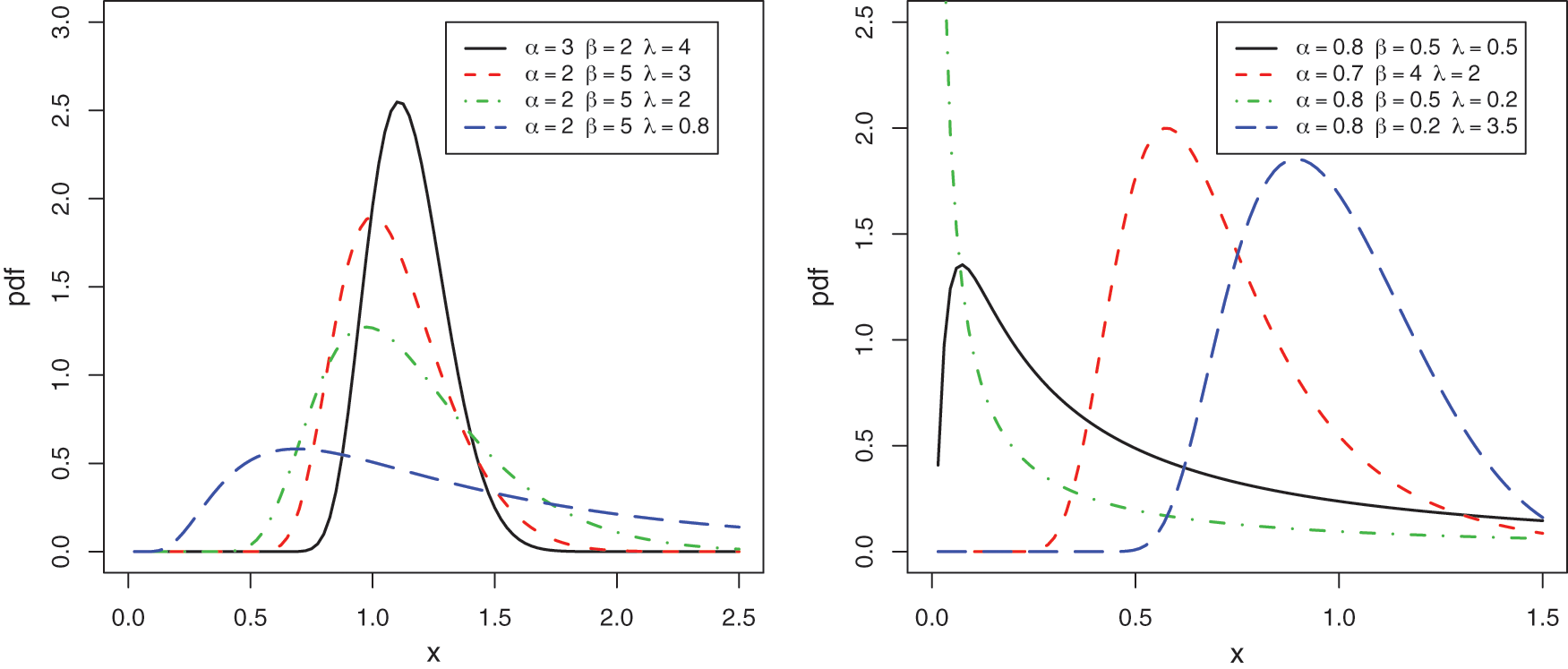
Figure 1: Some curves of the PDF of the TGFrW distribution

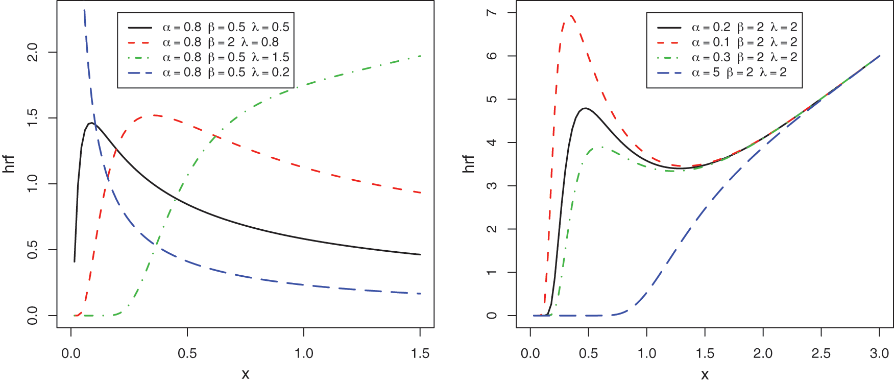
Figure 2: Some curves of the HRF of the TGFrW distribution

In Fig. 1, various degrees of skewness (asymmetry) and kurtosis are observed for , showing decreasing and bell shapes, as well various weights on the right tail mainly. In Fig. 2, we see that possesses reversed J, bathtub decreasing and increasing shapes, with possibly several critical points.

Thanks to (5), the QF can be expressed as

Hence, quartiles and random generations numbers from the TGFrW distribution can be easily investigated.

4.2 Some Properties and Numerical Works

The general properties studied for the TGFr-G family in Section 2 can be applied to the TGFrW distribution. A selection of them are presented below. First of all, in order to complete the observations made on Figs. 1 and 2, let us investigate the equivalences and limits of and . When , we have

Also, when , we have

In particular, we note that plays the major role in these convergence, in all cases, and, when , has the same comportment to the HRF of the parental distribution, i.e., when , when , and when .

Also, by the Riemann integral criteria, the equivalence results for ensure that the raw moments of all orders of exist, for all the values of the parameters. In this setting, let us now discuss the rth incomplete moment of X, rth raw moment of X with related measures, and the Tsallis entropy.

As usual, the rth incomplete moment of X can be expressed as its principal integral form. Alternatively, owing to (7) and the equality: , where denotes the lower incomplete gamma function, we have

We can manipulate this expansion to derive approximations of the measures and functions presented in Subsection 3.5. Also, by applying , we get the rth raw moment of X, i.e.,

where . As numerical works, Tabs. 5 and 6 collected the numerical values of some measures of the TGFrW distribution derived to the raw moments.

Table 5: Values of some measures of the TGFrW distribution for several values of and at

Table 6: Values of some measures of the TGFrW distribution for several values of and at and

Among others, Tabs. 5 and 6 show how the values of some moments measures of can vary according to the values of the parameters. Here, a great variation of the values on the mean and kurtosis are mainly observed.

As described in Subsection 3.6, the Tsallis entropy of the TGFrW distribution is initially defined by an integral expression. A tractable series expansion can be deduced from (9). Indeed, since provided that , we have

Possible values for the Tsallis entropy are shown in Tab. 7.

Table 7: Values of the Tsallis-entropy of the TGFrW distribution for several values of the parameters

Tab. 7 reveals that the amount of randomness of the TGFrW distribution measured by the Tsallis entropy is versatile. Indeed, it can take negative values, as well as small or large positive values. The rest of the study focuses on the statistical usefulness of the TGFrW model in a statistical framework.

4.3 Estimation: Numerical Study

The ML estimates of the parameters of the TGFrW model, the corresponding CIs and the estimate of the Tsallis entropy can be obtained via the approach described in Subsection 3.7. Here, we provide a numerical study on these statistical objects through the simple random sampling scheme. This scheme is based on the QF defined by (10). A performance study of the estimates is conducted relatively to the mean square errors (MSEs), (average) LBs and UBs of the corresponding 90% and 95% CIs, as well as the corresponding average lengths (ALs), i.e., . The software Mathematica 9 is used in this regard. The following steps are followed.

Step 1: A random sample of values of size n = 100, 200, 300, 1000 and 3000 is generated from the TGFrW distribution.

Step 2: We consider the following sets of parameters: set1: (, , ), set2: (, , ), set3: (, , ) and set4: (, , ).

Step 3: For each of the above sets and each sample of size n, the ML estimates are computed.

Step 4: We repeat the previous steps N times, dealing with different samples, where N = 5000. Then, the MSEs of the estimates are computed.

Step 5: Also, the LBs, UBs and ALs of the 90% and 95% CIs are calculated.

Step 6: Numerical outcomes are given in Tabs. 8–11.

Table 8: Values of ML estimates and IC measures related to the TGFrW model for set1: (, , )

Table 9: Values of ML estimates and IC measures related to the TGFrW model for set2: (, , )

Table 10: Values of ML estimates and IC measures related to the TGFrW model for set3: (, , )

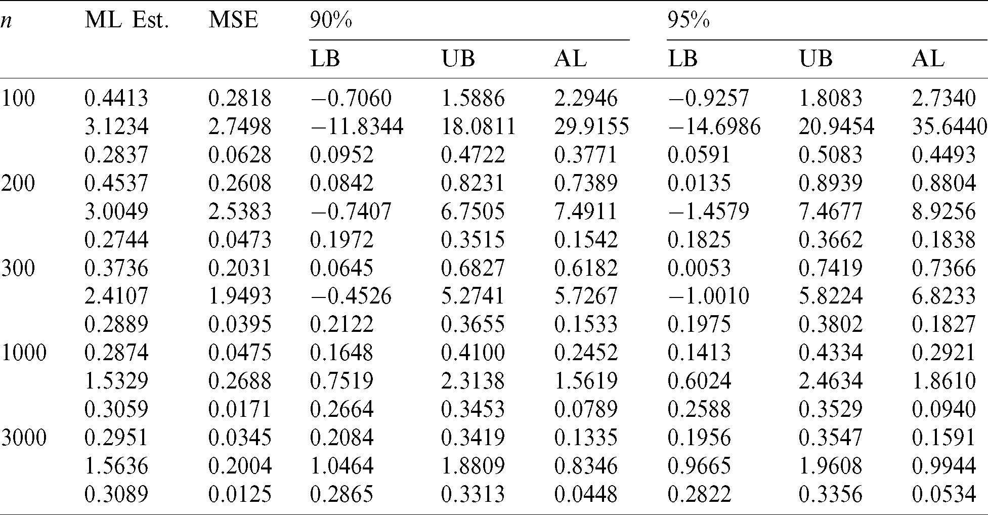
Table 11: Values of ML estimates and IC measures related to the TGFrW model for set4: (, , )

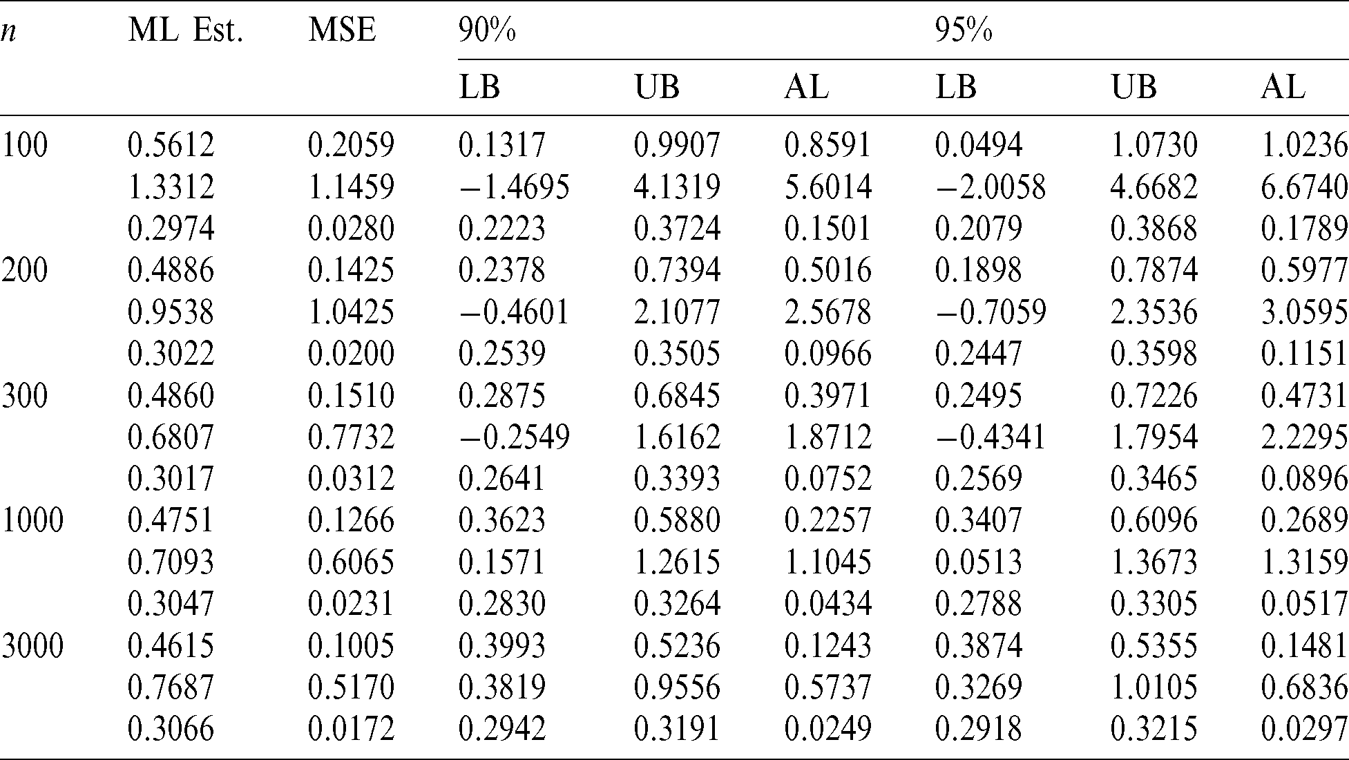
For all the considered sets of parameters, the values in Tabs. 8–11, indicate that the ML estimates stabilize to the right values as n increases. Also, the MSEs and ALs decrease and tend to 0 as n becomes large as expected.

Now, we check the numerical performance of the estimate of the Tsallis entropy of the TGFrW model as described in Subsection 3.7. In this regard, Tabs. 12–15 list the values of this estimate under the simulation scenario described above. We adopt the criteria of the relative bias (RB), defined as .

Table 12: Values of the Tsallis entropy estimates related to the TGFrW model for set 1: (, , )

Table 13: Values of the Tsallis entropy estimates related to the TGFrW model for set 2: (, , )

Table 14: Values of the Tsallis entropy estimates related to the TGFrW model for set 3: (, , )

Table 15: Values of the Tsallis entropy estimates related to the TGFrW model for set 4: (, , )

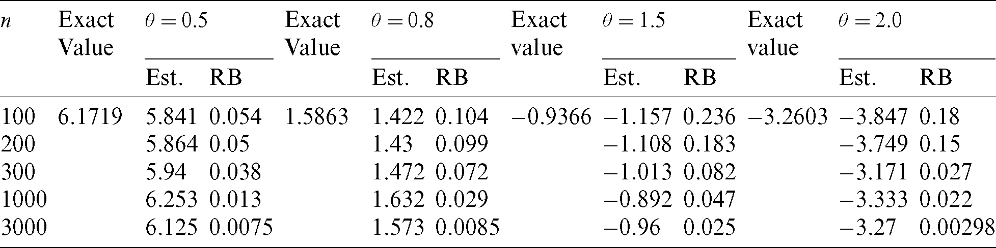
For all the considered sets of parameters, the values in Tabs. 8–11, indicate that the estimates of the Tsallis entropy stabilize to the exact values as n increases. Also, the RBs decrease and tend to 0 as n becomes large, which is a consistent observation with the expected theoretical convergence.

4.4 Data Analysis

Here, we show that the TGFrW model is ideal to fit practical data of various kinds, with better results in comparison to solid extended Weibull models. More specifically, the two following data sets are considered.

The first data set, called datasetI, contains 100 observations on minutes waiting time before a client receives the desired service in a bank. It is: datasetI = {0.8, 0.8, 1.3, 1.5, 1.8, 1.9, 1.9, 2.1, 2.6, 2.7, 2.9, 3.1, 3.2, 3.3, 3.5, 3.6, 4, 4.1, 4.2, 4.2, 4.3, 4.3, 4.4, 4.4, 4.6, 4.7, 4.7, 4.8, 4.9, 4.9, 5.0, 5.3, 5.5, 5.7, 5.7, 6.1, 6.2, 6.2, 6.2, 6.3, 6.7, 6.9, 7.1, 7.1, 7.1, 7.1, 7.4, 7.6, 7.7, 8, 8.2, 8.6, 8.6, 8.6, 8.8, 8.8, 8.9, 8.9, 9.5, 9.6, 9.7, 9.8, 10.7, 10.9, 11.0, 11.0, 11.1, 11.2, 11.2, 11.5, 11.9, 12.4, 12.5, 2.9, 13.0, 13.1, 13.3, 13.6, 13.7, 13.9, 14.1, 15.4, 15.4, 17.3, 17.3, 18.1, 18.2, 18.4, 18.9, 19.0, 19.9, 20.6, 21.3, 21.4, 21.9, 23, 27, 31.6, 33.1, 38.5}. The reference for this data is [30].

The second data set, called datasetII, represents 30 successive values of precipitation (in inches), in one month, in Minneapolis. It is: datasetII = {0.77, 1.74, 0.81, 1.20, 1.95, 1.20, 0.47, 1.43, 3.37, 2.20, 3.00, 3.09, 1.51, 2.10, 0.52, 1.62, 1.31, 0.32, 0.59, 0.81, 2.81, 1.87, 1.18, 1.35, 4.75, 2.48, 0.96, 1.89, 0.90, 2.05}. The reference for this data is [31].

The following competitors are taken into account: truncated Fréchet-Weibull (TFrW) model proposed by [6], odd log-logistic Weibull (OLLW) model introduced by [32], beta Weibull (BW) model by [33], exponentiated Weibull (EW) model introduced by [34], and gamma-exponentiated exponential (GE) model studied by [35].

For all the models, the estimation of the parameters are performed via the ML method. We refer to Subsection 3.7 concerning the ML estimates of the TGFrW model. As standard criteria of comparison, the following measures are taken into account: , AIC, BIC, W, A, KS and p-value (KS), corresponding to the minus estimated log-likelihood function at the data, Akaike information criterion, Bayesian information criterion, Anderson-Darling statistic, Cramer–von Mises statistic, Kolmogorov–Smirnov statistic and the p-value of the Kolmogorov–Smirnov test, respectively. The corresponding mathematical formulas are described below.

where n is the number of observations, p is the number of parameters of the considered model, are the ordered observations, , where denotes the estimated CDF of the model involving the ML estimates for the parameters and Fn(x) denotes the random empirical CDF. The details on these statistical measures can be found in [36,37].

It is admitted that the smaller the values of AIC, BIC, W, A and KS and the greater the values of p-value (KS), the better the model is to fit to the considered data. The software R is used for all the calculations.

For the considered models, the ML estimates with their related standard errors (SEs) are reported in Tabs. 16 and 17 for datasetI and datasetII, respectively.

Table 16: Values of the ML estimates and SEs for datasetI

Table 17: Values of the ML estimates and SEs for datasetII

In particular, for datasetI, the parameters , and of the TGFrW model are estimated by , and , respectively, and for datasetII, they are estimated by , and , respectively. We remark that the novel parameter is estimated far from 1, making a strong difference between the estimated TGFrW model and the former estimated TFrW model.

From Tabs. 18 and 19, it is clear that the TGFrW model is the best of all, with respect to the considered criteria. In particular, it has p-values (KS) closed to 1. As an important remark, the TGFrW model surpasses the former TFrW model, justifying the importance of the generalization.

Table 18: Values of the considered criteria for datasetI

Table 19: Values of the considered criteria for datasetII

Several kinds of fits of the TGFrW model are shown in Figs. 3 and 4 for datasetI and datasetII, respectively. Specifically, the estimated PDFs of the TGFrW distribution are plotted over the corresponding histograms and the estimated CDFs are plotted over the empirical CDFs. The empirical probabilities versus estimated probabilities (P-P) plots and the empirical quantiles versus estimated quantiles (Q-Q) plots are also shown. In all the cases, a near perfect fit is observed, validating the remarkable performance of the TGFrW model.

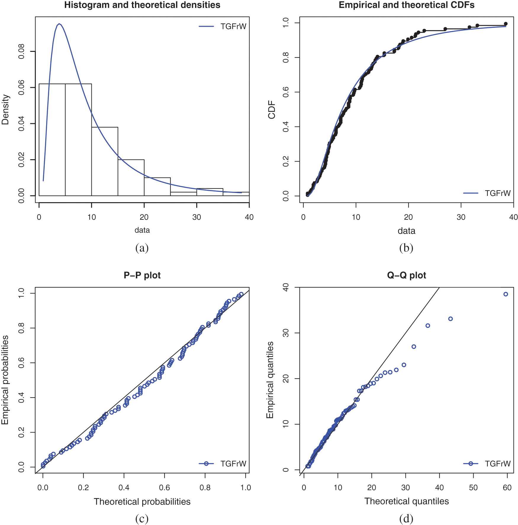
Figure 3: Various fits of the TGFrW model for datasetI: (a) Estimated PDF, (b) estimated CDF, (c) P-P plot and (d) Q-Q plot

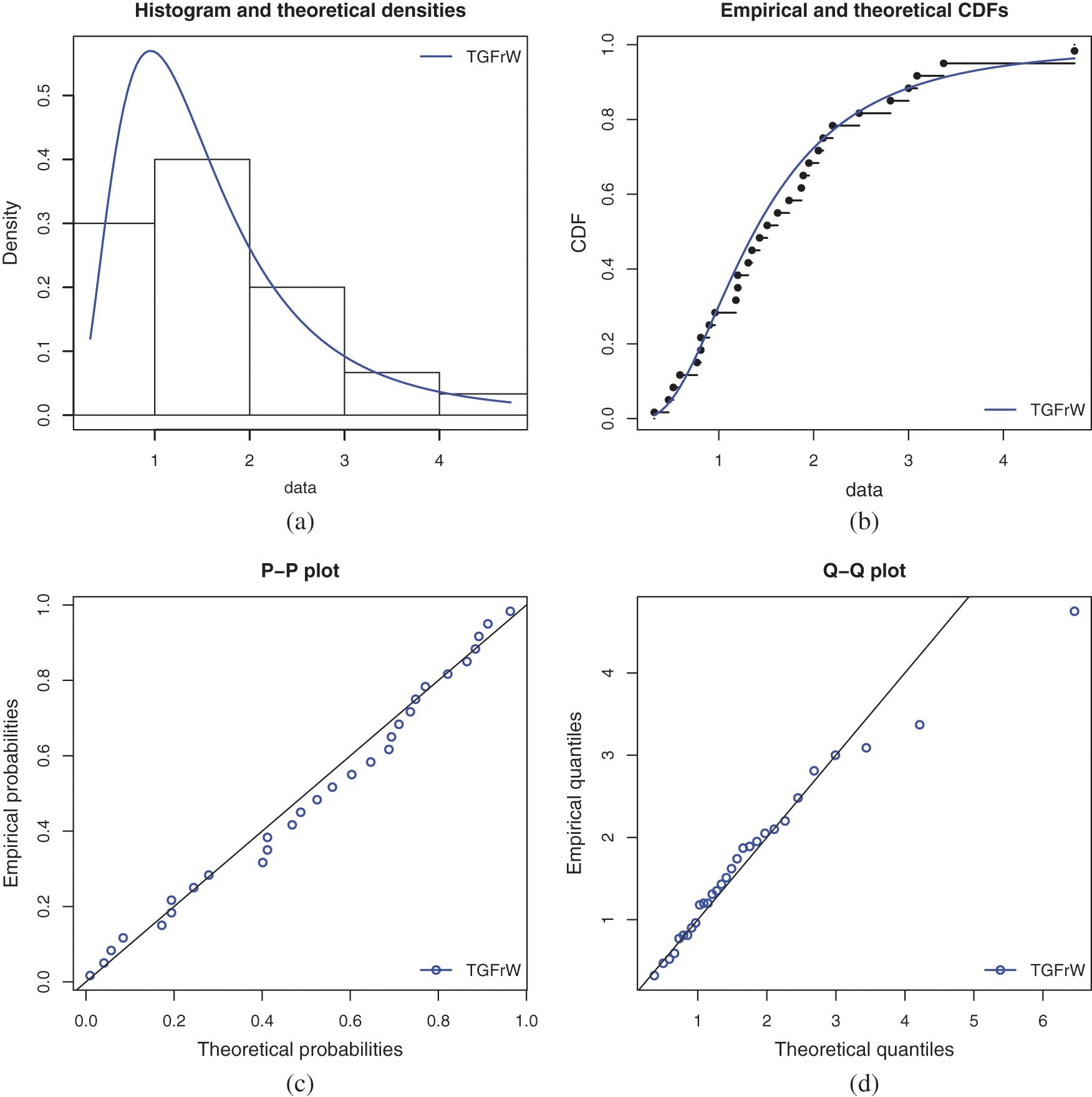
Figure 4: Various fits of the TGFrW model for datasetII: (a) estimated PDF, (b) estimated CDF, (c) P-P plot and (d) Q-Q plot

5  Conclusion

We have motivated the use of the truncated generalized Fréchet distribution to define a new generalized family of continuous distributions, called the truncated generalized Fréchet generated (TGFr-G) family. Diverse mathematical and practical investigations show the full potential of the new family, supported by detailed graphical and numerical evidences. A focus is put on the truncated generalized Fréchet Weibull (TGFrW) distribution, with a complete statistical treatment of the related model. Comparative fitting are performed through the use of two practical data sets, with favorable results to the new model in comparison to other popular extended Weibull models. In particular, under a comparable setting, the new model surpasses the former truncated Fréchet model. As perspectives of future work, other special models of the TGFr-G family may be the subjects of further investigation, specially those with support on . Also, the bivariate extensions of the TGFr-G family can be explored more, with applications in the fields of regression and clustering, for instance. Also, applications in physics remain an interesting challenge, exploring the possible randomness of various networks [38] and various differential equations [39].

Acknowledgement: We thank the reviewers for their thorough comments and remarks which contributed to improve the quality of the paper. This work was funded by the Deanship of Scientific Research (DSR), King AbdulAziz University, Jeddah, under Grant No. (G:531-305-1441). The authors gratefully acknowledge the DSR technical and financial support. The authors, therefore, acknowledge with thanks to DSR technical and financial support.

Funding Statement: This work was funded by the Deanship of Scientific Research (DSR), King AbdulAziz University, Jeddah, under Grant No. G:531-305-1441. The authors gratefully acknowledge the DSR technical and financial support.

Conflicts of Interest: Authors must declare all conflict of interests.

References

 1.  Tahir, M. H., Cordeiro, G. M. (2016). Compounding of distributions: A survey and new generalized classes. Journal of Statistical Distributions and Applications, 3(1), 37. DOI 10.1186/s40488-016-0052-1. [Google Scholar] [CrossRef]

 2.  Brito, C., Rêgo, L., Oliveira, W., Gomes-Silva, F. (2019). Method for generating distributions and classes of probability distributions: The univariate case. Hacettepe Journal of Mathematics and Statistics, 48(3), 897–930. [Google Scholar]

 3.  Ahmad, Z., Hamedani, G. G., Butt, N. S. (2019). Recent developments in distribution theory: A brief survey and some new generalized classes of distributions. Pakistan Journal of Statistics and Operation Research, 15(1), 87–110. DOI 10.18187/pjsor.v15i1.2803. [Google Scholar] [CrossRef]

 4.  Mahdavi, A., Silva, G. (2016). A method to expand family of continuous distributions based on truncated. Journal of Statistical Research Iran, 13, 231–247. [Google Scholar]

 5.  Barreto-Souza, W., Simas, A. B. (2013). The exp-G family of probability distributions. Brazilian Journal of Probability and Statistics, 27(1), 84–109. DOI 10.1214/11-BJPS157. [Google Scholar] [CrossRef]

 6.  Abid, A., Abdulrazak, R. (2017). [0,1] truncated Fréchet-G generator of distributions. Applied Mathematics, 7, 51–66. [Google Scholar]

 7.  Bantan, R., Jamal, F., Chesneau, C., Elgarhy, M. (2019). Truncated inverted Kumaraswamy generated family of distributions with applications. Entropy, 21(1089), 1–22. [Google Scholar]

 8.  Najarzadegan, H., Alamatsaz, M. H., Hayati, S. (2017). Truncated Weibull-G more flexible and more reliable than beta-G distribution. International Journal of Statistics and Probability, 6(5), 1–17. DOI 10.5539/ijsp.v6n5p1. [Google Scholar] [CrossRef]

 9.  Aldahlan, M., Jamal, F., Chesneau, C., Elgarhy, M., Elbatal, I. (2019). The truncated Cauchy power family of distributions with inference and applications. Entropy, 22(346), 1–24. DOI 10.3390/e22010001. [Google Scholar] [CrossRef]

10. Jamal, F., Bakouch, H., Nasir, M. (2020). A truncated general-G class of distributions with application to truncated burr-g family. (in press). [Google Scholar]

11. Aldahlan, M. (2019). Type II truncated Fréchet generated family of distributions. International Journal of Applied Mathematics, 7, 221–228. [Google Scholar]

12. Akbarinasab, M., Arabpour, A., Mahdavi, A. (2019). Truncated log-logistic family of distributions. Journal of Biostatistics and Epidemiology, 5(2), 137–147. [Google Scholar]

13. Alzaatreh, A., Aljarrah, M. A., Smithson, M., Shahbaz, S. H. Shahbaz, M. Q. et al. (2020). Truncated family of distributions with applications to time and cost to start a business. Methodology and Computing in Applied Probability, 42(6), 547. DOI 10.1007/s11009-020-09801-1. [Google Scholar] [CrossRef]

14. Hassan, A., Sabry, M., Elsehetry, A. (2020). A new family of upper-truncated distributions: Properties and estimation. Thailand Statistician, 18(2), 196–214. [Google Scholar]

15. Nadarajah, S., Kotz, S. (2003). The exponentiated Fréchet distribution. Interstat Electronic Journal, 1–7. [Google Scholar]

16. Okorie, I. E., Akpanta, A. C., Ohakwe, J. (2016). The exponentiated Gumbel type-2 distribution: Properties and application. International Journal of Mathematics and Mathematical Sciences, 2016(2), 1–10. DOI 10.1155/2016/5898356. [Google Scholar] [CrossRef]

17. Gupta, R., Kundu, D. (2001). Exponentiated exponential family: An alternative to Gamma and Weibull distributions. Biometrical Journal, 43, 117–130. [Google Scholar]

18. Mansour, M., Aryal, G., Afify, A., Ahmad, M. (2018). The Kumaraswamy exponentiated Fréchet distribution. Pakistan Journal of Statistics, 34(3), 177–193. [Google Scholar]

19. Surles, J. G., Padgett, W. J. (2001). Inference for reliability and stress-strength for a scaled Burr-type X distribution. Lifetime Data Analysis, 7(2), 187–200. DOI 10.1023/A:1011352923990. [Google Scholar] [CrossRef]

20. Kotz, S., Lumelskii, Y., Pensky, M. (2003). The stress-strength model and its generalization: Theory and applications. Singapore: World Scientific. [Google Scholar]

21. Cordeiro, G., Silva, R., Nascimento, A. (2020). Recent advances in lifetime and reliability models. Sharjah, UAE: Bentham Books. [Google Scholar]

22. Amigo, J., Balogh, S., Hernandez, S. (2018). A brief review of generalized entropies. Entropy, 20(11), 813. DOI 10.3390/e20110813. [Google Scholar] [CrossRef]

23. Rényi, A. (1961). On measures of entropy and information. Proceedings of the Fourth Berkeley Symposium on Mathematical Statistics and Probability, vol. 1, pp. 547–561, Univ. of California Press. [Google Scholar]

24. Havrda, J., Charvát, F. (1967). Quantification method of classification processes, concept of structural -entropy. Kybernetika, 3(1), 30–35. [Google Scholar]

25. Arimoto, S. (1971). Information-theoretical considerations on estimation problems. Information and Control, 19(3), 181–194. DOI 10.1016/S0019-9958(71)90065-9. [Google Scholar] [CrossRef]

26. Awad, A., Alawneh, A. (1987). Application of entropy to a life-time model. IMA Journal of Mathematical Control and Information, 4(2), 143–148. DOI 10.1093/imamci/4.2.143. [Google Scholar] [CrossRef]

27. Tsallis, C. (1988). Possible generalization of Boltzmann-Gibbs statistics. Journal of Statistical Physics, 52(1–2), 479–487. DOI 10.1007/BF01016429. [Google Scholar] [CrossRef]

28. Casella, G., Berger, R. (1990). Statistical inference. Bel Air, CA, USA: Brooks/Cole Publishing Company. [Google Scholar]

29. Nelsen, R. (2006). An introduction to copulas. 2nd edition, New York: Springer-Verlag. [Google Scholar]

30. Ghitany, M. E., Atieh, B., Nadarajah, S. (2008). Lindley distribution and its application. Mathematics and Computers in Simulation, 78(4), 493–506. DOI 10.1016/j.matcom.2007.06.007. [Google Scholar] [CrossRef]

31. Hinkley, D. (1977). On quick choice of power transformations. Journal of the Royal Statistical Society, Series C, Applied Statistics, 26, 67–69. [Google Scholar]

32. Cordeiro, G. M., Alizadeh, M., Ozel, G., Hosseini, B., Ortega, E. M. M. et al. (2016). The generalized odd log-logistic family of distributions: Properties, regression models and applications. Journal of Statistical Computation and Simulation, 87(5), 908–932. DOI 10.1080/00949655.2016.1238088. [Google Scholar] [CrossRef]

33. Lee, C., Famoye, F., Olumolade, O. (2007). Beta-weibull distribution: Some properties and applications to censored data. Journal of Modern Applied Statistical Methods, 6(1), 173–186. DOI 10.22237/jmasm/1177992960. [Google Scholar] [CrossRef]

34. Pal, M., Ali, M., Woo, J. (2006). Exponentiated Weibull distribution. Statistica, 66(2), 139–147. [Google Scholar]

35. Ristić, M. M., Balakrishnan, N. (2012). The gamma-exponentiated exponential distribution. Journal of Statistical Computation and Simulation, 82(8), 1191–1206. DOI 10.1080/00949655.2011.574633. [Google Scholar] [CrossRef]

36. Chen, G., Balakrishnan, N. (2018). A general purpose approximate goodness-of-fit test. Journal of Quality Technology, 27(2), 154–161. DOI 10.1080/00224065.1995.11979578. [Google Scholar] [CrossRef]

37. Massey, F. J. Jr. (1951). The Kolmogorov-Smirnov test for goodness of fit. Journal of the American Statistical Association, 46(253), 68–78. DOI 10.1080/01621459.1951.10500769. [Google Scholar] [CrossRef]

38. Liu, J. B., Zhao, J., Cai, Z. Q. (2020). On the generalized adjacency, Laplacian and signless Laplacian spectra of the weighted edge corona networks. Physica A: Statistical Mechanics and Its Applications, 540, 123073. DOI 10.1016/j.physa.2019.123073. [Google Scholar] [CrossRef]

39. Akgül, A. (2018). A novel method for a fractional derivative with non-local and non-singular kernel. Chaos, Solitons & Fractals, 114, 478–482. DOI 10.1016/j.chaos.2018.07.032. [Google Scholar] [CrossRef]

This work is licensed under a Creative Commons Attribution 4.0 International License, which permits unrestricted use, distribution, and reproduction in any medium, provided the original work is properly cited.