| Computer Modeling in Engineering & Sciences |
DOI: 10.32604/cmes.2021.014244
ARTICLE
An Improved Higher-Order Time Integration Algorithm for Structural Dynamics
1Institute of Solid Mechanics, Beihang University, Beijing, 100083, China
2Shen Yuan Honors College, Beihang University, Beijing, 100083, China
*Corresponding Author: Yufeng Xing. Email: xingyf@buaa.edu.cn
Received: 13 September 2020; Accepted: 14 October 2020
Abstract: Based on the weighted residual method, a single-step time integration algorithm with higher-order accuracy and unconditional stability has been proposed, which is superior to the second-order accurate algorithms in tracking long-term dynamics. For improving such a higher-order accurate algorithm, this paper proposes a two sub-step higher-order algorithm with unconditional stability and controllable dissipation. In the proposed algorithm, a time step interval [tk, tk + h] where h stands for the size of a time step is divided into two sub-steps [tk,  ] and [
 , tk + h]. A non-dissipative fourth-order algorithm is used in the first sub-step to ensure low-frequency accuracy and a dissipative third-order algorithm is employed in the second sub-step to filter out the contribution of high-frequency modes. Besides, two approaches are used to design the algorithm parameter
  . The first approach determines
  by maximizing low-frequency accuracy and the other determines
  for quickly damping out high-frequency modes. The present algorithm uses
  to exactly control the degree of numerical dissipation, and it is third-order accurate when
  and fourth-order accurate when
  . Furthermore, the proposed algorithm is self-starting and easy to implement. Some illustrative linear and nonlinear examples are solved to check the performances of the proposed two sub-step higher-order algorithm.
Keywords: Time integration algorithm; two-sub-step; higher-order accuracy; controllable dissipation; unconditional stability
Time integration algorithms are a powerful tool for solving structural dynamics. The accuracy, efficiency, stability, and numerical dissipation have always been important factors when designing a new algorithm or improving an existing algorithm. Based on different design ideas, researchers have developed many types of time integration algorithms, such as the  -algorithms, the composite algorithms, the conserving energy algorithms, and the higher-order algorithms.
To introduce algorithmic dissipation as well as maintain second-order accuracy, the  -algorithms [1–3] like the HHT-
 algorithm, the three-parameter algorithm were developed. By introducing additional parameters in motion equations, the
  -algorithms can achieve this goal. Algorithmic dissipation is beneficial to filtering out high-frequency modes and improving stability of time integration algorithms in solving nonlinear systems. However, such
  -algorithms with algorithmic dissipation cause more amplitude and phase errors in the low-frequency region compared to non-dissipative algorithms [4], such as the trapezoidal rule and the central difference algorithm.
To improve low-frequency accuracy of the  -algorithms, multi-sub-step composite algorithms were developed. The composite concepts first appeared in Bank et al.’s work [5], and they developed a two-sub-step algorithm where the trapezoidal rule and the backward difference formula were combined in a time step. Afterwards, this work was extended to the structural dynamics systems by Bathe in 2005 [6]. In Bathe’s work, the trapezoidal rule was used in the first-sub-step to maintain low-frequency accuracy as much as possible and the second-sub-step adopted backward difference formula to filter out high-frequency mode contribution. Motivated by these works, some composite algorithms with better numerical properties were proposed in the last two decades, such as the two-sub-step algorithms [7–9], the three-sub-step algorithms [10–15] and the four-sub-step algorithms [13,14].
To solve nonlinear systems, conserving energy algorithms were developed. Different from  -algorithms and composite algorithms, the construction of conserving energy algorithms is based on the energy principle [16]. Most conserving energy algorithms [17–22] can handle the geometric nonlinearity problems and one [23] can deal with the systems including geometric nonlinearity and damping nonlinearity.
To satisfy the pursuit for high accurate solutions, higher-order algorithms [24–32] were developed. The series algorithms, such as the Taylor series algorithm and the Lie series algorithm, are classical higher-order algorithms, which cannot be unconditionally stable when the accuracy order is more than two [25]. For keeping higher-order accuracy and improving stability, the multi-stages implicit Runge–Kutta algorithm [26], the weighted-residual method-based algorithms [27,28] and the differential quadrature algorithms [29–31] were proposed. Compared to second-order accurate algorithms, higher-order algorithms can use larger time step size and have advantages in long-term tracking. In 2017, the higher-order algorithms based on the weighted residual method proposed by Kim et al. [28] have the nth-order ( ) accuracy and unconditional stability with controllable algorithmic dissipation, but the algorithms’ stability for nonlinear problems needs to be improved.
As can be seen from above review that (1) there are no multi-sub-step time integration algorithms that have higher-order accuracy, unconditional stability and controllable dissipation; (2) the designs of existing time integration algorithms mainly take accuracy, stability and dissipation into account rather than the properties of dynamic systems.
In this context, this work is to construct a two sub-step higher-order algorithm based on the Kim’s work [28]. In the proposed algorithm, a time step [tk, tk + h] is divided into two sub-steps, [tk,  ] and [
 , tk + h]. Both sub-steps employ the Kim scheme with two collocation points. To obtain better performance, two approaches are provided for determining the parameter
  . The first one is to maximize low-frequency accuracy, in which the value of
  is determined by
  where PE denotes percentage period elongation [33]. The second is for quickly eliminating high-frequency contribution, and the algorithm with such
  can perform better in the rigid-flexible coupling and wave propagation systems.
The rest of the paper is organized as follows. Section 2 presents the formulations of the proposed two sub-step algorithm and the determination method of the parameter  . The numerical properties of the proposed algorithm are discussed in Section 3. Numerical comparisons are provided in Section 4. Finally, the conclusions are drawn in Section 5.
2 The Two Sub-Step Higher-Order Algorithm
This section gives the formulations of the proposed algorithm, in which a time step [tk, tk + h] is divided into two sub-steps as [tk,  ] and [
 , tk + h] where h stands for the time step size.
2.1 The First Sub-Step Formulations
By using the Lagrange interpolation functions  (i = 0, 1, 2), the displacement
  , velocity
  , and acceleration
  in the first sub-step are expressed as


where  and the Lagrange interpolation functions are

The displacement, velocity, and acceleration vectors shown in Eqs. (1)–(3) are independent of each other, so two residuals are introduced to describe the velocity–displacement relationship and the acceleration–velocity relationship. The two residuals have the forms as


For exact solutions,  and
and  are equal to zero. To achieve accurate approximate solutions, here the residuals
  and
and  are minimized with the following weighted equations as


where 
 is the weighting function. Substituting Eqs. (1)–(3) into Eqs. (7) and (8) leads to the velocity–displacement and the acceleration–velocity relationships in matrix form as


where  (i, j = 1, 2),
  (i = 1, 2), and
  (i = 1, 2) are all the functions of
  and
and  which are

where the superscript ‘1’ represents the first sub-step, and  and
and  can be determined by maximizing the order of accuracy. For this end, consider a single degree-of-freedom system as follows

where  and
and  denote the physical damping ratio and natural frequency respectively. In terms of the Eqs. (9) and (10) and for this simple system (12), one can obtain a recursive formulation for first sub-step as

where  is the transfer matrix. The order of accuracy can be designed with the help of local truncation error
  [33], of which the definition is

where  and
and  , which are the functions of
  and
and  . If
. If  where l > 0, the method is lth-order accurate. Through the Taylor series expansion of displacement at t = tk, the explicit expressions of
  can be obtained as

It follows that the first sub-step method is at least second-order accurate and is fourth-order accurate if  and
and  . Fortunately, the spectral radius
  is equal to 1 when
  and
and  . With the relations between (
 ,
,  ) and (
 ,
,  ,
,  ), one can have

For obtaining the unknown vectors  ,
,  , and
, and  in the first-sub-step, we consider the following equilibrium equations at the time nodes of
  and
and  , which have the forms as

where  ,
,  and
and  are the mass, damping and stiffness matrices;
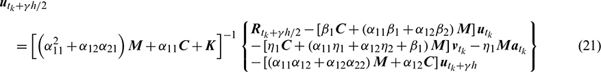
  is the external load vector. Substituting Eqs. (9) and (10) into Eq. (17) yields
  as
as

The above effective stiffness matrix  and the effective external load vector
  have the forms as


where

Then the unknown vectors  can be obtained as
Then, by substituting  and
and  into Eqs. (9) and (10), one can arrive at
  , and
, and  . And
. And  ,
,  , and
, and  are the initial conditions of the second sub-step. It is noteworthy that the weighted residual method is a common way in the construction of time integration algorithms. It can be seen from Eqs. (5)–(7) that in the present algorithm, the inherent relations between displacement, velocity, and acceleration are only satisfied in a weak form, but the equilibrium equations are satisfied strictly at discrete points, as shown in Eq. (17).
2.2 The Second-Sub-Step Formulations
As in the first sub-step,  ,
,  and
and  within
  can also be approximated using the Lagrange interpolation function, as


where

The velocity–displacement and acceleration–velocity relationships have the matrix forms as
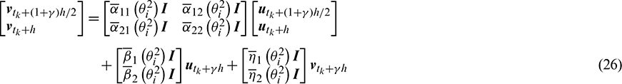

where  ,
,  ,
,  (i, j = 1, 2) are the functions of
  and
and  . For the system (12), one can also obtain a recursive formulation like Eq. (13), as

where  is the transfer matrix. Also, according to local truncation error analysis, we can find a relationship of
  and
and  as
as

which makes the second sub-step method third-order accurate. In terms of the spectral radius of  , the following relation can be achieved as

Then the parameter  is introduced to control the damping of the present algorithm. By using Eqs. (29) and (30), all free parameters in the second sub-step can be explicitly expressed in terms of
  as
as
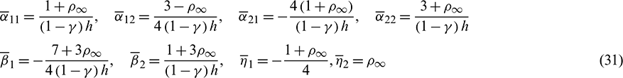
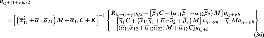
With these parameters, the method for the second sub-step is unconditionally stable. To calculate the results at tk + h, we take the equilibrium equations at  and tk + h into account as

Substituting Eqs. (26) and (27) into Eq. (32) leads to the displacement  as
as

The effective stiffness matrix  and the effective external load vector
  are
are


where

and the displacement  can be obtained by
By inserting  and
and  into Eqs. (26) and (27), we can achieve
  , and
, and  .
.
2.3 Determination of the Parameter 
This sub-section aims to present two approaches for determining the last free parameter  , the ratio of the first sub-step size and the entire step size.
The first approach is to preserve low-frequency mode contribution as much as possible. To reach this end, the value of  is determined by minimizing percentage period error. Since the explicit relation among
  ,
,  and the phase elongation is complex, the optimal
  for some
  are listed in Tab. 1. For clearer showing whether or not these values of
  make the phase error minimum, Figs. 1 and 2 show the percentage amplitude decay and the period elongation vs.
  for
for  , and Figs. 3 and 4 display the results for
  . It can be seen that these values of
  can really minimize period elongations, noting that at the minimum point the amplitude decay is also close to the minimum. To simply obtain the optimal
  for any
  , a fitting algebraic relationship between
  and the optimal
  is provided as

Table 1: The relationships between the optimal  and
and 

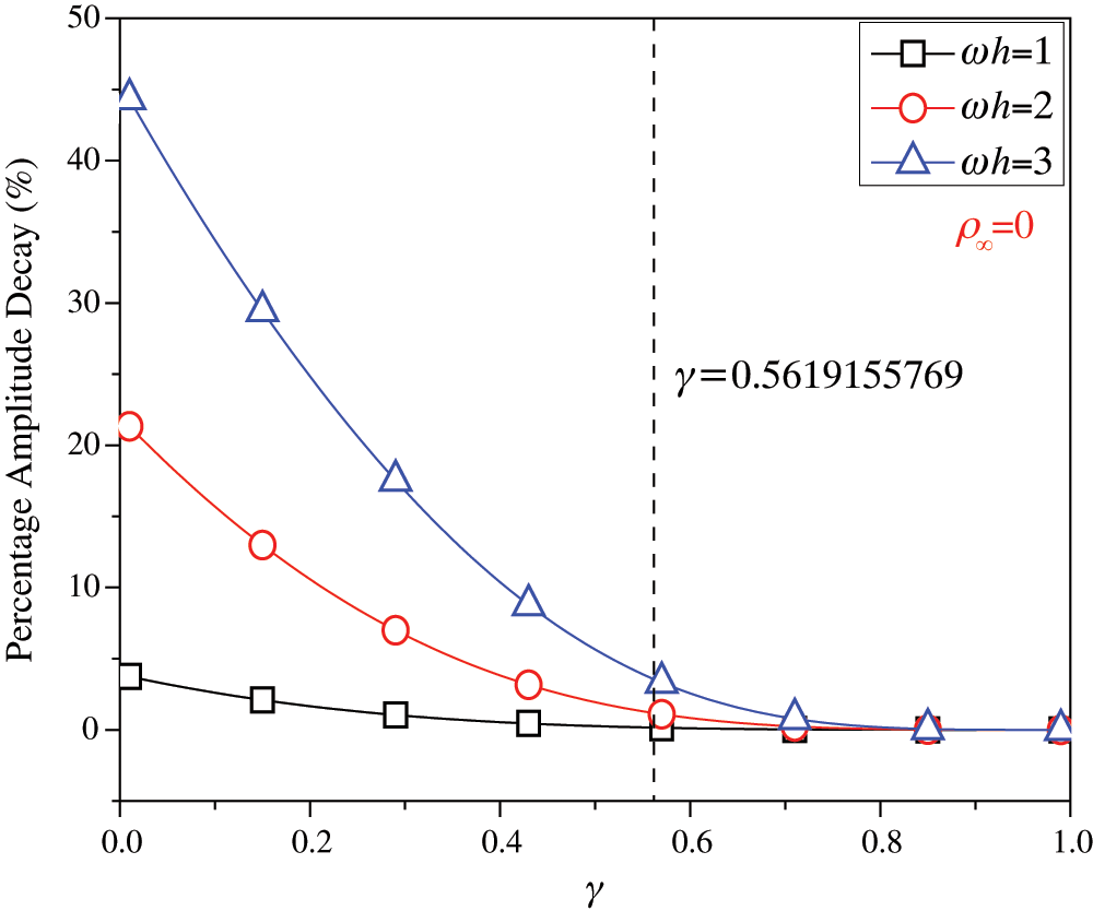
Figure 1: Percentage amplitude decay vs.  (
( ,
,  )
)
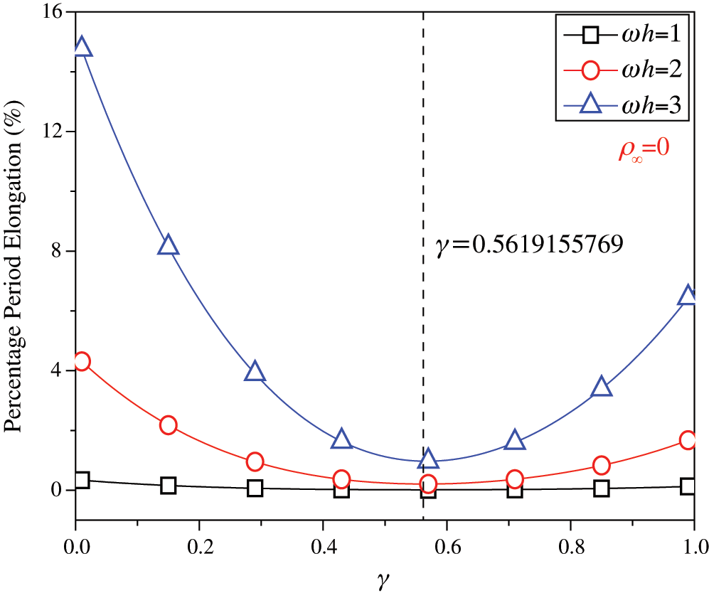
Figure 2: Percentage period elongation vs.  (
( ,
,  )
)
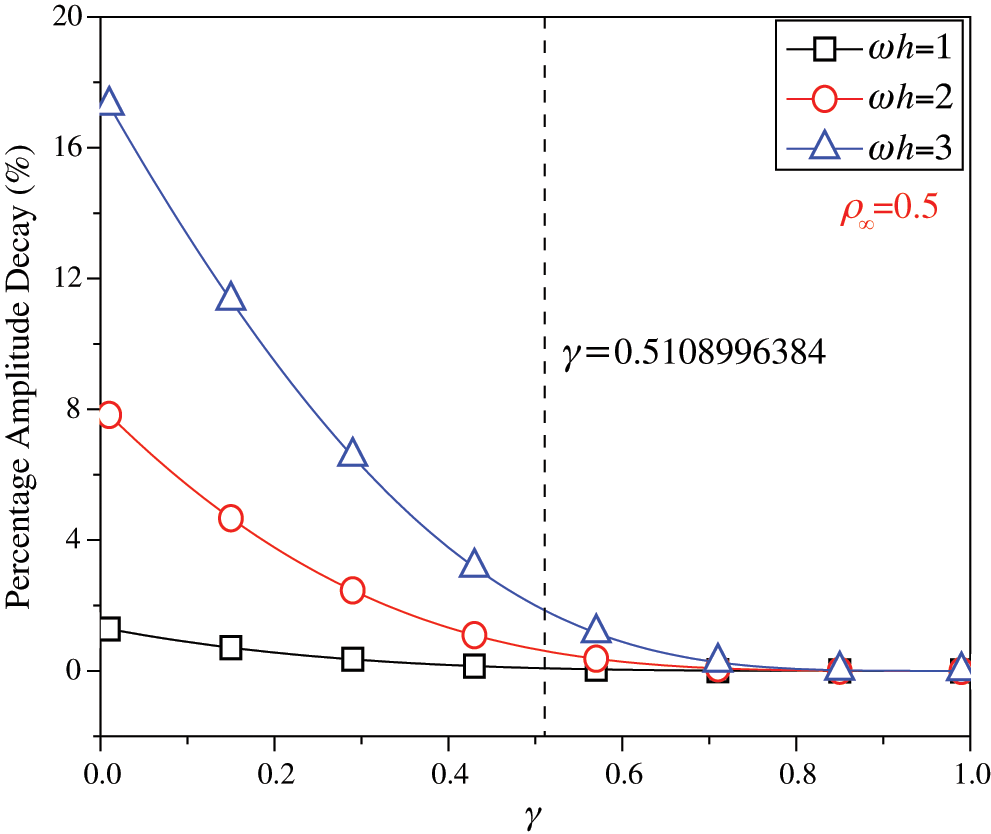
Figure 3: Percentage amplitude decay vs.  (
( ,
,  )
)
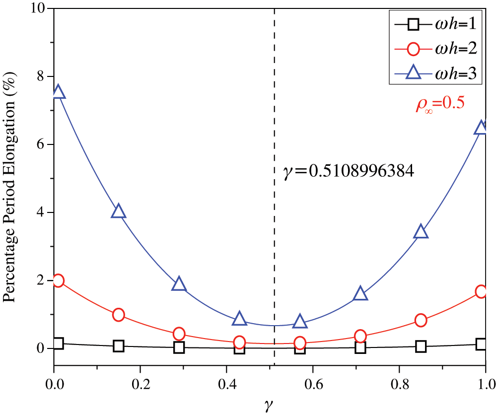
Figure 4: Percentage period elongation vs.  (
( ,
,  )
)
Fig. 5 shows the fitted and true values of  . The proposed algorithm using the
  in Eq. (37), denoted by ‘Present 1’ in this paper, is recommended for most dynamics problems.
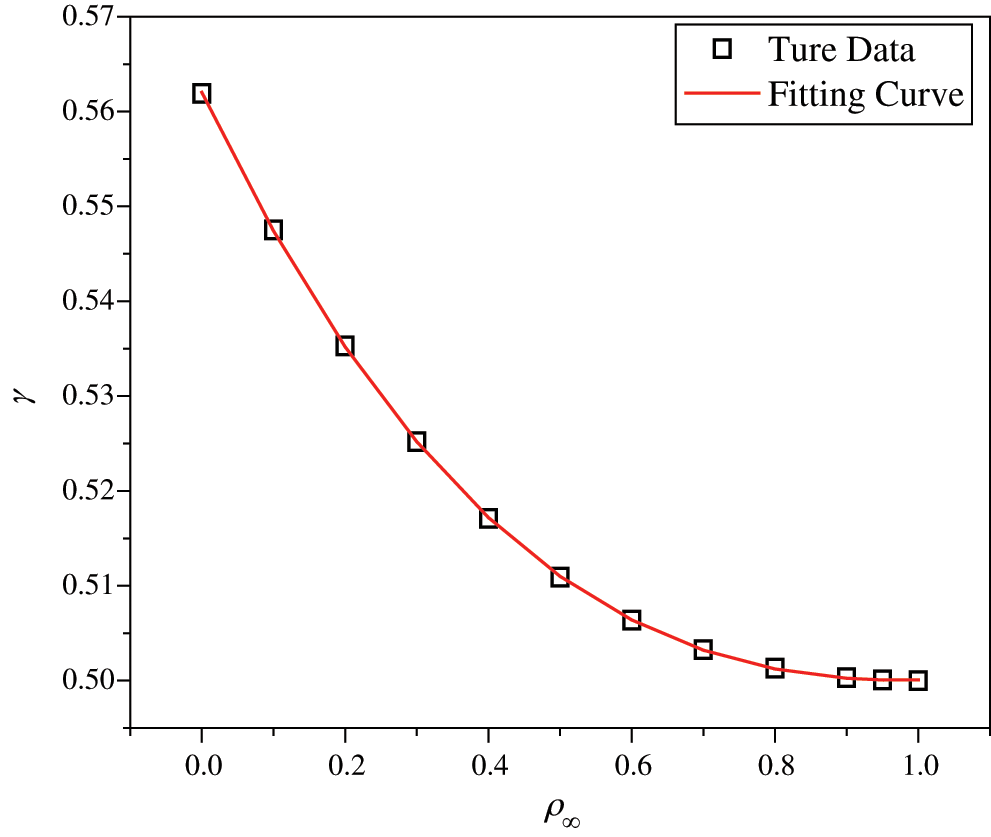
Figure 5: The comparisons between the fitted values and the true values
For rigid-flexible coupling and wave propagation problems, time integration algorithms that can quickly damp out high-frequency effects are expected. To achieve such a capability, the parameter  can be determined by the following second approach.
Fig. 6 shows the variations of the percentage amplitude decay of the proposed algorithm with  and
and  for the case of
  , and the result of
  is provided in Fig. 7. It can be seen that the percentage amplitude decay curves are symmetric about
  for any values of
  . Fig. 8 shows the spectral radius vs.
  for several given
  , indicating that the larger amount of numerical dissipation can be obtained in the low-frequency range with a larger
  .
.

Figure 6: The variations of percentage amplitude decay with  and
and  (
( )
)
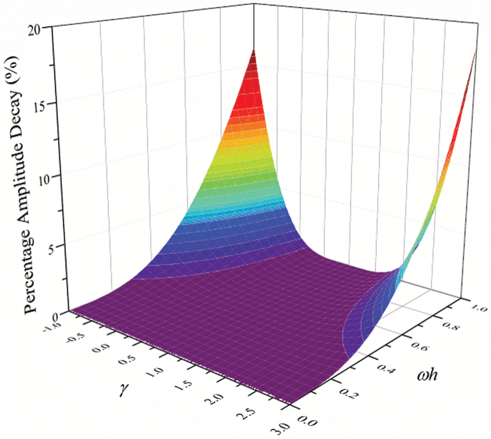
Figure 7: The variations of percentage amplitude decay with  and
and  (
( )
)

Figure 8: Spectral radius vs.  and
and  (
( ): (a)
  ; (b)
; (b) 
As is well known, most time integration algorithms with controllable dissipation possess the biggest amount of dissipation when  . It can be seen from Figs. 6–8 that the amount of dissipation can be improved further by adjusting the values of
  for the proposed algorithm. For ensuring the accuracy of low-frequency response, the value of
  satisfying
  is suggested, refer to Fig. 8. The proposed algorithm using the value of
  determined by this approach is denoted by ‘Present 2’ in the numerical comparisons in Section 4.
After determining  , the construction of the present algorithm is completed, and its flowchart and step-by-step implementing procedure are presented in Fig. 9 and Tab. 2 respectively. Using the Newton iteration method, the proposed algorithm is also applicable to the general nonlinear dynamics as

where  is the nonlinear resilience force.

Figure 9: Flowchart of the proposed algorithm for linear systems
Table 2: Step-by-step implementing procedure of the proposed algorithm for linear systems

This section is to discuss the proposed algorithm’s properties, including efficiency, stability, dissipation, accuracy, and convergence rates. In this work, the present algorithm is compared with the single-step fourth-order Kim method [28], the single-step fourth-order IHOA-4 [32], and the two-sub-step second-order  -Bathe method [7]. The accuracy of different types of algorithms should be compared under the same computational cost. In terms of the number of times the equilibrium equation is used in a time step, the time step sizes of these algorithms should satisfy
 (Present) (indicating that the step size of IHOA-4 is a quarter of the step size of the present method, for example) to ensure that the accuracy comparison is conducted under roughly equal computational costs.
3.1 Stability, Dissipation and Accuracy
In general, a SDOF system like (12) is used to examine the properties of a time integration algorithm for linear systems. The spectral analysis of Present 2 have been presented Section 2.3.2, so this section mainly discusses the numerical properties of the ‘Present 1’. Figs. 10–12 show the spectral radius vs.  and Figs. 13 and 14 show the percentage amplitude decay and period elongation vs.
  (
( ) where
  /n (n stands for the number of times the equilibrium equation is used in a time element), keeping same computational costs. It can be seen from Figs. 10–12 that the present algorithm is unconditionally stable for undamped and damped systems, and its numerical dissipation can be exactly and smoothly controlled by
  . Figs. 13 and 14 illustrate that (1) if
  , Present 1 almost has the same amplitude and phase accuracy as the Kim algorithm; (2) if
  , Present 1 is more accurate than the Kim algorithm. Since the amplitude errors of them are all zero when
  , the relevant results are not plotted in Fig. 13.
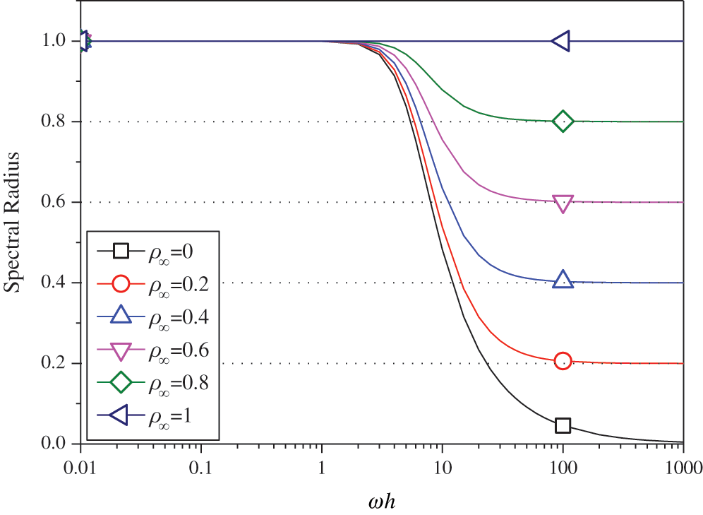
Figure 10: Spectral radius vs.  for Present 1 (
 )
)
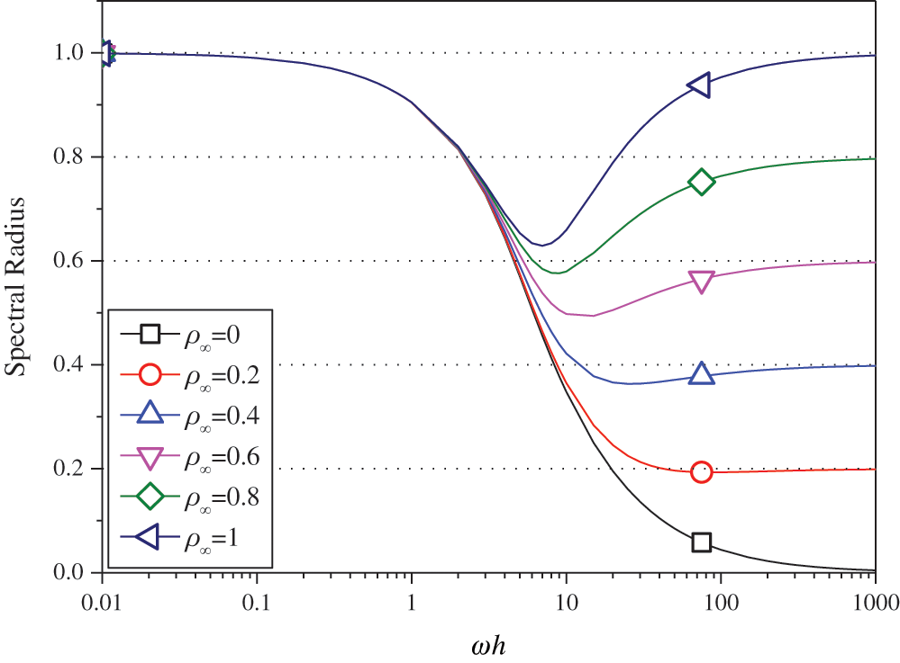
Figure 11: Spectral radius vs.  for Present 1 (
 )
)
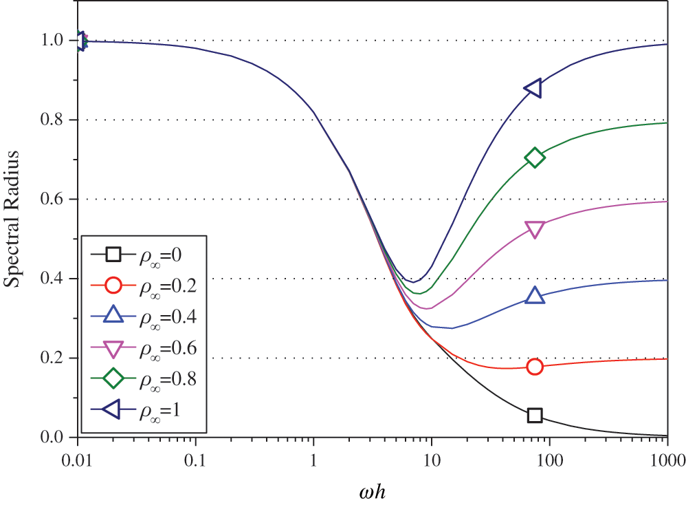
Figure 12: Spectral radius vs.  for Present 1 (
 )
)

Figure 13: Percentage amplitude decay vs.  (
( ) (
) ( )
)

Figure 14: Percentage period elongation vs.  (
( ) (
) ( )
)
The convergence rates of the proposed algorithm are checked in this section. Consider a SDOF system as

where  ,
,  , and the initial displacement and velocity are zero. The decrease rates of absolute errors as the step size decreases are defined as the convergence rates, and displacement, velocity and acceleration may have different convergence rates. The
  -Bathe algorithm [7] is second-order accurate, so its results are plotted here as a reference. The value of the parameter
  has no effect on algorithmic order, refer to Eq. (15), so only the results of Present 1 are shown here.
The undamped case is considered first. Fig. 15 shows the absolute errors of displacement, velocity, and acceleration. It can be seen that the proposed algorithm and the Kim algorithm are both fourth-order accurate when  , and they are both third-order accurate otherwise; the present algorithm is more accurate than the Kim algorithm when 0
  .
.

Figure 15: Convergence rates of the undamped system ( )
)
For the damped case,  is used. It can be seen from Fig. 16 that the proposed algorithm is still fourth-order accurate when
  and third-order accurate when
  .
.

Figure 16: Percentage period elongation vs.  (
( ) (
) ( )
)
To verify the performance of the proposed algorithm, some numerical experiments are conducted here. The proposed algorithm is compared with the Kim algorithm [28], the IHOA-4 [32], and the  -Bathe algorithm [7]. In all simulations, the time step size of the IHOA-4 is provided and the sizes of other algorithms can be determined by the relations of
  (Present).
In this example, consider a linear bi-material bar subjected to a harmonic displacement excitation at the left end [28], as shown in Fig. 17. The motion equation of the bi-material bar is

with the initial and boundary conditions of


Figure 17: A bi-material bar with a harmonic displacement excitation at the left end
The dimensionless mass density, sectional area and length are assumed as  , A = 1 and L = 1 respectively, and the elasticity modulus is
  for
for  and
and  for
for  . Two combinations of E1 and E2 are considered below, and the bar is modelled with two quadratic elements.
4.1.1 The First Case (E1 = 10 and E2 = 1)
This case is used to test the performance of the higher-order accurate algorithms for long-term tracking. The step size  /6 where
  , and the reference solutions are achieved via the mode superposition method. For long-term simulations, numerical dissipation is not expected, so
  is employed in all algorithms. Figs. 18–20 illustrate the results of the middle point of the bar for the time interval [498,500], where one can see that the second-order accurate
  -Bathe algorithm have obvious errors and other fourth-order accurate algorithms’ results agree well with the reference solution.

Figure 18: The displacement of the middle point for the first case

Figure 19: The velocity of the middle point for the first case

Figure 20: The acceleration of the middle point for the first case
4.1.2 The Second Case (E1 = 5000 and E2 = 1)
The second case is designed to show the better performance of numerical dissipation of the proposed algorithm over other higher-order algorithms. The time step size h = 0.005 is used, and  is employed. To better handle the present rigid-flexible coupling problem, the parameter
  of the proposed algorithm is determined by Approach 2. It can be seen from Figs. 21–23 that: (1) the proposed algorithm can eliminate high-frequency effects without introducing excessive errors; (2) the Kim algorithm has obvious numerical oscillations; (3) the IHOA-4 loses stability due to its conditional stability. To make the figure clearer, the acceleration results of the IHOA-4 are omitted in Fig. 22.

Figure 21: The displacement of the middle point for the second case

Figure 22: The velocity of the middle point for the second case

Figure 23: The acceleration of the middle point for the second case
Moreover, the CPU time required by different algorithms in this example are presented in Tab. 3 where one can observe that the computational costs of different algorithms are almost equal when the step sizes satisfy the relation  .
.
Table 3: CPUs of different time integration algorithms in Example 1

Consider a nonlinear pendulum system [17] pinned at the top and free at the bottom, as shown in Fig. 24. The material parameters  N,
N,  kg/m and the length l0 = 3.0443 m are adopted, and the rotation of the pendulum is started by an initial tangential velocity of v0 = 7.72 m/s at the free end. Since the axial stiffness is huge, the motion of the pendulum is like a rigid rotation. A linear truss element is used to model the pendulum, so the system has two DOFs.

Figure 24: Truss model of the rigid pendulum
The step size h = 0.05 s, and  is used. The results of the
  -Bathe algorithm with an extremely small time step size serve as the reference solutions. Figs. 25–27 show the results of the free end in the x direction within [0, 10 s]. It can be seen that the IHOA-4 and the Kim algorithm fail. In fact, this simple problem has also defeated some other famous algorithms, such as the trapezoidal rule. Also, we can find that the
  -Bathe algorithm exhibits phase lag.

Figure 25: Displacement of the free end in the horizontal direction

Figure 26: Velocity of the free end in the horizontal direction
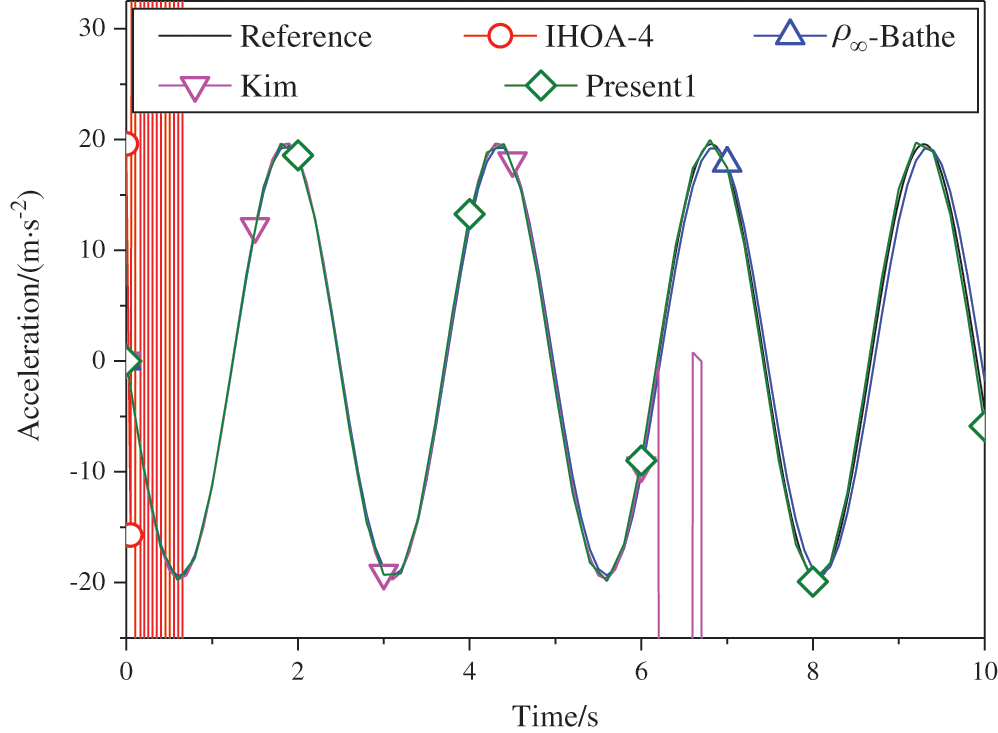
Figure 27: Acceleration of the free end in the horizontal direction
4.3 The Two-Story Shear Building
As shown in Fig. 28, in this example a two-story shear building is considered, which has two degrees of freedom. The lumped masses of the bottom and the top floors are  kg and
  kg, respectively. The nonlinear stiffness for each story is

where  is the initial stiffness and
  represents the story drift. For the bottom story,
  N/m, and the
  N/m is for the top story. Two stores are subjected to the same the external force
  . The coefficients
  and
and  are used for the bottom and top stories respectively. The step size h = 0.0625 s, and
  is used. The reference solution is achieved through the
  -Bathe algorithm with a much smaller step size. Figs. 29–31 provide the results of the top story. One can see that: (1) The non-dissipative IHOA-4 loses stability; (2) The
  -Bathe algorithm and the Kim algorithm have larger errors than the present method.

Figure 28: Two-story shear building

Figure 29: Displacement of the top story

Figure 30: Velocity of the top story

Figure 31: Acceleration of the top story
Based on the single-step Kim algorithm, this work proposed a two sub-step higher-order time integration algorithm with unconditional stability and controllable dissipation. A non-dissipative fourth-order accurate scheme is used in the first sub-step, and a third-order accurate scheme with controllable dissipation is used in the second-sub-step.
As to the determination of the parameter  , the ratio between the first-sub-step size and the entire step size, this work provided two approaches for achieving different goals. One approach maximizes low-frequency accuracy and the other can quickly damp out high-frequency mode effects.
The numerical properties and simulations showed that the present two sub-step algorithm has accuracy, dissipation, and stability advantages over the Kim algorithm and the  -Bathe algorithm.
Funding Statement: This work was supported by the National Natural Science Foundation of China (Grant Numbers 11872090, 11672019 and 11472035).
Conflicts of Interest: The authors declare that they have no conflicts of interest to report regarding the present study.
1. Soares, D. (2015). An explicit time marching technique with solution-adaptive time integration parameters. Computer Modeling in Engineering & Sciences, 107(3), 223–247. [Google Scholar]
2. Shao, H. P., Cai, C. W. (1988). The direct integration three-parameters optimal schemes for structural dynamics. Proceeding of the International Conference: Machine Dynamics and Engineering Applications, C16–C20, Xi’an, China. [Google Scholar]
3. Zhou, X., Tamma, K. K. (2004). Design, analysis, and synthesis of generalized single step single solve and optimal algorithms for structural dynamics. International Journal for Numerical Methods in Engineering, 59(5), 597–668. DOI 10.1002/nme.873. [Google Scholar] [CrossRef]
4. Kwon, S. B., Lee, J. M. (2019). Development of non-dissipative direct time integration method for structural dynamics application. Computer Modeling in Engineering & Sciences, 118(1), 41–89. DOI 10.31614/cmes.2019.03879. [Google Scholar] [CrossRef]
5. Bank, R. E., Coughran, W. M., Fichtner, W., Grosse, E. H., Rose, D. J. et al. (1985). Transient simulations of silicon devices and circuits. IEEE Transactions on Electron Devices, ED-32(10), 436–451. [Google Scholar]
6. Bathe, K. J., Baig, M. M. I. (2005). On a composite implicit time integration procedure for nonlinear dynamics. Computers & Structures, 83(31–32), 2513–2534. DOI 10.1016/j.compstruc.2005.08.001. [Google Scholar] [CrossRef]
7. Noh, G., Bathe, K. J. (2019). The Bathe time integration method with controllable spectral radius: The -Bathe method. Computers & Structures, 212, 299–310. DOI 10.1016/j.compstruc.2018.11.001. [Google Scholar] [CrossRef]
8. Kim, W., Choi, S. Y. (2018). An improved implicit time integration algorithm: The generalized composite time integration algorithm. Computers & Structures, 196, 341–354. DOI 10.1016/j.compstruc.2017.10.002. [Google Scholar] [CrossRef]
9. Kim, W. (2019). A new family of two-stage explicit time integration methods with dissipation control capability for structural dynamics. Engineering Structures, 195, 358–372. DOI 10.1016/j.engstruct.2019.05.095. [Google Scholar] [CrossRef]
10. Ji, Y., Xing, Y. F. (2020). An optimized three-sub-step composite time integration method with controllable numerical dissipation. Computers & Structures, 231, 106210. DOI 10.1016/j.compstruc.2020.106210. [Google Scholar] [CrossRef]
11. Chandra, Y., Zhou, Y., Stanciulescu, I., Eason, T., Spottswood, S. (2015). A robust composite time integration scheme for snap-through problems. Computational Mechanics, 55(5), 1041–1056. DOI 10.1007/s00466-015-1152-3. [Google Scholar] [CrossRef]
12. Wen, W. B., Wei, K., Lei, H. S., Duan, S. Y., Fang, D. N. (2017). A novel sub-step composite implicit time integration scheme for structural dynamics. Computers & Structures, 182, 176–186. DOI 10.1016/j.compstruc.2016.11.018. [Google Scholar] [CrossRef]
13. Zhang, H. M., Xing, Y. F. (2018). Optimization of a class of composite method for structural dynamics. Computers & Structures, 202, 60–73. DOI 10.1016/j.compstruc.2018.03.006. [Google Scholar] [CrossRef]
14. Xing, Y. F., Ji, Y., Zhang, H. M. (2019). On the construction of a type of composite time integration methods. Computers & Structures, 221, 157–178. DOI 10.1016/j.compstruc.2019.05.019. [Google Scholar] [CrossRef]
15. Li, J. Z., Yu, K. P., Li, X. Y. (2019). A novel family of controllably dissipative composite integration algorithms for structural dynamics analysis. Nonlinear Dynamics, 96(4), 2475–2507. DOI 10.1007/s11071-019-04936-4. [Google Scholar] [CrossRef]
16. Belytschko, T., Schoeberle, D. F. (1975). On the unconditional stability of an implicit algorithm for nonlinear structural dynamics. Journal of Applied Mechanics, 42(4), 865–869. DOI 10.1115/1.3423721. [Google Scholar] [CrossRef]
17. Kuhl, D., Crisfield, M. A. (1999). Energy-conserving and decaying algorithms in nonlinear structural dynamics. International Journal for Numerical Methods in Engineering, 45, 569–599. DOI 10.1002/(SICI)1097-0207(19990620)45:5¡569::AID-NME595¿3.0.CO;2-A. [Google Scholar] [CrossRef]
18. Hughes, T. J. R. (1977). A note on the stability of Newmark’s algorithm in nonlinear structural dynamics. International Journal for Numerical Methods in Engineering, 11(2), 383–386. DOI 10.1002/nme.1620110212. [Google Scholar] [CrossRef]
19. Hughes, T. J. R., Caughey, T. K., Liu, W. K. (1978). Finite-element methods for nonlinear elastodynamics which conserve energy. Journal of Applied Mechanics, 45(2), 366–370. DOI 10.1115/1.3424303. [Google Scholar] [CrossRef]
20. Kuhl, D., Ramm, E. (1996). Constraint energy momentum algorithm and its application to nonlinear dynamics of shells. Computer Methods in Applied Mechanics and Engineering, 136(3–4), 293–315. DOI 10.1016/0045-7825(95)00963-9. [Google Scholar] [CrossRef]
21. Krenk, S. (2014). Global format for energy-momentum based time integration in nonlinear dynamics. International Journal for Numerical Methods in Engineering, 100(6), 458–476. DOI 10.1002/nme.4745. [Google Scholar] [CrossRef]
22. Krenk, S. (2015). Conservative fourth-order time integration of nonlinear dynamic systems. Computer Methods in Applied Mechanics and Engineering, 295, 39–55. DOI 10.1016/j.cma.2015.06.016. [Google Scholar] [CrossRef]
23. Zhang, H. M., Xing, Y. F., Ji, Y. (2019). An energy-conserving and decaying time integration method for general nonlinear dynamics. International Journal for Numerical Methods in Engineering, 121(5), 925–944. DOI 10.1002/nme.6251. [Google Scholar] [CrossRef]
24. Lu, H. X., Yu, H. J., Qiu, C. H. (2001). Direct integration methods with integral model for dynamic systems. Applied Mathematics and Mechanics-English Edition, 22(2), 173–179. DOI 10.1023/A:1015532629854. [Google Scholar] [CrossRef]
25. Dahlquist, G. (1978). On accuracy and unconditionally stability of linear multistep methods for second order differential equations. BIT Numerical Mathematics, 18(2), 133–136. DOI 10.1007/BF01931689. [Google Scholar] [CrossRef]
26. Kennedy, C. A., Carpenter, M. H. (2019). Diagonally implicit Runge–Kutta methods for stiff ODEs. Applied Numerical Mathematics, 146, 221–244. DOI 10.1016/j.apnum.2019.07.008. [Google Scholar] [CrossRef]
27. Fung, T. C. (1999). Weighting parameters for unconditionally stable higher-order accurate time step integration algorithms. Part 2: Second-order equations. International Journal for Numerical Methods in Engineering, 45, 971–1006. [Google Scholar]
28. Kim, W., Reddy, J. N. (2017). A new family of higher-order time integration algorithms for the analysis of structural dynamics. International Journal of Applied Mechanics, 84(7), 73. DOI 10.1115/1.4036821. [Google Scholar] [CrossRef]
29. Fung, T. C. (2000). Solving initial value problems by differential quadrature method-Part 2: Second- and higher-order equations. International Journal for Numerical Methods in Engineering, 50, 1429–1454. DOI 10.1002/1097-0207(20010228)50:6¡1429::AID-NME79¿3.0.CO;2-A. [Google Scholar] [CrossRef]
30. Xing, Y. F., Guo, J. (2012). Differential quadrature time element method for structural dynamics. Acta Mechanica Sinica, 28(3), 782–792. DOI 10.1007/s10409-012-0081-z. [Google Scholar] [CrossRef]
31. Qin, M. B., Xing, Y. F., Guo, J. (2017). An improved differential quadrature time element method. Applied Sciences, 7(471), app7050471. [Google Scholar]
32. Rezaiee-Pajand, M., Alamatian, J. (2008). Implicit higher-order accuracy method for numerical integration in dynamic analysis. Journal of Structural Engineering, 134(6), 973–985. DOI 10.1061/(ASCE)0733-9445(2008)134:6(973). [Google Scholar] [CrossRef]
33. Hughes, T. J. R. (1978). The finite element method: Linear static and dynamic finite element analysis. USA: Prentice Hall. [Google Scholar]
 | This work is licensed under a Creative Commons Attribution 4.0 International License, which permits unrestricted use, distribution, and reproduction in any medium, provided the original work is properly cited. |