Computer Modeling in Engineering & Sciences

DOI: 10.32604/cmes.2021.011187

ARTICLE

Stress Relaxation and Sensitivity Weight for Bi-Directional Evolutionary Structural Optimization to Improve the Computational Efficiency and Stabilization on Stress-Based Topology Optimization

Chao Ma, Yunkai Gao*, Yuexing Duan and Zhe Liu

School of Automotive Studies, Tongji University, Shanghai, 201804, China
*Corresponding Author: Yunkai Gao. Email: gaoyunkai@tongji.edu.cn
Received: 24 April 2020; Accepted: 17 November 2020

1  Introduction

Topology optimization is a tool to find the optimal material distribution in a specified design domain. Topology optimization has been generally used in structural conceptual design stage since Bendsoe and Kikuchi [1] first proposed the homogenization method. Since then, different topology optimization methods have been developed, e.g., the density-based method [2–4], the level set method (LSM) [5–7], the evolutionary structural optimization (ESO) [8,9] and the moving morphable components (MMC) approach [10,11].

Notably, the well-established researches [12–14] on maximizing the stiffness or minimizing the compliance of the structure cannot ensure higher strength and durability if the stress criterion is not taken into account [15,16]. Thus, stress-based topology optimization is more important for practical engineering designs [17–19].

However, stress-based topology optimization has some challenging issues. First, stress is extremely sensitive to the material redistribution due to its highly nonlinear behavior, and hence, the stress-based topology optimization is difficult to converge. The stress concentrations appear at the reentrant corners and zig-zag edges make it even worse [17,20]. In addition, stress is a local measure. Ideally, stress in each material point is expected to be well-controlled. In most academic researches, though the number of elements in the design domain is finite, the optimization process is still computationally intensive [17,19,20]. Thus stress-based topology optimization methods were difficult to solve practical engineering problems involved more finite elements. For decades, the Kresselmeier–Steinhauser (K–S) or p-norm aggregation functions have been used to lump many stress values into a global stress measure to reduce the computational cost [17,21–23]. However, it fails to control the local stress behavior effectively due to the approximation error of the aggregation function [17,22]. This poor local control upon the stress distribution may result in poor convergence. The ‘block aggregation’ technique [17,24] uses multiple global stress measures to tackle this issue, but the number of the global stress measures is critical to a reliable solution. The last issue is the well-known stress singularity which mainly arises in the topology optimization using density-based method. Stress relaxation methods have been proposed to avoid this issue [25,26], especially the widely used qp-relaxation which makes the stress-based topology optimization problem more tractable by further penalizing the intermediate density elements [17].

In the framework of BESO, stress-based topology optimization was first considered by Xia et al. [23] to obtain minimum stress topology solutions. Stress singularity is avoided by using discrete design variables. LSM also has no stress singularity, however this method depends on the initial guess design [20,27]. Due to the highly nonlinear stress behavior mentioned above, the conventional BESO framework [28] is not appropriate for stress-based topology optimization. Thus Xia et al. [23] neglect the raw elemental sensitivity numbers of void elements and the nodal sensitivity calculation. Both the sensitivity filtering method and density filtering method are adopted. Moreover, they average the current sensitivity numbers with those of the previous two iterations and update finite element (FE) model according to the processed elemental densities. Liu et al. [20] used fixed grid mesh technique to carry out FE analysis and avoid the inaccuracy stress assessment at the zig-zag edges. The densities of the fine grid points distributed over the whole design domain are treated as the design variables. The sensitivity numbers of pure solid and void elements have explicit formulations while those of the intermediate elements are estimated according to solid and void volume fractions of themselves. The raw elemental sensitivity numbers are filtered to be nodal sensitivity numbers and then averaged with that of the previous iteration. The updated elemental sensitivity numbers are linearly interpolated from the processed nodal sensitivity numbers.

However, these additional schemes, e.g., density filtering method and the surrogate design variables [20,23] increase the computational cost. Moreover, these schemes for stress-based topology optimization are redundant to multi-constrained problems or multi-objective problems involving other criteria, e.g., displacement, frequency, which can be solved by the conventional BESO method [29–31]. To make the stress-based optimization method applicable for the multi-constrained problems or multi-objective problems in the future, it is necessary to develop a stress-based topology optimization in the conventional BESO framework. This paper is organized as follows. The proposed method is explained in Section 2. Four 2D and 3D numerical examples are illustrated in Section 3 to validate the proposed method. Section 4 gives a conclusion of this study.

2  Improved BESO Method

2.1 Review on Conventional BESO Method

ESO and its variants BESO are among the most popular topology optimization methods. ESO deletes inefficient elements iteratively and the structure evolves to the optimum. BESO enables the previously deleted elements to be recovered [28,32]. Both ESO and BESO are easily interfaced with commercial FE codes and can resolve problems from many disciplines, e.g., civil, mechanical and aerospace [33]. The typical statement of problem using BESO is stated as:

where is a global response, in most cases, it is structural compliance. represents vector of design variables. Each element is assigned with a design variable xi which equals to zero or one. xi = 1 represents ith element is assigned with the solid material and xi = 0 represents ith element is assigned with the void material. V* and vi denote the prescribed volume fraction and volume fraction of ith element, respectively. NEL denotes the number of elements in the design domain.

Huang and Xie [28] proposed a convergent and mesh-independent BESO method, for simplicity, this method is called the conventional BESO method in the current context. After then, a majority of researches [29–31] about BESO adopt that framework. The flowchart of the conventional BESO method (black words only) and the improved BESO method (includes red words) is illustrated in Fig. 1.

The optimization procedure of the conventional BESO method can be summarized as follows:

1.    Define the design domain, establish the FE model and assign each element a design variable (0 or 1) to state its mechanical property. Set optimization parameters, e.g., sensitivity filter radius , the evolutionary volume ratio ER and the maximum admission volume ratio . ER represents the ratio of solid materials to be removed from the previous design. is a value used to control the number of void elements to be recovered in a single iteration.

2.    Carry out FE analysis.

3.    Calculate raw elemental sensitivity numbers and physical meaningless nodal sensitivity numbers.

4.    Filter the nodal sensitivity numbers and convert them to elemental sensitivity numbers .

5.    Average the current elemental sensitivity number with that of the previous iteration and save the resulting sensitivity number for next iteration, i.e., where k denotes the iteration number and denotes the resulting elemental sensitivity number.

6.    Update the design variables and FE model according to the processed elemental sensitivity numbers. Solid elements (xi = 1) less than a certain threshold are removed and void elements (xi = 0) greater than a certain threshold are recovered, to achieve the volume fraction of next iteration.

7.    Repeat Steps 2–6 until the convergence criterion is satisfied.

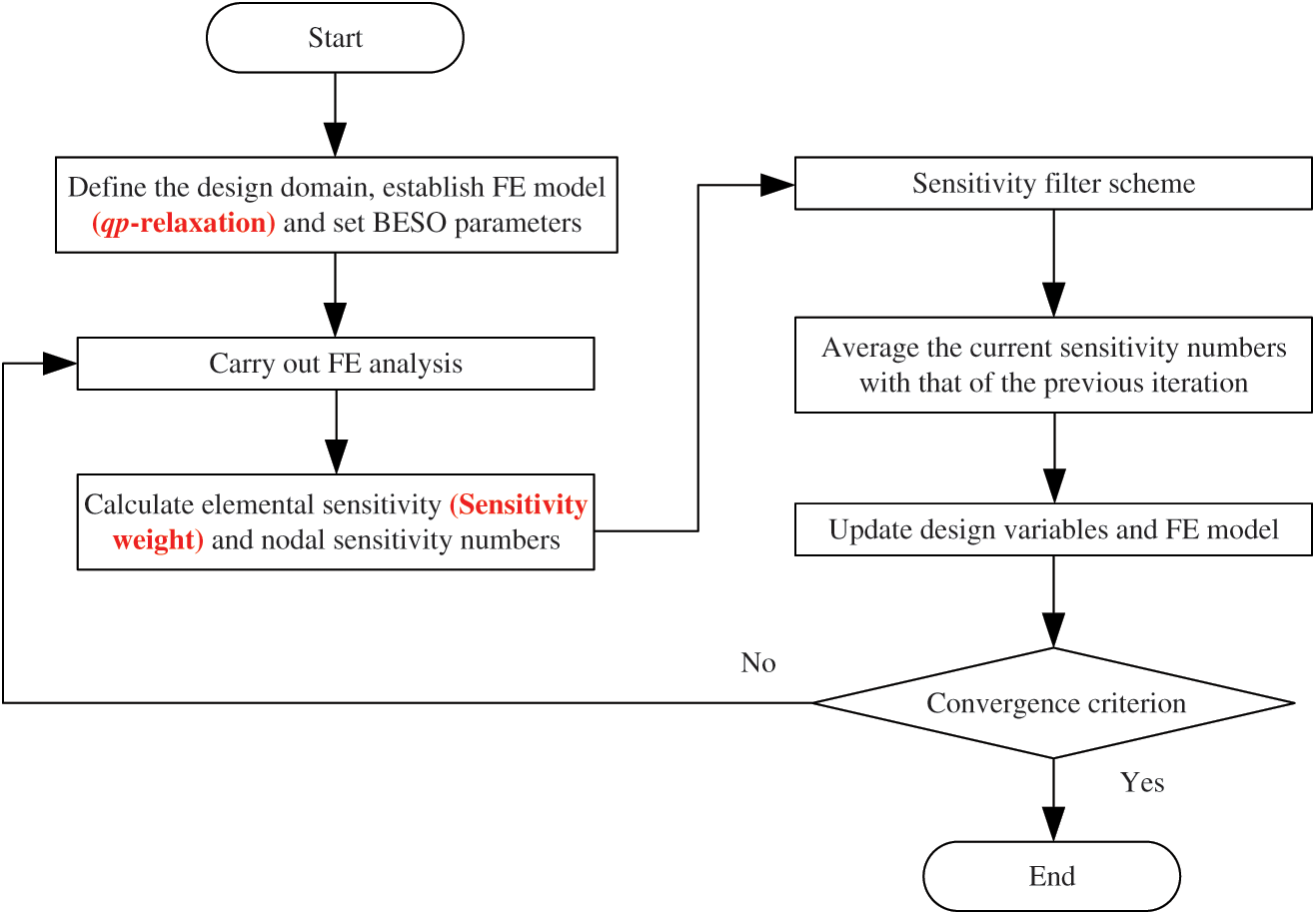
Figure 1: Flowchart of the conventional BESO method (black words only) and the improved BESO method (includes red words)

It is noted that to make the BESO can be applied to the stress-based topology optimization, Xia et al. [23] modified Steps 3–6 and Liu et al. [20] modified Steps 1–5, respectively.

2.2 Problem Statement

2.2.1 Global Stress Measure

Aggregation functions can aggregate large amounts of stress values to a global stress measure which approximates the maximum stress value [17,23]. This global stress measure has adequate smoothness so that the optimization algorithm could perform well [17]. p-norm function is used in this study

where denotes the global stress measure and denotes the von Mises stress at the centroid of the ith element. pn denotes the stress norm parameter. approaches to the average stress value when pn tends to one and approaches to the maximum stress value when pn tends to infinity. An appropriate stress norm parameter can balance the smoothness of the p-norm function and the approximation for the maximum stress value in the structure [17,23]. The determination of pn will be discussed in Section 3.

The von Mises stress can be expressed as follows:

where denotes the stress vector of centroid of ith element. is the stress coefficient matrix. For plane stress case, .

2.2.2 Optimization Formulation

With the global stress measure defined above and the common used volume constraint in BESO, the optimization formulation is stated as follows:

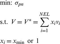
where V denotes the volume fraction of the optimal design. To avoid the singularity of the global stiffness matrix and re-meshing, in this study.

2.3 qp-Relaxation

Numerical experiments show that the smoothness of the global stress measure is not enough to obtain a reliable solution in the conventional BESO framework. To add more smoothness to the objective function, this study adopts the qp-relaxation [17] rather than Ersatz material model used in [23]:

where and D0 denote the constitutive matrix of material for ith element and solid material, respectively. denotes the stress vector of centroid of ith element assigned with solid material. is the strain-displacement matrix. is the nodal displacement vector of ith element. p, q are constants, unless noted, p = 3, q = 0.5 in this study.

The material interpolation is used to avoid re-meshing and singularity of the stiffness matrix in this study. Stress interpolation in density-based methods is usually used to further penalize the intermediate densities with a q < 1 [17,21]. In the framework of BESO, stress interpolation was originally unnecessary because this method uses discrete design variables [20,23]. It serves to stabilize the optimization process in this study. The effect of different p and q on topology optimization will be discussed in Section 3.2.

2.4 Sensitivity Analysis

The derivative of with respect to xj can be expressed as Eq. (7) based on Eq. (2):

Based on the framework in [23], the detailed sensitivity analysis with introduced qp-relaxation is given in Appendix A. Finally, the derivative of with respect to xj can be expressed as

where and denote a global adjoint vector and the adjoint vector of jth element, respectively. denotes the stiffness matrix of jth element with solid material. and denote the global nodal displacement vector and the nodal displacement vector of jth element, respectively. The matrix relates and , i.e., .

If there is no stress interpolation, Eq. (8) can be expressed as

The effect of qp-relaxation on stress-based topology optimization will be discussed in Section 3.

2.5 Sensitivity Weight

BESO uses pure 0/1 design variables to obtain a black-and-white design which may result in large spatial stress gradient in the vicinity of the zig-zag edges. Thus, the sensitivity field has a large spatial gradient which deteriorates the convergence of the BESO method in stress-related topology optimization [17]. To overcome this issue, a sensitivity weight is added to the sensitivity formulation and this weight is defined as

where ni and denote the number of solid elements that ith element connected with in the current iteration and that of ith element connected with in the initial design.

This scheme can be illustrated in Fig. 2a. The number of solid elements that ith element connected with is four in the current iteration, and that of the ith element in the initial design is five. Based on Eq. (9), the sensitivity weight of ith element is 0.8. While the sensitivity weight of kth, mth, nth element is 0.875. Once this weight is introduced to the sensitivity formulation, the sensitivity numbers of elements located at the edges of the structure can be artificially reduced. They have a higher probability to be removed. The fewer solid elements an element is connected with, the lower sensitivity weight it has. For a prominent element, it has either big stress value (e.g., elements located in the vicinity of stress concentration area, ith and jth element shown in Fig. 2a) or small stress value (e.g., elements away from the load paths, ith element shown in Fig. 2b). The former is harmful and the latter is inefficient, thus the prominent element should be removed. This can be achieved by the proposed sensitivity weight scheme. Numerical experiment shows that sensitivity weight calculation can be done in an instant. Thus the additional computational cost can be neglected compared with the total optimization process.

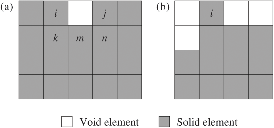
Figure 2: Illustration for sensitivity weight: (a) Prominent element in the stress concentration case. (b) Prominent element in the inefficient case

2.6 Sensitivity Numbers

In the framework of the BESO method, the statuses of elements are determined by the sensitivity numbers. Solid elements with lower sensitivity numbers are removed and void elements with higher sensitivity numbers are recovered. Elemental sensitivity number in this study is stated as product of the derivative of with respect to the design variable and the corresponding sensitivity weight, i.e.,

2.7 Numerical Implementation

As shown in Fig. 1, qp-relaxation and the proposed sensitivity weight scheme are embedded in the existing FE modelling and sensitivity calculation, respectively. These schemes are supplements to the conventional BESO framework rather than modifications. The implementation of BESO in this study is the same as that in [28] which has been summarized in Section 2.1. The implementation won’t be repeated here.

3  Numerical Examples

Three classical numerical examples and a practical engineering example are used to validate the proposed method. The Young’s modulus and the Poisson’s ratio are taken as 1.0 MPa and 0.3, respectively. The evolutionary volume ratio is 0.02 and the maximum admission volume ratio is 0.005. Due to the highly nonlinear stress behavior, the maximum stress value still fluctuates in a limited range when the specified volume fraction is achieved. Hence the conventional convergence criterion in [28] is inappropriate for stress minimization topology optimization. This study adopts the criterion proposed in [23], i.e., design with the lowest stress concentration is chosen after the specified volume fraction is achieved.

3.1 MBB Beam with a Notch

Firstly, a MBB beam with a pre-existing notch is analyzed. The dimension and boundary conditions are illustrated in Fig. 3. The thickness is 1.0 mm. Unless noted, all dimensions and stress value given in this paper are in mm and MPa, respectively. The design domain is meshed with 10,230 four-node plane stress elements. The average length of elements is about 1.0 mm and the filter radius is 3.0 mm. A vertical force is applied to the middle of the top edge. To avoid stress concentration, this force is distributed symmetrically over eleven adjacent nodes. The specified volume fraction V* is 0.4. The maximum von Mises stress in the structure appears at the notch of the beam and its value is .

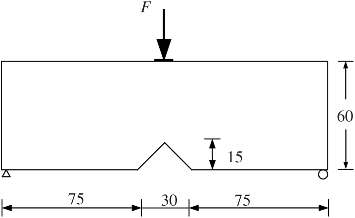
Figure 3: Problem definition for MBB beam

To illustrate the effect of qp-relaxation on stress-based topology optimization, this example was solved with and without qp-relaxation using stress norm parameter , respectively. The evolution histories of of designs are shown in Fig. 4. It is noted that the curves of in designs using qp-relaxation (blue line, denoted by relaxed) are more continuous than those of designs without qp-relaxation (red line, denoted by ) as shown in Figs. 4a, 4c and 4e. Without qp-relaxation, not only the designs of MBB example (as shown in Figs. 4b, 4d and 4f), but also all the examples employed in this study lose their integrities. Thus, this case will not be discussed in the rest of this study. In addition, as pn increases, relaxed approaches the maximum stress value in the structure.

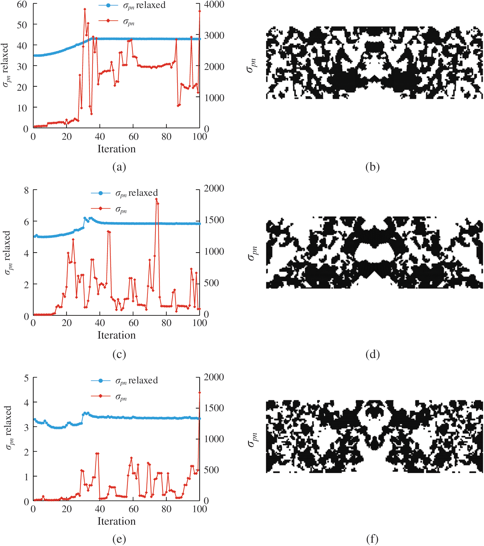
Figure 4: Comparison of evolution histories of of designs with and without qp-relaxation and designs obtained without qp-relaxation using , respectively. (a) pn = 2. (b) Design without qp-relaxation and pn = 2. (c) pn = 4. (d) Design without qp-relaxation and pn = 4. (e) pn = 6. (f) Design without qp-relaxation and pn = 6

The optimal designs obtained by the proposed method along with the stress distributions are shown in Fig. 5. To facilitate the comparison of stresses among different designs, unless noted, all stress distributions in this study use the same color scale. The scale has six equal range levels and ranges from blue (minimum stress) to red (maximum stress) as shown in Fig. 5f. Elements with stress values greater than 3.0 MPa are still marked in red. Fig. 5a is the compliance minimization design obtained by the conventional BESO method. Figs. 5b–5d are the optimal designs obtained with qp-relaxation and without sensitivity weight, the stress norm parameter , respectively. It is noted that the compliance minimization design is similar to the stress-based design with pn = 2 as shown in Fig. 5b. However, the maximum stress in Fig. 5a is 8.9 MPa which is much higher than that in Fig. 5b. Moreover, due to the mesh distortion in the vicinity of the constraint regions, the compliance value of compliance minimization design is also the largest among all of the optimal designs. It is clear from Figs. 5b–5d, with the increase of stress norm parameter pn, the lower edge is getting rounded, and hence, the stress concentration is reduced. Meanwhile, the compliance value increases. The optimal design with pn = 6 is similar to the result in [23] though the density filtering method was not used in this study.

Figure 5: Material and stress distributions of designs: (a) is compliance minimization design. (b–d) are stress-based designs with qp-relaxation and without sensitivity weight. (e) is stress-based design with qp-relaxation and sensitivity weight. (a) , , (b) pn = 2, , , (c) pn = 4, , , (d) pn = 6, , , (e) pn = 6, , , (f) the stress color scale

As stated earlier, a large pn makes the global stress measure tends to the maximum stress value in the design domain, i.e., the objective function of this study degenerates to the maximum stress function and loses smoothness [17]. This issue deteriorates the convergence of the BESO method. Thus, pn should be kept in an appropriate range. In this study, when pn equals to 8, the optimization process oscillates and designs in certain intermediate iterations lose their integrities. Thereby, pn is set to 6, when both qp-relaxation and sensitivity weight are employed. And the optimal design is shown in Fig. 5e. The boundary is smoother and the central part is wider than that of Fig. 5d, which helps to prevent the deflection of the structure. Therefore, the stress field is smoother and the compliance is lower than that in Fig. 5d. Moreover, the topology optimization process of the case in Fig. 5e converged at the ninetieth iteration while the case in Fig. 5d took ninety-seven iterations.

The evolution history of optimal design in Fig. 5e is shown in Fig. 6. In the early iterations, elements in the vicinity of the notch are removed and the lower edge is getting rounded which reduces the stress concentration. The topology and maximum stress value vary little between the fortieth iteration and the sixtieth iteration. The maximum von Mises stress is reduced by 33.4%.

Figure 6: Evolution history of topology together with stress field for the case of Fig. 5e

The computational efficiency in terms of design iterations of the proposed method is compared with the previous researches. The comparison is illustrated in Fig. 7. Though they differ in dimensions, they belong to the same kind of problem. Reference [17] reports that it takes 275 iterations using density-based method. Reference [22] does not report the number of iterations, based on the information given in the literature, it may take hundreds of iterations too. Both Xia’s method and the proposed method converge at about fiftieth iteration. These four studies all use adjoint method to carry out sensitivity computation. However, Le et al. [17] and Xia et al. [23] use sensitivity filtering method and density filtering method. Reference [22] has to calculate the sensitivities of Gauss points in each element. Therefore, in the same condition (i.e., the configuration of computer, mesh, FE solver, etc.), the efficiency of the proposed method is higher than that of the previous researches because this study uses sensitivity filtering method only.

Figure 7: MBB beam designs from different topology optimization methods and their typical number of iterations until convergence. (a) Le et al. [17] (density-based method, 275), (b) Picelli et al. [22] (LSM, unknown), (c) Xia et al. [23] (extended BESO, 50) (d) the present work (conventional BESO, 50)

3.2 L-Bracket Design

The second numerical example is the well-known L-bracket. The dimensions and boundary conditions are shown in Fig. 8. The thickness is 1.0 mm. The design domain is meshed with 25,600 four-node plane stress elements. The element length is 1.0 mm and is 3.0 mm. The top edge is well-fixed. A vertical force is distributed over eight nodes at the right edge of the L-bracket to avoid the stress concentration. The specified volume fraction is 0.4. The maximum stress value appears at the reentrant corner and its value is 1.87 MPa.

Figure 8: Problem definition for L-bracket

The optimal design obtained by compliance minimization is shown in Fig. 9a. The stress concentration area still exists in the structure. But compliance minimization design has the lowest compliance value. Figs. 9b–9d are the optimal designs obtained with qp-relaxation and without sensitivity weight, the stress norm parameter , respectively. The optimal designs obtained with lower pn are quite similar to the compliance minimization design. When pn equals to 6, the stress concentration is totally removed. The reentrant corner is replaced by a round corner. Moreover, similar with that in MBB example, when pn increases, the maximal stress value decreases and the compliance increases. Again, when pn takes a higher value than 8, it results in poor convergence due to the severe numerical oscillations.

Figure 9: Material and stress distributions of designs: (a) is compliance minimization design. (b–d) are stress-based designs with qp-relaxation and without sensitivity weight. (e) is stress-based design with qp-relaxation and sensitivity weight. (a) , , (b) pn = 2, , , (c) pn = 4, , , (d) pn = 6, , , (e) pn = 6, ,

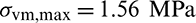Then, pn is set to 6 and both qp-relaxation and sensitivity weight scheme are employed. The optimal design is shown in Fig. 9e. The edges and stress distribution of the optimal design with sensitivity weight are a bit smoother than those without sensitivity weight shown in Fig. 9d. The proposed sensitivity weight scheme allows the thin members to be removed from the structure and strengthens the main members in the structure, leading to an evenly distributed stress field.

Based on the results mentioned above, it can be inferred that pn = 6 is an appropriate value to obtain a desirable solution. Thus, with pn = 6, the effect of different q and p on stress-based topology optimization has been discussed. The optimal designs with different p and q are shown in Fig. 10. It is clear that the optimal designs shown in Figs. 10a–10c are failed to obtain a reliable solution. Only the design shown in Fig. 10d with p = 3 and q = 0 is acceptable. Configuration in Fig. 10d is similar to that shown in Fig. 9d with p = 3 and q = 0.5 except for the thinner members. This indicates that the penalization factors for material interpolation scheme are crucial to a reliable solution in the framework of the conventional BESO method. When q = 0, Eq. (10) degenerates to a similar form with that in [23]. However, the raw elemental sensitivity numbers of void elements are set to zero in [23]. Though Xia et al. [23] used the so-called soft-kill BESO method [33], the stress values of void elements were not taken into account. Thus, it is deduced that these two factors are responsible for the poor convergence of the method proposed in [23] in the framework of the conventional BESO method. These numerical errors lead to the need for the density filtering method and other modifications to the conventional BESO method.

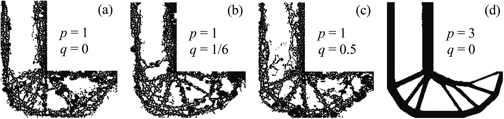
Figure 10: Optimal designs with different combinations of p and q. (a) p and q used in [23]. (b) p and q used in [17]. (c) p and q used in present work. (d) p and q used in present work

The evolution history of the optimal design in Fig. 9e is shown in Fig. 11. At the early stage of the optimization, the stress concentration region is removed and the maximum stress in the structure decreases to 1.36 MPa. In the twentieth iteration, the optimized structure has a minimal stress value 1.17 MPa, the lowest during the optimization. As the optimization process proceeds, the maximum stress increases slowly since the volume fraction continues to decrease. The volume fraction holds constant after the fortieth iteration. The maximum stress value fluctuates between 1.4 and 1.6 MPa because of the highly nonlinear stress behavior though the material distribution is almost unchanged. Finally, the maximum stress value in eighty-second iteration is 1.56 MPa which is reduced by 16.58% compared to that of the initial design. The case without sensitivity weight scheme in Fig. 9d took ninety iterations. The proposed method with sensitivity weight scheme exhibits a higher computational efficiency compared to that without sensitivity weight scheme.

Figure 11: The evolutionary history of topology together with stress field for the case of Fig. 9e

The optimal design obtained by the proposed method is similar to those in [17,22,23] as shown in Fig. 12. Compared with the density-based method or LSM, optimization in this study ends in fifty iterations instead of hundreds of iterations. Compared with the design in [23], density filtering method is not necessary for the proposed method. Therefore, under the same conditions (i.e., configuration of computer, FE solver, mesh, etc.), the proposed method is more efficient than the method in [23], the density-based method and the LSM.

Figure 12: L-bracket designs from different topology optimization methods and their typical number of iterations until convergence. (a) Le et al. [17] (density-based method, 70), (b) Picelli et al. [22] (LSM, 200–900), (c) Xia et al. [23] (extended BESO, 50) (d) the present work (conventional BESO, 50)

3.3 3D L-Bracket Design

To demonstrate the validity of the proposed method for 3D problem setting, 3D L-bracket is used and is obtained by extruding the aforementioned 2D L-bracket 100 mm. The dimension and boundary conditions are shown in Fig. 13. The top face of the L-bracket is totally constrained. The design domain is discretized by 40000 uniform cubic elements whose size is 4 mm. A vertical force is distributed over four rows of elements to avoid the stress concentration. The specified volume fraction is 0.3. is set to 8 mm. The maximum stress value appears at the reentrant corner and its value is 1.73 MPa.

Figure 13: Problem definition for 3D L-bracket

The optimal design obtained by compliance minimization optimization is shown in Fig. 14a. Compliance minimization design has the lowest compliance value and the largest maximum stress value, they are 600.7 J and 3.25 MPa, respectively. Figs. 14b–14d are the optimal designs obtained with qp-relaxation and without sensitivity weight, the stress norm parameter , respectively. When pn increases, the stress concentration is gradually reduced. The maximum stress values of designs in Figs. 14b–14d are 2.94, 2.46 and 2.3 MPa, respectively. The compliance increases from 621.7 to 655.5 J when pn increases from six to seven. But, the compliance decreases when pn increases from seven to eight. Moreover, it is noted that the profile of the optimal design in Fig. 14d is similar to the 2D case shown in Fig. 9d. The inner boundary is rounded too. However, it indicates that, to obtain a desirable design, the values of stress norm parameter pn are different for 2D and 3D problem settings. And in the 3D space, it exhibits a special topology which demonstrates that topology optimization could create innovative design.

Figure 14: Material and stress distributions of designs: (a) is compliance minimization design. (b–d) are stress-based designs with qp-relaxation and without sensitivity weight. (e) is stress-based design with qp-relaxation and sensitivity weight. (a) , , (b) pn = 6, , , (c) pn = 7, , , (d) pn = 8, , , (e) pn = 8, ,

Then pn is set to 8 and both qp-relaxation and sensitivity weight scheme are used. The optimal design is shown in Fig. 14e. It is noted that the stress field is evenly distributed though the topology is similar to that shown in Fig. 14d. Compliance and maximum stress of the design shown in Fig. 14e are a bit smaller than those in Fig. 14d.

The evolution history of the case in Fig. 14e is shown in Fig. 15. It is noted that the maximum stress value increases a lot in the first iteration since elements located at the reentrant corner are removed which leads to sharper edges. Subsequently, the maximum stress value decreases gradually. After the thirtieth iteration, it increases again. After the sixtieth iteration, the volume fraction holds constant and the maximum stress value fluctuates in a limited range. Finally, the optimization converges at the ninety-first iteration while the case in Fig. 14d takes ninety-three iterations to converge. It is concluded that the proposed sensitivity weight scheme not only distributes the stress field evenly and smooths the boundary, but also improves the computational efficiency.

Figure 15: The evolution history of topology together with stress field for the case of Fig. 14e

In this case, a refined mesh could more accurately evaluate the stress field, but the FE analysis and sensitivity computation will be expensive. This study aims to propose an applicable stress minimization topology optimization method and the results demonstrate that even a coarser mesh can get a desirable solution.

3.4 Suspension of Off-Road Truck Cab

The last example is a suspension of an off-road truck cab. Two suspensions mounting on the chassis support two frame rails under the floor of the cab and enable the cab tilts around the y-axis shown in Fig. 16a. Therefore, strength of the suspension is important for structural safety. Due to the symmetry of the loads and structure, a half model with 57 253 eight-node hexahedron elements is used for topology optimization as shown in Fig. 16b, where the red area represents the non-design domain and the blue area represents the design domain. The dimensions of the half model are shown in Appendix B. (Fig. B.1). All of the elements have a length of about 2 mm. This suspension is made out of steel. The Young’s modulus is 210 GPa, the Poisson’s ratio is 0.3. All of the freedoms of centers of hole A and hole B are constrained. A vertical load , representing the weight the suspension should support, is applied to the center of hole C. To the symmetry plane, the translational degrees of freedom in y-axis and the rotational degrees of freedom in x- and z-axis are constrained. The specified volume fraction is 0.2 and is 4.0 mm. Based on the conclusion of the 3D L-bracket, pn is set to 8. The maximum stress value of the initial design appears in the vicinity of hole A and its value is 31.1 MPa.

Figure 16: Illustration and problem definition of suspension. (a) Illustration of suspension. (b) Problem definition of suspension

This example also solved by commercial code, Altair Optistruct, and the problem was formulated to minimize the compliance of the suspension and subject to the same volume constraint [34]. The result is shown in Fig. 17a. The optimal designs obtained by the proposed method without and with sensitivity weight scheme are shown in Figs. 17b and 17c, respectively.

Figure 17: Optimal designs and stress contours of suspension. (a) Altair Optistruct (elements with density greater than 0.5 in the final iteration is saved and treated as solid elements). (b) Material distribution and stress contour of design obtained without sensitivity weight. (c) Material distribution and stress contour of design obtained with sensitivity weight

It is clear that boundaries of designs obtained by stress-based optimization are smoother than that obtained by the compliance minimization optimization. The reentrant corners of the initial design are replaced by arc shaped structures. The stress-based designs shown in Figs. 17b and 17c evenly distribute the stress fields and the maximal stresses are 35.1 and 30.8 MPa, respectively, which is lower than 58.15 MPa in Fig. 17a. Notably, the optimal design shown in Fig. 17c that obtained with sensitivity weight scheme is totally different and its boundary is smoother than that shown in Fig. 17b. Stress level shown in Fig. 17c is lower than that shown in Fig. 17b.

The evolution histories of maximal stress value of cases in Figs. 17b and 17c are shown in Fig. 18. Though, both curves fluctuate, they capture the trend of the maximum stress values. At the beginning, the maximal stress value in the structure decreases. Then, the maximal stress value increases gradually when the volume of the structure is less than a certain value. When the volume achieves the specified volume, the maximal stress values stay in a limited range. It is clear that the iteration process with sensitivity weight (red line, denoted by ) is more stable than that without it (green line, denoted by ). Thus, in summary, the design in Fig. 17c is better. The entire design for the case of Fig. 17c is shown in Fig. 19.

Figure 18: Evolution history of maximal stress with and without sensitivity weight

Figure 19: Entire design for the case of Fig. 17c from different perspectives

4  Conclusions

This study proposes a stress minimization topology optimization method for continuum structures based on the conventional BESO method. In the proposed method, qp-relaxation is introduced to circumvent the poor convergence of the conventional BESO method on stress-based topology optimization. A new sensitivity weight scheme is used to further stabilize the optimization process. The improved BESO method is applied to four 2D and 3D numerical examples. The optimal designs agree well with those reported in the literature. Moreover, the stress norm parameter pn and the penalization factors p and q are crucial to reliable solutions. Finally, the proposed method is more efficient than the previous BESO method, the density-based method and the LSM under the same conditions. The proposed method is an efficient stress minimization topology optimization method and could be generalized to multi-constrained or multi-objective topology optimization involving other criteria, e.g., displacement and frequency.

Funding Statement: This work was supported by National Natural Science Foundation of China [Grant No. 51575399]; and the National Key Research and Development Program of China [Grant No. 2016YFB0101602].

Conflicts of Interest: The authors declare that they have no conflicts of interest to report regarding the present study.

References

 1.  Bendsoe, M. P., Kikuchi, N. (1988). Generating optimal topologies in structural design using a homogenization method. Applied Mechanics and Engineering, 71(2), 197–224. DOI 10.1016/0045-7825(88)90086-2. [Google Scholar] [CrossRef]

 2.  Costa, G., Montemurro, M., Pailhes, J. (2019). Minimum length scale control in a NURBS-based SIMP method. Computer Methods in Applied Mechanics and Engineering, 354(9), 963–989. DOI 10.1016/j.cma.2019.05.026. [Google Scholar] [CrossRef]

 3.  Zhang, W., Zhong, W., Guo, X. (2014). An explicit length scale control approach in SIMP-based topology optimization. Computer Methods in Applied Mechanics and Engineering, 282, 71–86. DOI 10.1016/j.cma.2014.08.027. [Google Scholar] [CrossRef]

 4.  Wang, F., Lazarov, B. S., Sigmund, O., Jensen, J. S. (2014). Interpolation scheme for fictitious domain techniques and topology optimization of finite strain elastic problems. Computer Methods in Applied Mechanics and Engineering, 276, 453–472. DOI 10.1016/j.cma.2014.03.021. [Google Scholar] [CrossRef]

 5.  Wang, M. Y., Wang, X., Guo, D. (2003). A level set method for structural topology optimization. Computer Methods in Applied Mechanics and Engineering, 192(1), 227–246. DOI 10.1016/S0045-7825(02)00559-5. [Google Scholar] [CrossRef]

 6.  Zong, H., Liu, H., Ma, Q., Tian, Y., Zhou, M. et al. (2019). VCUT level set method for topology optimization of functionally graded cellular structures. Computer Methods in Applied Mechanics and Engineering, 354, 487–505. DOI 10.1016/j.cma.2019.05.029. [Google Scholar] [CrossRef]

 7.  Luo, Z., Zhang, N., Wu, T. (2012). Design of compliant mechanisms using meshless level set methods. Computer Modeling in Engineering & Sciences, 85(4), 299–328. DOI 10.3970/cmes.2012.085.299. [Google Scholar] [CrossRef]

 8.  Xie, Y. M., Steven, G. P. (1993). A simple evolutionary procedure for structural optimization. Computers & Structures, 49(5), 885–896. DOI 10.1016/0045-7949(93)90035-C. [Google Scholar] [CrossRef]

 9.  Xie, Y. M., Steven, G. P. (1996). Evolutionary structural optimization for dynamic problems. Computers & Structures, 58(6), 1067–1073. DOI 10.1016/0045-7949(95)00235-9. [Google Scholar] [CrossRef]

10. Guo, X., Zhang, W., Zhang, J., Yuan, J. (2016). Explicit structural topology optimization based on moving morphable components (MMC) with curved skeletons. Computer Methods in Applied Mechanics and Engineering, 310, 711–748. DOI 10.1016/j.cma.2016.07.018. [Google Scholar] [CrossRef]

11. Zhang, W., Li, D., Zhang, J., Guo, X. (2016). Minimum length scale control in structural topology optimization based on the Moving Morphable Components (MMC) approach. Computer Methods in Applied Mechanics and Engineering, 311, 327–355. DOI 10.1016/j.cma.2016.08.022. [Google Scholar] [CrossRef]

12. Wu, J., Clausen, A. T., Sigmund, O. (2017). Minimum compliance topology optimization of shell-infill composites for additive manufacturing. Computer Methods in Applied Mechanics and Engineering, 326, 358–375. DOI 10.1016/j.cma.2017.08.018. [Google Scholar] [CrossRef]

13. Zhang, S., Li, P., Zhong, Y., Xiang, J. (2014). Structural topology optimization based on the level set method using COMSOL. Computer Modeling in Engineering & Sciences, 101(1), 17–31. DOI 10.3970/cmes.2014.101.017. [Google Scholar] [CrossRef]

14. Yu, C., Wang, Q., Mei, C., Xia, Z. (2020). Multiscale isogeometric topology optimization with unified structural skeleton. Computer Modeling in Engineering & Sciences, 122(3), 779–803. DOI 10.32604/cmes.2020.09363. [Google Scholar] [CrossRef]

15. Nabaki, K., Shen, J., Huang, X. (2019). Stress minimization of structures based on bidirectional evolutionary procedure. Journal of Structural Engineering, 145(2), 4018256. DOI 10.1061/(ASCE)ST.1943-541X.0002264. [Google Scholar] [CrossRef]

16. Nabaki, K., Shen, J., Huang, X. (2019). Evolutionary topology optimization of continuum structures considering fatigue failure. Materials & Design, 166, 107586. DOI 10.1016/j.matdes.2019.107586. [Google Scholar] [CrossRef]

17. Le, C. H., Norato, J. A., Bruns, T. E., Ha, C., Tortorelli, D. A. (2010). Stress-based topology optimization for continua. Structural and Multidisciplinary Optimization, 41(4), 605–620. DOI 10.1007/s00158-009-0440-y. [Google Scholar] [CrossRef]

18. Xia, Q., Shi, T., Liu, S., Wang, M. Y. (2012). A level set solution to the stress-based structural shape and topology optimization. Computers & Structures, 90(1), 55–64. DOI 10.1016/j.compstruc.2011.10.009. [Google Scholar] [CrossRef]

19. Duysinx, P., Bendsoe, M. P. (1998). Topology optimization of continuum structures with local stress constraints. International Journal for Numerical Methods in Engineering, 43(8), 1453–1478. DOI 10.1002/(SICI)1097-0207(19981230)43:8¡1453::AID-NME480¿3.0.CO;2-2. [Google Scholar] [CrossRef]

20. Liu, B., Guo, D., Jiang, C., Li, G., Huang, X. (2019). Stress optimization of smooth continuum structures based on the distortion strain energy density. Computer Methods in Applied Mechanics and Engineering, 343, 276–296. DOI 10.1016/j.cma.2018.08.031. [Google Scholar] [CrossRef]

21. Luo, Y., Wang, M. Y., Kang, Z. (2013). An enhanced aggregation method for topology optimization with local stress constraints. Computer Methods in Applied Mechanics and Engineering, 254, 31–41. DOI 10.1016/j.cma.2012.10.019. [Google Scholar] [CrossRef]

22. Picelli, R., Townsend, S., Brampton, C. J., Norato, J. A., Kim, H. A. (2018). Stress-based shape and topology optimization with the level set method. Computer Methods in Applied Mechanics and Engineering, 329, 1–23. DOI 10.1016/j.cma.2017.09.001. [Google Scholar] [CrossRef]

23. Xia, L., Zhang, L., Xia, Q., Shi, T. (2018). Stress-based topology optimization using bi-directional evolutionary structural optimization method. Computer Methods in Applied Mechanics and Engineering, 333, 356–370. DOI 10.1016/j.cma.2018.01.035. [Google Scholar] [CrossRef]

24. Paris, J., Navarrina, F., Colominas, I., Casteleiro, M. (2010). Block aggregation of stress constraints in topology optimization of structures. Advances in Engineering Software, 41(3), 433–441. DOI 10.1016/j.advengsoft.2009.03.006. [Google Scholar] [CrossRef]

25. Cheng, G., Guo, X. (1997). -relaxed approach in structural topology optimization. Structure Optimization, 13(4), 258–266. DOI 10.1007/BF01197454. [Google Scholar] [CrossRef]

26. Bruggi, M. (2008). On an alternative approach to stress constraints relaxation in topology optimization. Structural and Multidisciplinary Optimization, 36(2), 125–141. DOI 10.1007/s00158-007-0203-6. [Google Scholar] [CrossRef]

27. Zhang, S., Gain, A. L., Norato, J. A. (2017). Stress-based topology optimization with discrete geometric components. Computer Methods in Applied Mechanics and Engineering, 325, 1–21. DOI 10.1016/j.cma.2017.06.025. [Google Scholar] [CrossRef]

28. Huang, X., Xie, Y. M. (2007). Convergent and mesh-independent solutions for the bi-directional evolutionary structural optimization method. Finite Elements in Analysis and Design, 43(14), 1039–1049. DOI 10.1016/j.finel.2007.06.006. [Google Scholar] [CrossRef]

29. Huang, X., Zuo, Z. H., Xie, Y. M. (2010). Evolutionary topological optimization of vibrating continuum structures for natural frequencies. Computers & Structures, 88(5), 357–364. DOI 10.1016/j.compstruc.2009.11.011. [Google Scholar] [CrossRef]

30. Simonetti, H. L., Almeida, V. S., Neves, F. D. A. D. (2018). Smoothing evolutionary structural optimization for structures with displacement or natural frequency constraints. Engineering Structures, 163, 1–10. DOI 10.1016/j.engstruct.2018.02.032. [Google Scholar] [CrossRef]

31. Zuo, Z. H., Xie, Y. M. (2014). Evolutionary topology optimization of continuum structures with a global displacement control. Computer-Aided Design, 56, 58–67. DOI 10.1016/j.cad.2014.06.007. [Google Scholar] [CrossRef]

32. Da, D., Xia, L., Li, G., Huang, X. (2018). Evolutionary topology optimization of continuum structures with smooth boundary representation. Structural and Multidisciplinary Optimization, 57(6), 2143–2159. DOI 10.1007/s00158-017-1846-6. [Google Scholar] [CrossRef]

33. Huang, X., Xie, Y. M. (2010). Evolutionary topology optimization of continuum structures: Methods and applications. Chichester, England: John Wiley & Sons, Ltd. [Google Scholar]

34. OptiStruct. (2016). Users Manual v/. 14.0. Troy, MI: Altair Engineering Inc. [Google Scholar]

35. Logan, D. L. (2012). A first course in the finite element method. 5th ed. Stamford, CT, USA: Cencage Learning. [Google Scholar]

Appendix A. Sensitivity analysis

The derivative of with respect to xj can be calculated by the chain rule and expressed as follows

According to the definition in Eqs. (3) and (6), the derivative of with respect to can be written as

And the derivative of with respect to xj can be expressed as follows:

It is noted that if , the first term in the right side of Eq. (A.3) is zero.

In order to obtain the derivative of , a matrix that relates and the global nodal displacement vector u is introduced

The equilibrium function of the structure subjected to a constant static load is

Differentiating both sides of Eq. (A.5), the derivative of u with respect to xj equals

Substituting Eqs. (A.4) and (A.6) into the Eq. (A.3), the sensitivity of can be further expressed as:

Substituting Eqs. (A.2) and (A.7) into Eq. (A.1), the sensitivity of with respect to xj can be further written as:

Substituting Eq. (A.8) into Eq. (7), one can obtain

An adjoint vector is introduced to calculate the second term in the parentheses of Eq. (A.9)

Thus Eq. (A.9) can be simplified as

The global stiffness matrix is assembled based on proper superposition of the individual elemental stiffness matrix [35]. This process can be described as

where denotes the stiffness matrix of ith element.

The stiffness matrix of jth element can be stated as:

where denotes the stiffness matrix of jth element with solid material. denotes the jth element domain.

It is noted that is independent from any other design variables, hence the derivative of K with respect to xj equals

Substituting Eq. (A.14) into Eq. (A.11), the derivative of with respect to xj can be further simplified as

Appendix B. Dimensions of the suspension

Figure B.1: Dimensions of suspension. (a) Side view. (b) Top view

This work is licensed under a Creative Commons Attribution 4.0 International License, which permits unrestricted use, distribution, and reproduction in any medium, provided the original work is properly cited.