Computer Modeling in Engineering & Sciences

DOI: 10.32604/cmes.2021.012730

ARTICLE

A Comparative Numerical Study of Parabolic Partial Integro-Differential Equation Arising from Convection-Diffusion

Kamil Khan1, Arshed Ali1,*, Fazal-i-Haq2, Iltaf Hussain3 and Nudrat Amir4

1Department of Mathematics, Islamia College, Peshawar, 25000, Pakistan
2Department of Mathematics, Statistics and Computer Science, The University of Agriculture, Peshawar, 25000, Pakistan
3Department of Basic Sciences & Islamiat, University of Engineering & Technology, Peshawar, 25000, Pakistan
4Department of Basic Sciences & Humanities, CECOS University of Information Technology and Emerging Sciences, Peshawar, 25000, Pakistan
*Corresponding Author: Arshed Ali. Email: arshad.ali@icp.edu.pk
Received: 10 July 2020; Accepted: 10 November 2020

1  Introduction

Partial integro-differential equations have been applied to model different physical phenomena in science and engineering such as heat conduction [1], reactor dynamics [2], flow in fractured biomaterials [3], electricity swaptions [4], financial option pricing [5], viscoelasticity [6], population dynamics [7], and convection-diffusion [8–11].

Convection-diffusion integro-differential equation has been used to model several important physical phenomena such as heat and mass transfer, flows in porous media, current density in fluids, and pollutant transport in atmosphere, streams, rivers and oceans (see [8,10,11] and the references therein).

PIDE models have been rarely solved analytically and their general solution is only obtained under restrictive conditions [12]. Due to such restrictive conditions the models become over simplified and also limit their physical relevance. Therefore, alternative approaches have been obtained for the solution of PIDEs including finite difference methods [13,14], finite element method [15], radial basis function collocation methods [16], spectral method [17], quasi-wavelet method [18], and spline methods [19–21].

This paper is devoted to comparative study of two efficient numerical techniques for solution of convection-diffusion parabolic PIDE [8,10] defined by:

with initial condition

boundary conditions

where the integral term is known as memory term, are known functions, and , is weakly singular kernel. The parameters c and d are positive constants which represent quantities of the convection and diffusion processes respectively. Different numerical techniques are developed to obtain the solution of the PIDE (1). Siddiqi et al. [8] employed cubic b-spline functions to spatial derivatives and Euler backward formula to time derivative to solve the PIDE (1). Ali et al. [9] constructed quartic B-spline collocation technique to obtain the solution of the PIDE (1). Fahim et al. [10] have solved (1) using product trapezoidal integration rule and sinc collocation method. Recently, Al-Humedi et al. [11] have solved (1) using cubic B-spline Galerkin method with quadratic weight function.

The cubic trigonometric B-spline methods are numerically accurate, computationally fast, consistent, and has ability to get the approximate solution at any point in the domain with more accuracy as compared to the conventional finite difference method which approximates solution at only selected points in the domain. In recent years solution of several partial differential equations have been found using these methods [22–28] due to special geometric features of trigonometric splines [22,29–31]. In 1964, Schoenberg [29] introduced piecewise trigonometric spline functions and founded the theory of locally supported trigonometric splines, named as trigonometric B-splines. It was derived that trigonometric spline can be written as linear combination of trigonometric B-splines. Lycche et al. [32] derived a recurrence relation using trigonometric B-splines divided differences for stable computation of trigonometric splines. They also formulated derivatives of trigonometric B-splines and provided an integral representation of trigonometric divided differences with trigonometric B-spline as kernel. Later on several other researchers have enhanced the theory of trigonometric B-splines by further developing many important properties such as C2 continuity, nonnegativity, partition of unity, smoothness, curve control and its analysis, and banded interpolation matrix (see [22,30,31] and the references therein). The first application of cubic trigonometric B-spline functions appeared in the literature in 2010 [33] when these functions were used for the solution of Two-point boundary value problem. In 2014, CTBS functions were extended for the solution of initial and boundary-value hyperbolic problems [22]. Recently, CBTS functions have been employed for the solution of PIDE problem [19,34]. The CTBS functions are also employed for the solution different problems which include Hunter Saxton equation [25], time fractional diffusion-wave equation [26], Fisher’s reaction-diffusion equations [28], non-conservative linear transport problems [27], Nonclassical diffusion problems [35], Hyperbolic telegraph equation [36], Fisher’s equations [37], and coupled Burgers’ equations [38].

In 1937, Frazer et al. [39] initiated the use of collocation method. This method is a special variant of the method of weighted residuals which uses dirac delta functions as weighting functions to minimize the residual. The main advantage of the collocation method is that as the number of collocation points increases, more points from the domain satisfy the functional equation. As a result approximate solution obtained by this method approaches to exact solution. Another advantage of this method is that using the dirac delta function makes computation of residual easy. The method is coupled with other methods such as Galerkin method, least squares method, Newton’s method, and finite difference method for the solution of various problems (see [22,40,41] and the references therein). In this paper, the first technique is developed by coupling CTBS functions with collocation procedure (CTBS-CT) for the solution of problem (1). The main advantage of this technique is that it reduces (1) to a tridiagonal system of linear equations which can be solved by an efficient tridiagonal solver.

The differential quadrature (DQ) method was projected as strong alternative of conventional methods i.e., finite difference and finite element methods. This method produces accurate numerical results with little computational effort as it uses smaller set of grid points while the conventional methods need relatively larger sets [42,43]. The DQ method was first introduced by Bellman et al. [44] in 1971, for approximating derivative of a sufficiently smooth function. The basic structure of DQ method is that it uses a weighted linear sum of functional values to approximate the function derivatives. The weighting coefficients play a key role since accuracy of the approximation depends on the accuracy of these coefficients. Initially Bellman and his co-researchers have developed two methods for determination of weighting coefficients [45]. However, the methods lead to ill-conditioned algebraic system for larger set of grid points. Shu [46] presented a systematic theoretical analysis and applications of earlier work about this method, and introduced two explicit approaches (i) a recurrence formula, and (ii) matrix multiplication, for computing the weighting coefficients of higher order derivatives to avoid the ill-conditioned system. The selection of grid points also effects accuracy of the DQ method and better accuracy was achieved using non-uniform and scattered grid points, and ghost points [34,43,47,48]. The DQ method is extended for the solution of various problems including Fisher’s reaction-diffusion equations [28], coupled viscous Burgers’ equations [38], space-dependent inverse heat problems [48], Kawahara equation [49], and shock wave simulations [50].

Recently, Korkmaz et al. [27] pioneered DQ method along with CTBS functions for the solution of second order advection-diffusion equation. Tasmir et al. [28] presented modified CTBS functions based DQ method for second order nonlinear Fisher’s reaction-diffusion equations. Kumar Singh et al. [38] extended the method for the solution of one and two dimensional coupled viscous Burgers’ equations. Arora et al. [51] developed a hybrid CTBS based DQ method for the solution of nonlinear Burgers’ equations. In this paper, the other technique is developed by coupling CTBS functions with differential quadrature (CTBS-DQ) approach. The key feature of this approach is that it reduces (1) to a system of ODEs which can be solved by any ODE solver.

Upto the best of our knowledge a comparative study of PIDE (1) using the proposed techniques has not been done. Moreover, solving PIDEs of the form (1) numerically have two major challenges in addition to discretization of temporal and spatial derivatives: the singular kernel and approximation of the memory term which also affect stability and accuracy of a numerical method.

Remaining work of the paper is arranged as follows: Section 2 shows development of the proposed methods through combination of CTBS functions with collocation and differential quadrature procedures. Section 3 analyzes stability of the present schemes. Section 4 shows numerical results of both methods including error norms, computational efficiency, conditioning, spectral radii, convergence and comparison with an existing method in order to establish the current approaches. Section 5 concludes the findings and outcomes of the paper.

2  The Proposed Methods

In order to develop, the proposed methods, consider the problem (1)–(3). The spatial domain is divided into N sub-intervals , of equal length by the nodes with and . Let , where is temporal step.

2.1 CTBS-CT

Taking in Eq. (1) and the temporal derivative is approximated by Euler backward formula which reduces Eq. (1) to the following form:

The integral part of Eq. (4) is approximated as below ([9]):

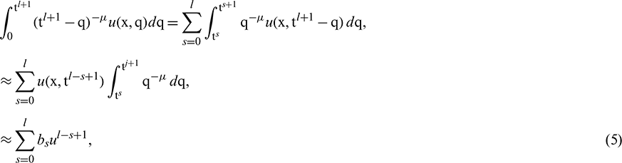
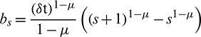where ul denotes and and as .

Putting Eq. (5) in Eq. (4), we get

where .

Simplifying Eq. (6), we get

where and .

Now collocating Eq. (7) at , we obtain

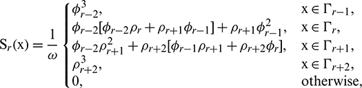
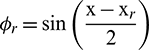
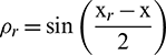
where . Next using CTBS functions , given in [22,23] to approximate .

Let

where

, , and .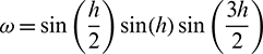

Lemma [22,33]: The values of , and at the node are obtained as:

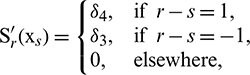
and

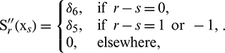
Then using Eq. (9), the function u and its derivatives at the rth node 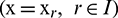can be expressed as

where ,

Thus by using (10) in (8) and combining like terms, we get

where , and

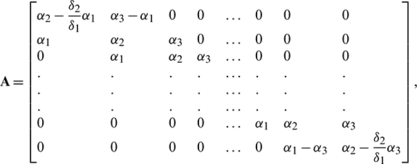
For r = 0 and N, Eq. (11) reduces to and respectively. After eliminating the parameters Cl+1 −1 and Cl+1N+1 using (10) and the boundary conditions (3), we get the linear system of N + 1 equations in N + 1 unknowns whose matrix form is as follows:

where

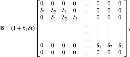
and

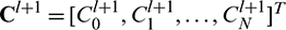
Eq. (12) can be re-written as

where and . The system Eq. (12) is solved using the efficient tridiagonal solver “Thomas Algorithm.”

2.2 CTBS-DQ

The DQ approach provides kth order derivative of the function from the values of at , as

where a(k)rs, are kth order weighting coefficients (WCs) which are determined by test functions. Different basis functions have been employed as test functions for determination of the WCs such as CTBS functions [27,38], polynomials [42], radial basis functions [48], cubic B-spline functions [49], and sinc functions [50]. In CTBS-DQ method we take the following test functions which are defined as modified CTBS functions [51]:

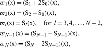
which form a basis in region .

Thus for each basis function , Eq. (14) gives

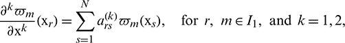
which leads to the following matrix form:

where 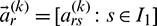, , 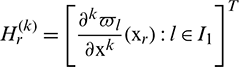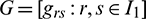and

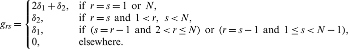
The weighting coefficients are obtained by solving the system (15) through the well known efficient tridiagonal solver “Thomas algorithm.” Now using (14) in (1) and taking to obtain the differential quadrature based technique,

The explicit time marching process for Eq. (16) is obtained as follows:

where . Using Eq. (5) in Eq. (17) and combining the like terms, we get

Eq. (18) leads to the following matrix form:

where

and , .

3  Stability Analysis

In this section we assess stability of the present schemes (13) and (19). Let en, un and represent error, exact solution and approximate solution at nth time level respectively, then . The error equation for the methods (13) and (19) is given by

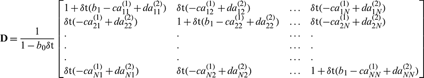
where D is the amplification matrix. The schemes (13) and (19) will be stable if (see [52] and Lax-Richtmyer condition for stability). This condition is equivalent to , where represents spectral radius of the matrix D [53] and is defined as 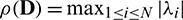and is an eigenvalue of D. The values of depend on and . Computational values of for different values of the parameters and are provided in the next section which show that the schemes (13) and (19) satisfy the condition of stability.

4  Test Problems

In this section three examples are taken from the literature [8] to validate the present approaches (13) and (19) for the solution of the problem (1)–(3) and comparison is also made with results obtained by cubic B-spline collocation method (CBSC) [8]. The methods are examined via error norms [8]. The schemes are also tested for convection and diffusion dominated problems via the Peclet number . High values of P lead to convection dominated problem while lower values of P lead to diffusion dominated problem [8]. Computations are carried out with Corei3, 2.4 GHz processor, 4 GB Ram, Matlab7.5 and computer run time (RT) is provided in seconds.

4.1 Problem 1

We take Eqs. (1)–(3) with convection-diffusion coefficients c = 0.1, d = 0.1 and elsewhere mentioned, and choose such that the exact solution is given by [8]

The conditions g, g1, g2 are found from Eq. (21). The error norms are obtained using the present methods (13) and (19) along with different values of the parameters number of nodes N, time step , time level M, convection and diffusion coefficients c, d, and which are reported in Tabs. 1–6. The effect of the convection and diffusion coefficient parameters c, d on the accuracy of both the methods are shown in Tab. 1. Computational efficiency RT of the methods are given in Tabs. 2 and 3 which shows that both the proposed methods are highly efficient. Numerical rate of convergence with respect to N and are provided in Tabs. 4 and 5, and it can be seen that the CTBS-CT has higher rate of convergence than the CTBS-DQ. However, the rate of convergence of CTBS-DQ becomes higher than that of CTBS-CT for larger values of spatial nodes N. From Tabs. 4–6, it can be noted that numerical values of for both methods satisfy the stability condition given in Section 3, whereas regarding CTBS-CT remains reasonably small. From Tab. 6, it can be noted that as the parameter decreases accuracy of the CTBS-DQ slightly increases as compared to the CTBS-CT. Furthermore, better accuracy of CTBS-CT than CBSC method [8] is evident from Tab. 7. The solution of (1) for cases of convection dominant and diffusion dominant problems are also provided in this table. It can also be seen from these tables that the CTBS-CT gives better results than the CTBS-DQ. Fig. 1 represents solutions obtained using CTBS-DQ and CTBS-CT at M = 1000. Fig. 2 displays errors in approximation obtained by the present methods. Fig. 3 shows the CTBS based solutions at different time levels. Fig. 4 represents condition numbers of system matrices of the methods. Fig. 5 compares convergence in space for the proposed methods.

Table 1: Error norms for different values of convection and diffusion coefficients using , M = 100, N = 100

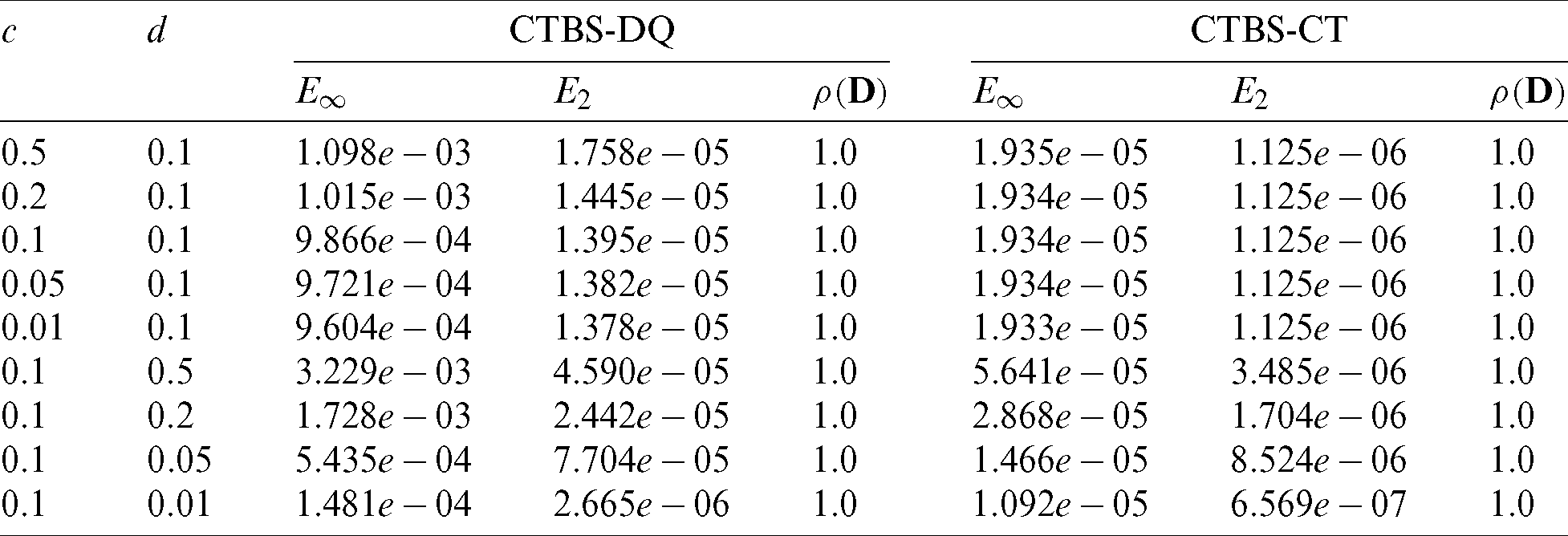
Table 2: Error norms vs. N using , M = 100

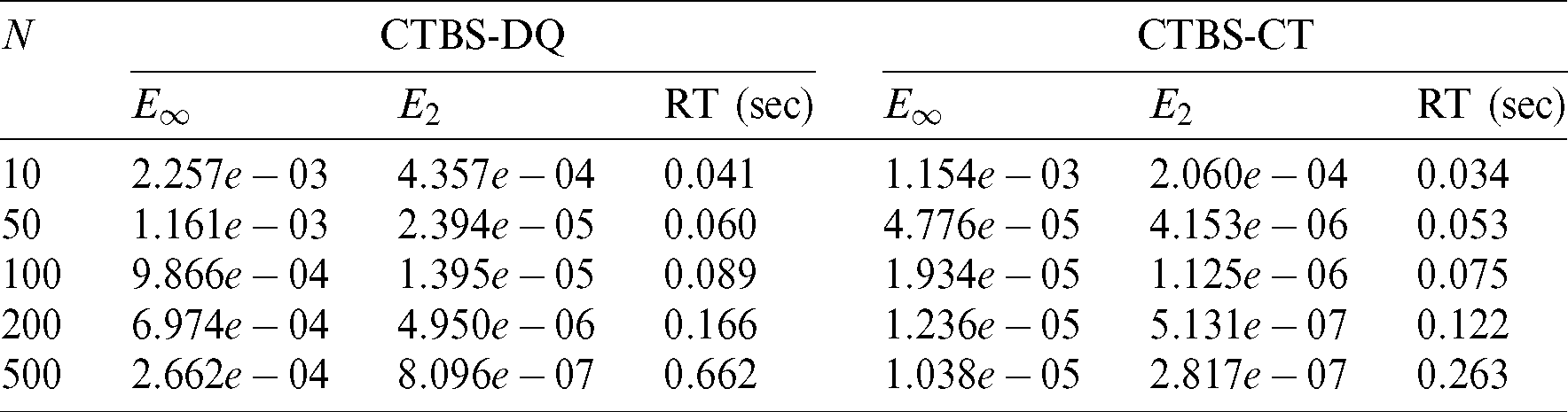
Table 3: Error norms at various time levels M using and N = 100

Table 4: Convergence in space using and M = 100

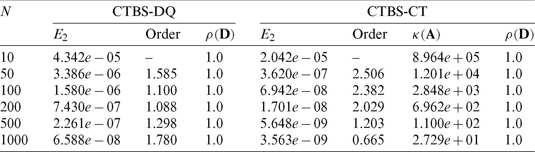
Table 5: Convergence in time using N = 100 and

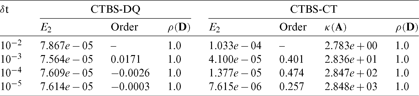
Table 6: Error norms vs. the parameter using , N = 100 and M = 100

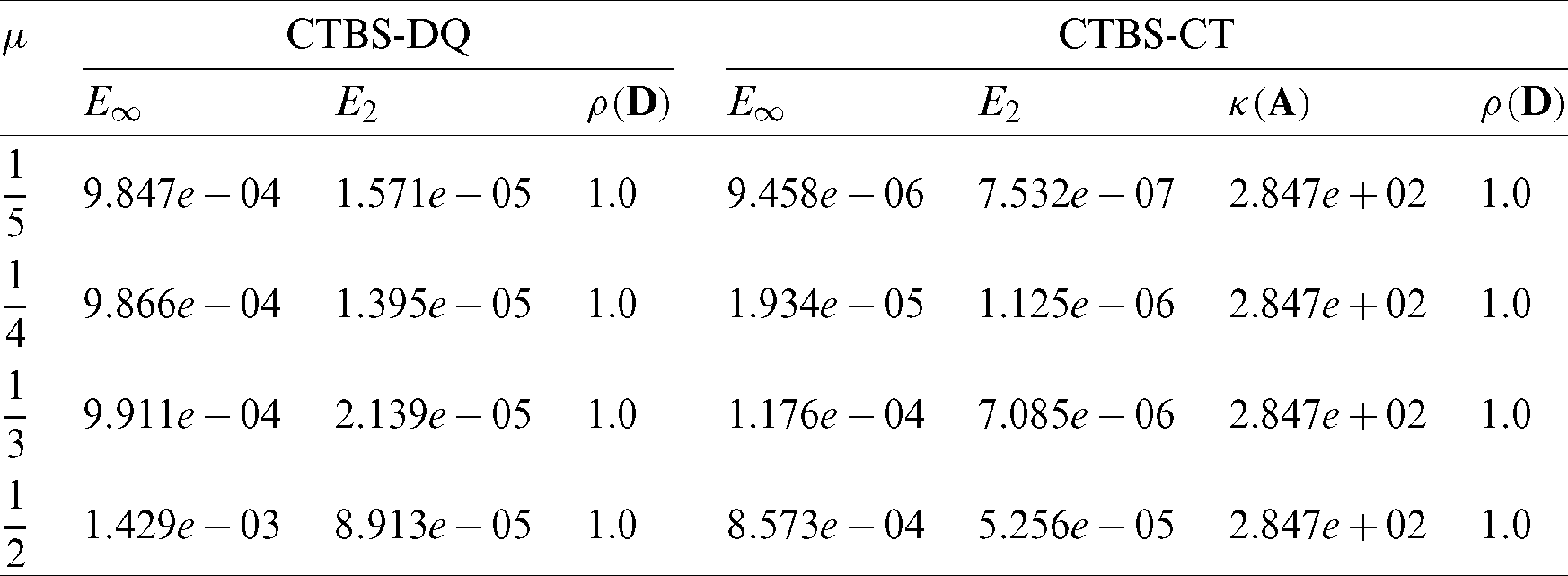
Table 7: Comparison of error norms with CBSC method [8],

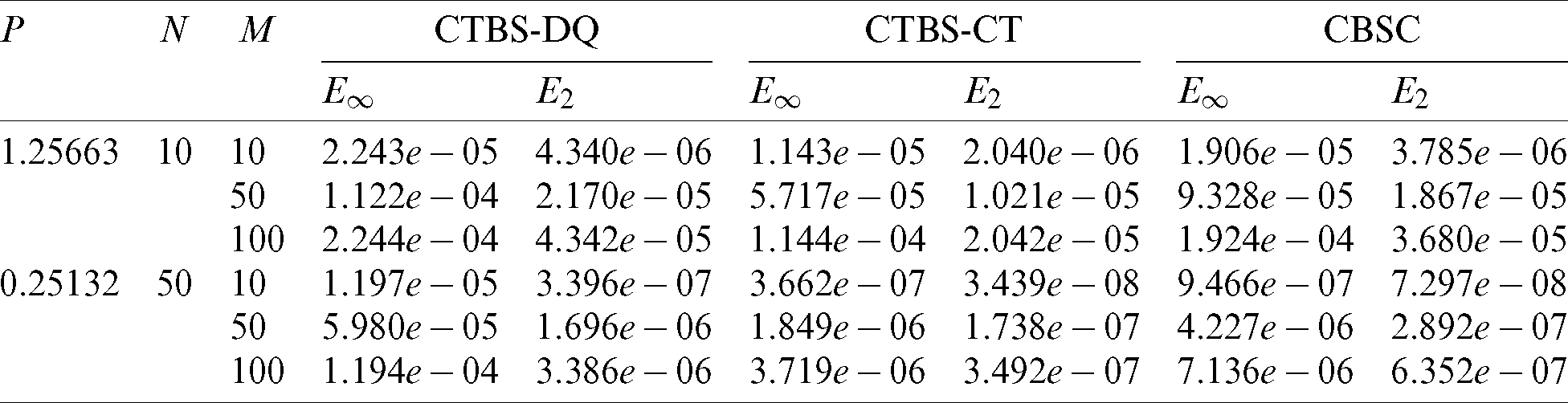
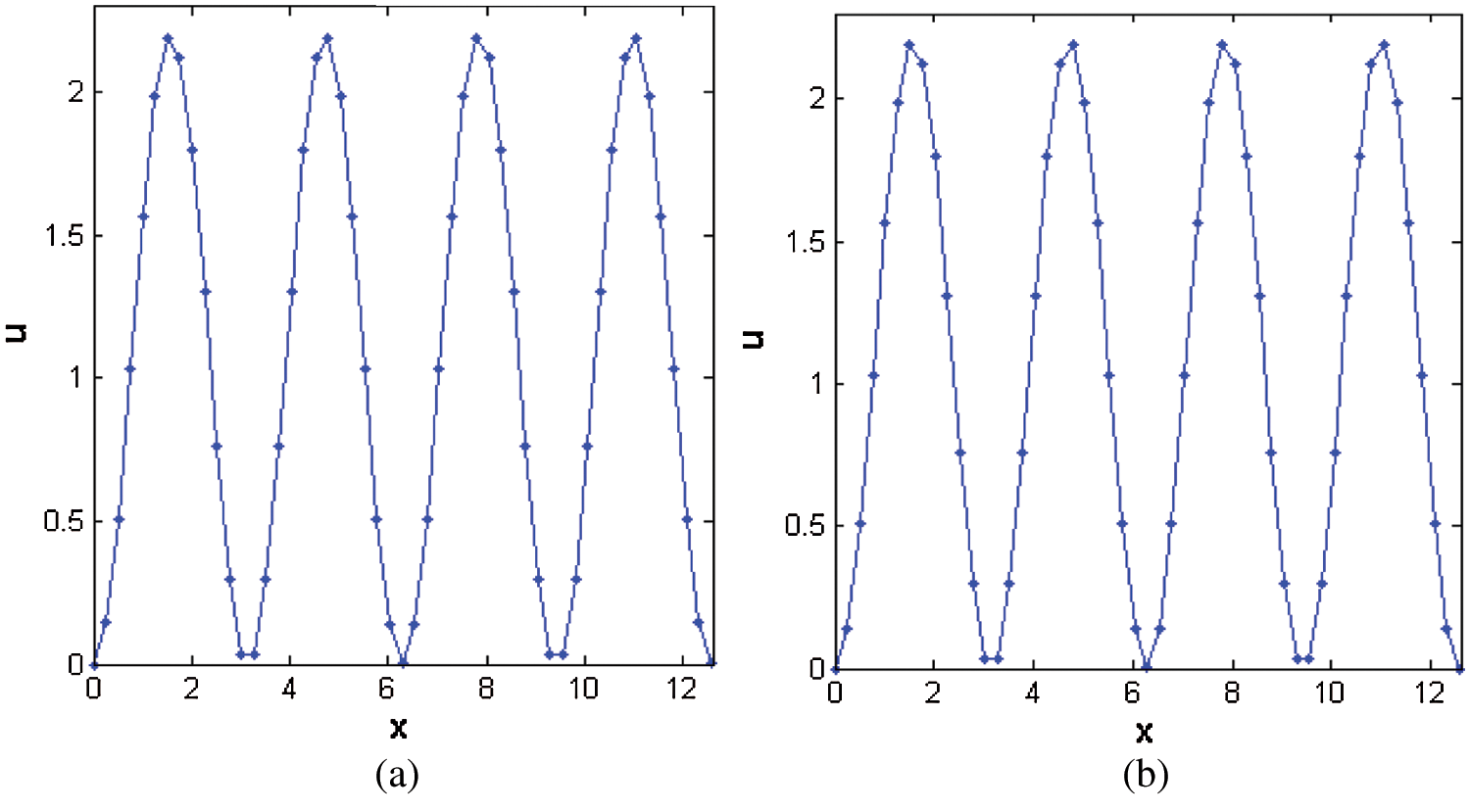
Figure 1: Numerical solutions obtained by (a) CTBS-DQ (b) CTBS-CT, using N = 50, , M = 1000, c = 0.1, d = 0.1,

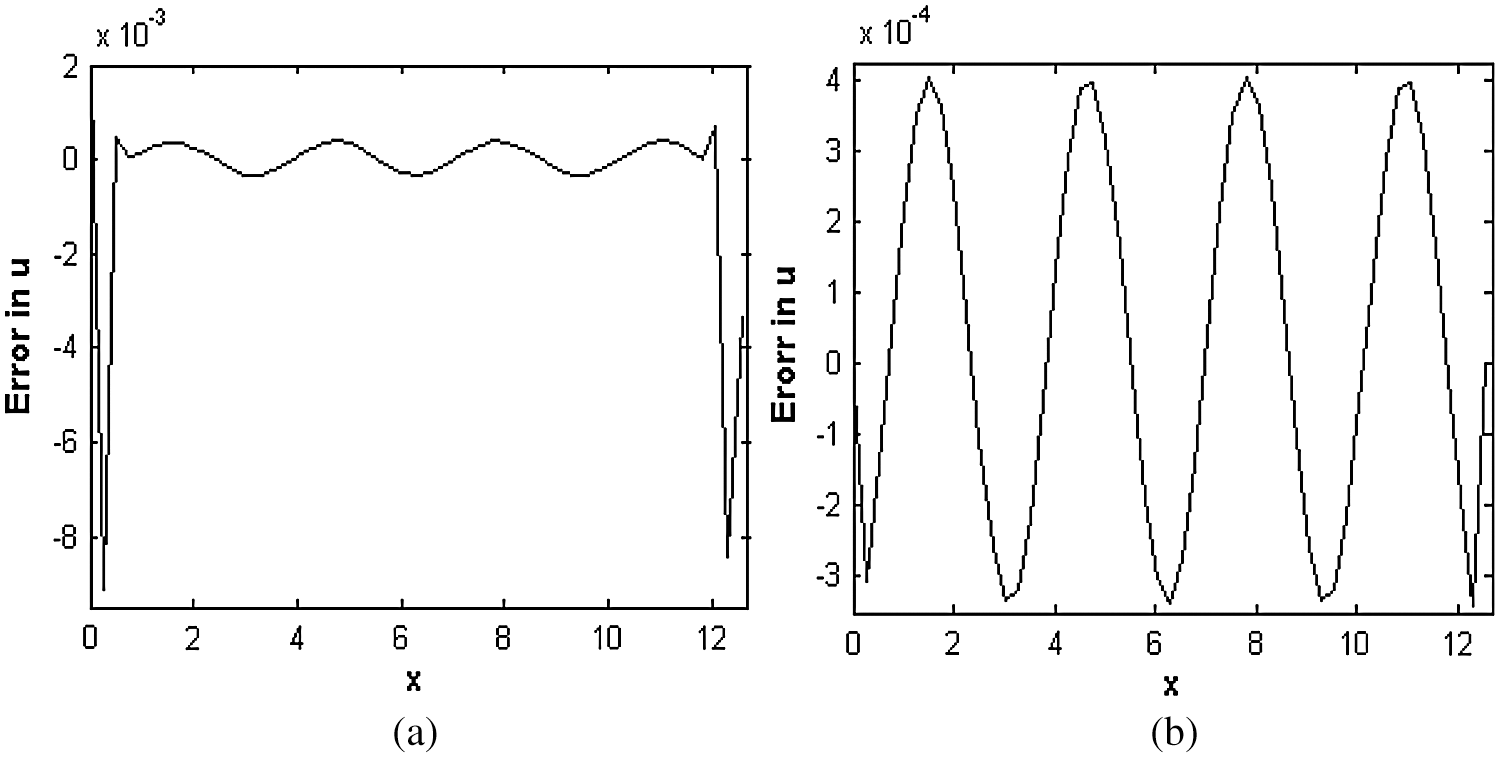
Figure 2: Error in numerical solutions obtained by (a) CTBS-DQ (b) CTBS-CT, using N = 50, , M = 1000, c = 0.1, d = 0.1,

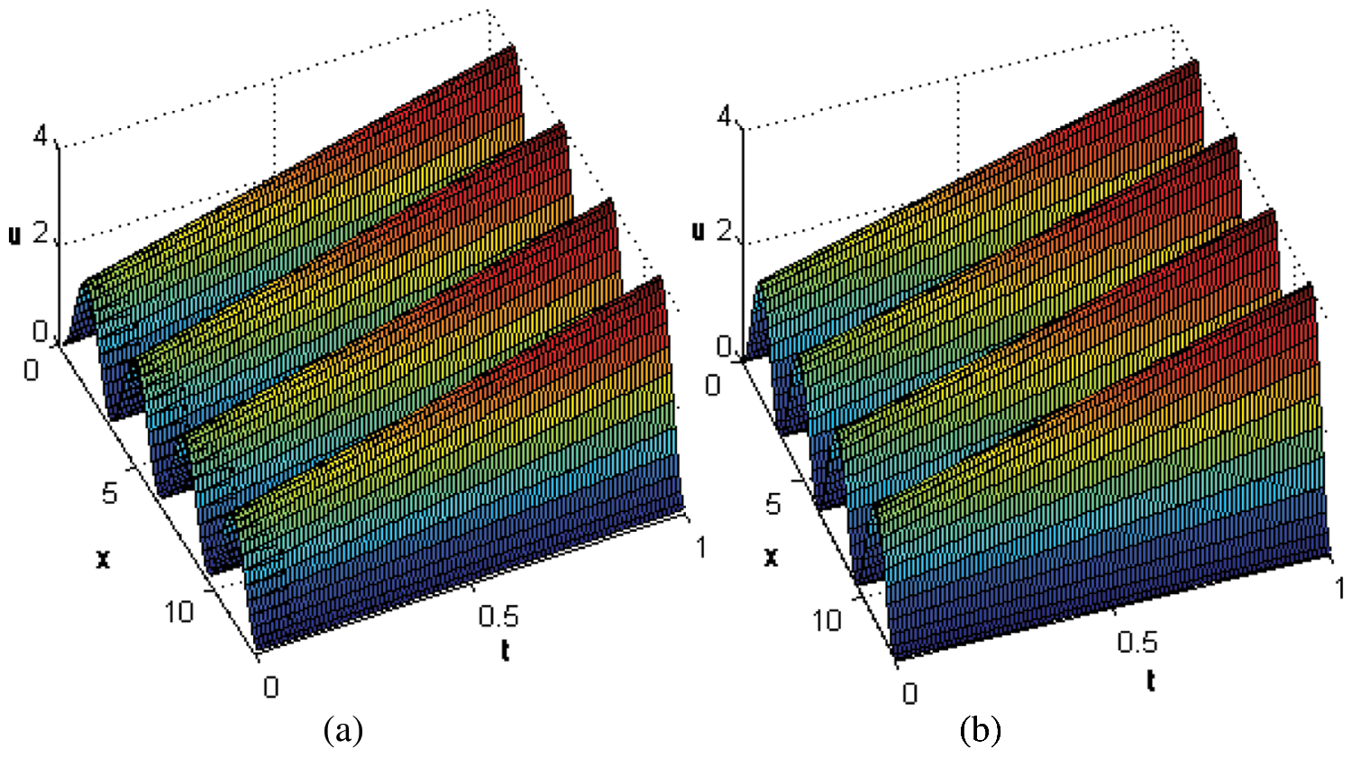
Figure 3: Numerical solutions obtained by (a) CTBS-DQ (b) CTBS-CT, over the time interval [0, 1] using N = 50, , c = 0.1, d = 0.1,

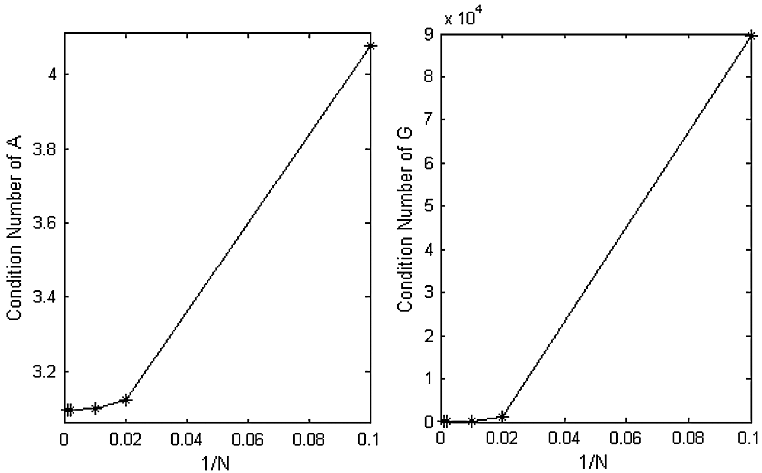
Figure 4: Condition numbers of system matrix A and interpolation matrix G corresponding to the methods (12) and (18) respectively, vs. the number of grid points N, for , c = 0.1, d = 0.1,

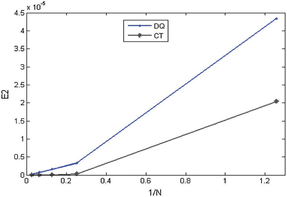
Figure 5: Convergence of the approximate solution in space using , c = 0.1, d = 0.1,

4.2 Problem 2

We take the Eqs. (1)–(3) with the convection-diffusion coefficients c = 0.5, d = 0.005, and . is chosen so that the exact solution of (1)–(3) is given by [8]

The conditions g, g1, g2 are found from Eq. (22). The error norms for different values of and M are computed which are reported in Tabs. 8, 9 alongwith the results of CBSC method [8]. It can be noted from Tab. 8 that errors produced by both the proposed methods decrease as number of nodes N increases. Also both the methods provide considerably better accuracy than the method [8]. Fig. 6 represents solutions obtained using CTBS-DQ and CTBS-CT at M = 1000. Fig. 7 depicts the solution at different time levels.

Table 8: Error norms using M = 100,

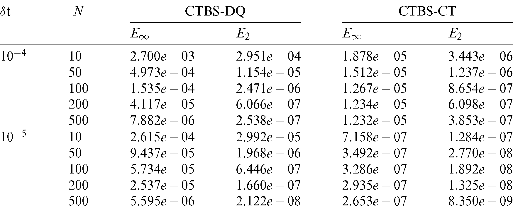
Table 9: Comparison of error norms with CBSC method [8] for N = 100, P = 1

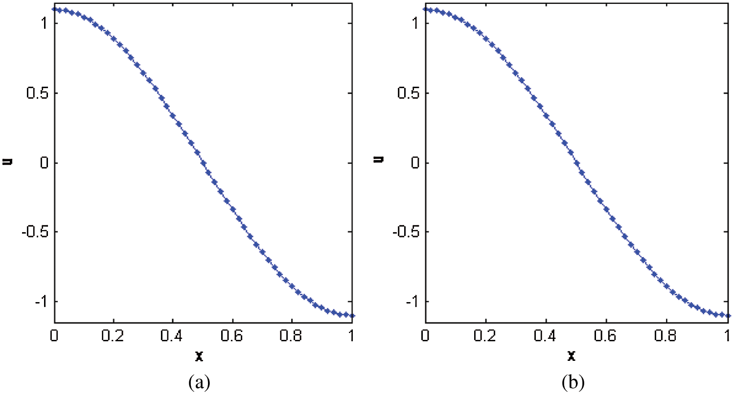
Figure 6: Numerical solutions obtained by (a) CTBS-DQ (b) CTBS-CT, using N = 50, , M = 1000, c = 0.5, d = 0.005,

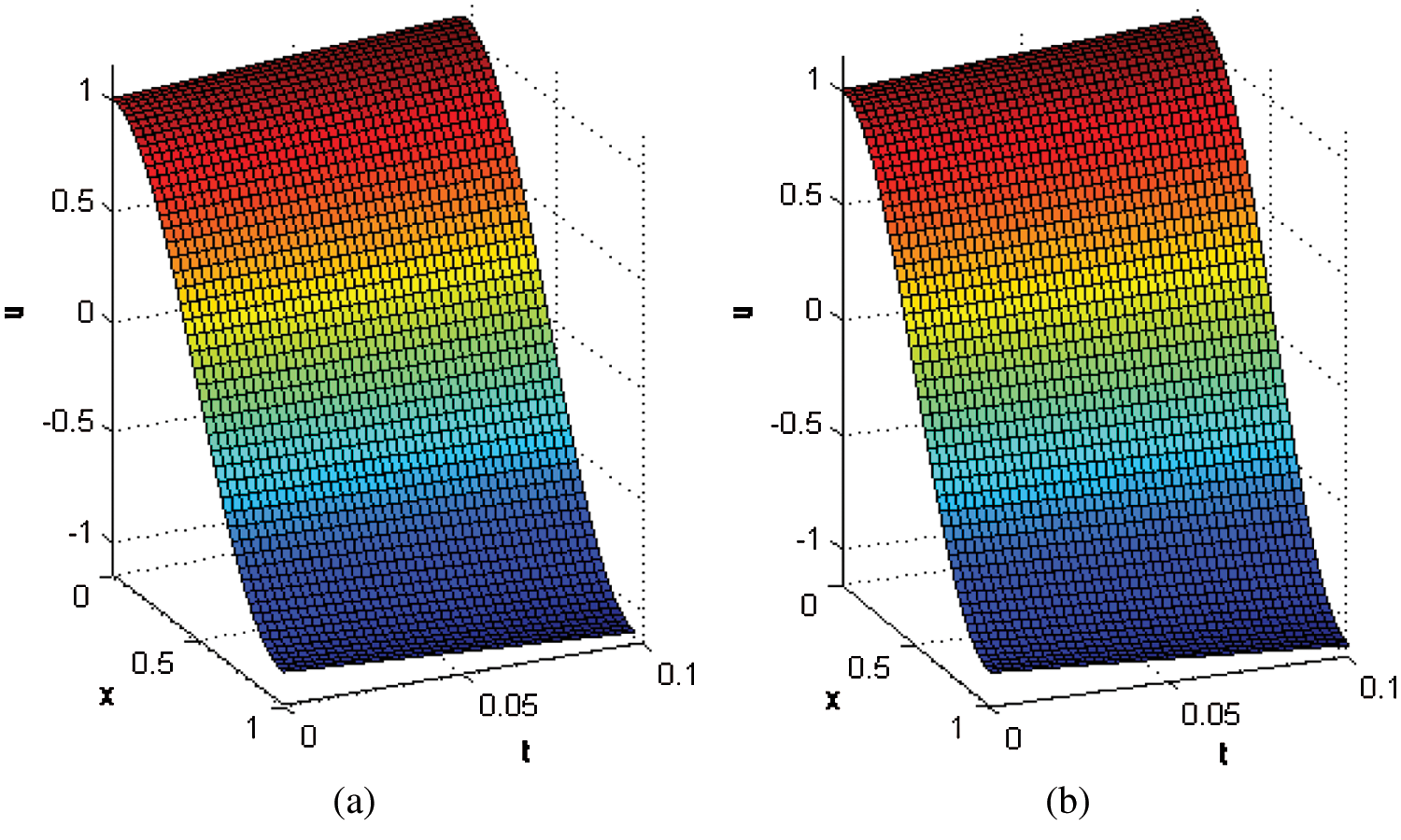
Figure 7: Numerical solutions obtained by (a) CTBS-DQ (b) CTBS-CT, over time interval [0, 0.1] using N = 50, , c = 0.5, d = 0.005,

4.3 Problem 3

For this example we take the convection-diffusion coefficients c = 0.5, d = 0.001 and for the problem (1)–(3) and is chosen so that the exact solution is given by [8]

The conditions g, g1, g2 are found from Eq. (23). The error norms for different values of and M are computed which are provided in Tabs. 10 and 11. It can be noted from Tabs. 10 and 11 that CTBS-CT provided better results than CTBS-DQ. The results in Tab. 11 correspond to convection dominated problem for P = 5. Moreover, the results of the present methods are also compared with the method CBSC [8]. Fig. 8 shows solutions obtained using CTBS-CT at , 0.1. Fig. 9 shows the solution obtained by CTBS-DQ at various time levels.

Table 10: Error norms using M = 100

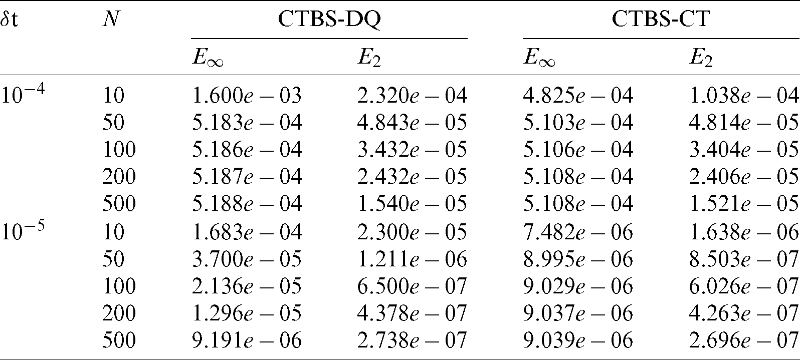
Table 11: Comparison of error norms with CBSC method [8] using N = 100, , P = 5

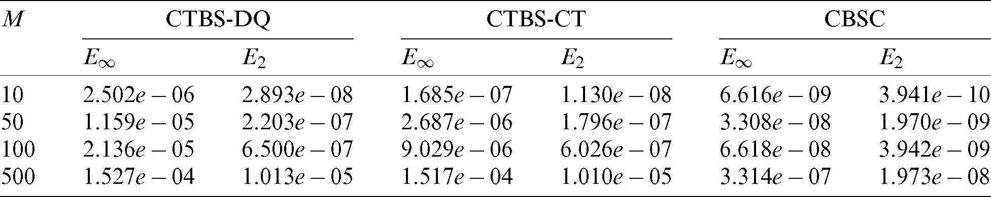
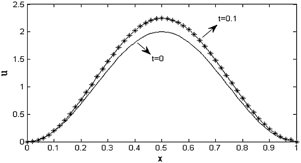
Figure 8: Numerical solutions obtained by CTBS-CT, using N = 50, , c = 0.5, d = 0.001, at t = 0, 0.1

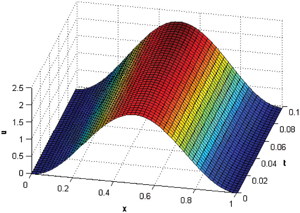
Figure 9: Numerical solutions obtained by CTBS-DQ at different times in the interval [0, 0.1] using N = 50, , c = 0.5, d = 0.001,

5  Conclusion

Two cubic trigonometric B-spline functions based methods are constructed for comparative study of approximate solution of a parabolic type partial integro-differential equation with a weakly singular kernel. The methods are validated using three test problems and the results are compared via error norms. The methods are computationally efficient and improved accuracy is obtained for relatively larger number of spatial nodes. Stability of the methods is shown via spectral radius. It is also observed that condition numbers of the system matrix obtained from cubic trigonometric B-spline collocation method does not increase with increase in the number of spatial nodes and hence the computation remained stable. Both methods do not require much smaller time step to attain high accuracy. In most cases, it is found that cubic trigonometric B-spline collocation method provides better accuracy as compared to cubic trigonometric B-spline differential quadrature. Also, in two examples the cubic trigonometric B-spline collocation technique provided better accuracy than cubic B-spline collocation method. Both techniques have the ability to solve convection dominated and diffusion dominated problems. Due to excellent agreement of these methods with the exact solution, the proposed techniques are efficient in employing to get approximate solution of PIDEs.

Acknowledgement: The authors are thankful to the reviewers for their helpful comments which improved the work of this paper.

Funding Statement: The author(s) received no specific funding for this study.

Conflicts of Interest: The authors declare that they have no conflicts of interest to report regarding the present study.

References

 1.  Gurtin, M. E., Pipkin, A. C. (1968). A general theory of heat conduction with finite wave speeds. Archive for Rational Mechanics and Analysis, 31(2), 113–126. DOI 10.1007/BF00281373. [Google Scholar] [CrossRef]

 2.  Pao, C. V., Payne, L., Amann, H. (2007). Bifurcation analysis of a nonlinear diffusion system in reactor dynamics. Applicable Analysis, 9(2), 107–119. DOI 10.1080/00036817908839258. [Google Scholar] [CrossRef]

 3.  Zadeh, K. S. (2011). An integro-partial differential equation for modeling biofluids flow in fractured biomaterials. Journal of Theoretical Biology, 273(1), 72–79. DOI 10.1016/j.jtbi.2010.12.039. [Google Scholar] [CrossRef]

 4.  Hepperger, P. (2012). Hedging electricity swaptions using partial integro-differential equations. Stochastic Processes and their Applications, 122(2), 600–622. DOI 10.1016/j.spa.2011.09.005. [Google Scholar] [CrossRef]

 5.  Lee, Y. (2014). Financial options pricing with regime-switching jump-diffusions. Computers & Mathematics with Applications, 68(3), 392–404. DOI 10.1016/j.camwa.2014.06.015. [Google Scholar] [CrossRef]

 6.  Larsson, S., Racheva, M., Saedpanah, F. (2015). Discontinuous Galerkin method for an integro-differential equation modeling dynamic fractional order viscoelasticity. Computer Methods in Applied Mechanics and Engineering, 283, 196–209. DOI 10.1016/j.cma.2014.09.018. [Google Scholar] [CrossRef]

 7.  Mirzaee, F., Alipour, S. (2020). A hybrid approach of nonlinear partial mixed integro-differential equations of fractional order. Iranian Journal of Science and Technology, Transactions A: Science, 44(3), 725–737. DOI 10.1007/s40995-020-00859-7. [Google Scholar] [CrossRef]

 8.  Siddiqi, S. S., Arshed, S. (2013). Numerical solution of convection-diffusion integro-differential equations with a weakly singular kernel. Journal of Basic and Applied Science Research, 3(11), 106–120. [Google Scholar]

 9.  Ali, A., Ahmad, S., Shah, S. I. A., Haq, F. (2015). A quartic B-spline colocation technique for the solution of partial integro-differential equations with a weakly singular kernel. Science International, 27(4), 2953–2958. [Google Scholar]

10. Fahim, A., Araghi, M. A. F. (2018). Numerical solution of convection-diffusion equations with memory term based on sinc method. Computational Methods for Differential Equations, 6(3), 380–395. [Google Scholar]

11. Al-Humedi, H. O., Jameel, Z. A. (2020). Combining cubic B-spline Galerkin method with quadratic weight function for solving partial integro-differential equations. Journal of Al-Qadisiyah for Computer Science and Mathematics, 12, 9–20. [Google Scholar]

12. Zhao, Y., Zhao, F. (2016). The analytical solution of parabolic volterra integro-differential equations in the infinite domain. Entropy, 18(10), 344. DOI 10.3390/e18100344. [Google Scholar] [CrossRef]

13. Lopez–Marcos, J. C. (1990). A difference scheme for a nonlinear partial integro-differential equation. SIAM Journal on Numerical Analysis, 27(1), 20–31. DOI 10.1137/0727002. [Google Scholar] [CrossRef]

14. Qiao, L., Xu, D., Wang, Z. (2019). An ADI difference scheme based on fractional trapezoidal rule for fractional integro-differential equation with a weakly singular kernel. Applied Mathematics and Computation, 354, 103–114. DOI 10.1016/j.amc.2019.02.022. [Google Scholar] [CrossRef]

15. Chen, C., Thomee, V., Wahlbin, L. B. (1992). Finite element approximation of a parabolic integro-differential equation with a weakly singular kernel. Mathematics of Computation, 58(198), 587–602. DOI 10.1090/S0025-5718-1992-1122059-2. [Google Scholar] [CrossRef]

16. Avazzadeh, Z., Rizi, Z. B., Ghaini, F. M. M., Loghmani, G. B. (2012). A numerical solution of nonlinear parabolic-type Volterra partial integro-differential equations using radial basis functions. Engineering Analysis with Boundary Elements, 36(5), 881–893. DOI 10.1016/j.enganabound.2011.09.013. [Google Scholar] [CrossRef]

17. Fakhar–Izadi, F., Dehghan, M. (2011). The spectral methods for parabolic Volterra integro-differential equations. Journal of Computational and Applied Mathematics, 235(14), 4032–4046. DOI 10.1016/j.cam.2011.02.030. [Google Scholar] [CrossRef]

18. Long, W., Xu, D., Zeng, X. (2012). Quasi wavelet based numerical method for a class of partial integro-differential equation. Applied Mathematics and Computation, 218(24), 11842–11850. DOI 10.1016/j.amc.2012.04.090. [Google Scholar] [CrossRef]

19. Ali, A., Khan, K., Haq, F., Shah, S. I. A. (2019). A computational modeling based on trigonometric cubic B-spline functions for the approximate solution of a second order partial integro-differential equation. New Knowledge in Information Systems and Technologies, vol. 930, AISC, Spain: Springer Nature Switzerland. [Google Scholar]

20. Mirzaee, F., Alipour, S. (2019). An efficient cubic B-spline and bicubic B-spline collocation method for numerical solutions of multidimensional nonlinear stochastic quadratic integral equations. Mathematical Methods in the Applied Sciences, 43(1), 384–397. DOI 10.1002/mma.5890. [Google Scholar] [CrossRef]

21. Qiao, L., Wang, Z., Xu, D. (2020). An alternating direction implicit orthogonal spline collocation method for the two dimensional multi-term time fractional integro-differential equation. Applied Numerical Mathematics, 151, 199–212. DOI 10.1016/j.apnum.2020.01.003. [Google Scholar] [CrossRef]

22. Abbas, M., Majid, A. A., Ismail, A. I. M., Rashid, A. (2014). The application of cubic trigonometric B-spline to the numerical solution of the hyperbolic problems. Applied Mathematics and Computation, 239, 74–88. DOI 10.1016/j.amc.2014.04.031. [Google Scholar] [CrossRef]

23. Irk, D., Keskin, P. (2016). Cubic trigonometric B-spline Galerkin methods for the regularized long wave equation. Journal of Physics: Conference Series, 766, 12032. DOI 10.1088/1742-6596/766/1/012032. [Google Scholar] [CrossRef]

24. Dag, I., Hepson, O. E., Kacmaz, O. (2017). The trigonometric cubic B-spline algorithm for Burgers’ equation. International Journal of Nonlinear Science, 24(2), 120–128. [Google Scholar]

25. Hashmi, M. S., Awais, M., Waheed, A., Ali, Q. (2017). Numerical treatment of Hunter Saxton equation using cubic trigonometric B-spline collocation method. AIP Advances, 7(9), 95124. DOI 10.1063/1.4996740. [Google Scholar] [CrossRef]

26. Yaseen, M., Abbas, M., Nazir, T., Baleanu, D. (2017). A finite difference scheme based on cubic trigonometric B-splines for a time fractional diffusion-wave equation. Advances in Difference Equations, 2017(1), 291. DOI 10.1186/s13662-017-1330-z. [Google Scholar] [CrossRef]

27. Korkmaz, A., Akmaz, H. K. (2018). Numerical solution of non-conservative linear transport problems. Journal of Applied and Engineering Mathematics, 8(1a), 167–177. [Google Scholar]

28. Tamsir, M., Dhiman, N., Srivastava, V. K. (2018). Cubic trigonometric B-spline differential quadrature method for numerical treatment of Fisher’s reaction-diffusion equations. Alexandria Engineering Journal, 57(3), 2019–2026. DOI 10.1016/j.aej.2017.05.007. [Google Scholar] [CrossRef]

29. Schoenberg, I. J. (1964). On trigonometric spline interpolation. Journal of Mathematics and Mechanics, 13, 795–825. [Google Scholar]

30. Koch, P. E., Lyche, T., Neamtu, M., Schumaker, L. L. (1995). Control curves and knot insertion for trigonometric splines. Advances in Computational Mathematics, 3(4), 405–424. DOI 10.1007/BF03028369. [Google Scholar] [CrossRef]

31. Walz, G. (1997). Identities for trigonometric B-splines with an application to curve design. BIT Numerical Mathematics, 37(1), 189–201. DOI 10.1007/BF02510180. [Google Scholar] [CrossRef]

32. Lyche, T., Winther, R. (1979). A stable recurrence relation for trigonometric B-splines. Journal of Approximation Theory, 25(3), 266–279. DOI 10.1016/0021-9045(79)90017-0. [Google Scholar] [CrossRef]

33. Hamid, N. N. A., Majid, A. A., Ismail, A. I. M. (2010). Cubic trigonometric B-spline applied to linear two-point boundary value problems of order two. World Academy of Science, Engineering and Technology International Journal of Mathematical and Computational Sciences, 4(10), 1377–1382. [Google Scholar]

34. Siraj-ul-Islam Ali, A., Zafar, A., Hussain, A. (2020). A differential quadrature based approach for Volterra partial integro-differential equation with a weakly singular kernel. Computer Modeling in Engineering & Sciences, 124(3), 915–935. DOI 10.32604/cmes.2020.011218. [Google Scholar] [CrossRef]

35. Abbas, M., Majid, A. A., Ismail, A. I. M., Rashid, A. (2014). Numerical method using cubic trigonometric B-spline technique for nonclassical diffusion problems. Abstract and Applied Analysis, 2014(1–6), 1–11. DOI 10.1155/2014/849682. [Google Scholar] [CrossRef]

36. Nazir, T., Abbas, M., Yaseen, M. (2017). Numerical solution of second-order hyperbolic telegraph equation via new cubic trigonometric B-splines approach. Cogent Mathematics, 4(1), 1382061. DOI 10.1080/23311835.2017.1382061. [Google Scholar] [CrossRef]

37. Hepson, O. E., Dag, I. (2017). The numerical approach to the Fisher’s equation via trigonometric cubic B-spline collocation method. Communications in Numerical Analysis, 2017(2), 91–100. DOI 10.5899/2017/cna-00293. [Google Scholar] [CrossRef]

38. Kumar Singh, B., Kumar, P. (2018). An algorithm based on DQM with modified trigonometric cubic B-splines for solving coupled viscous Burgers’ equations. Communications in Numerical Analysis, 2018(1), 21–41. DOI 10.5899/2018/cna-00333. [Google Scholar] [CrossRef]

39. Frazer, R. A., Jones, W. P., Skan, S. W. (1937). ARC R and M 1799. New York: Springer-Verlag New York Inc. [Google Scholar]

40. Zhang, X., Liu, X. H., Song, K. Z., Lu, M. W. (2001). Least-squares collocation meshless method. International Journal for Numerical Methods in Engineering, 51(9), 1089–1100. DOI 10.1002/nme.200. [Google Scholar] [CrossRef]

41. Hsiao, G. C., Kopp, P., Wendland, W. L. (1980). A Galerkin collocation method for some integral equations of the first kind. Computing, 25(2), 89–130. DOI 10.1007/BF02259638. [Google Scholar] [CrossRef]

42. Quan, J. R., Chang, C. T. (1989). New insights in solving distributed system equations by the quadrature method I. Analysis. Computers and Chemical Engineering, 13(7), 779–788. DOI 10.1016/0098-1354(89)85051-3. [Google Scholar] [CrossRef]

43. Bert, C. W., Malik, M. (1996). Differential quadrature method in computational mechanics: A review. Applied Mechanics Reviews, 49(1), 1–28. DOI 10.1115/1.3101882. [Google Scholar] [CrossRef]

44. Bellman, R. E., Casti, J. (1971). Differential quadrature and long-term integration. Journal of Mathematical Analysis and Applications, 34(2), 235–238. DOI 10.1016/0022-247X(71)90110-7. [Google Scholar] [CrossRef]

45. Bellman, R. E., Kashef, B. G., Casti, J. (1972). Differential quadrature: A technique for the rapid solution of nonlinear partial differential equations. Journal of Computational Physics, 10(1), 40–52. DOI 10.1016/0021-9991(72)90089-7. [Google Scholar] [CrossRef]

46. Shu, C. (2000). Differential quadrature and its application in engineering. London: Springer-Verlag. [Google Scholar]

47. Ahmad, I., Ahsan, M., Hussain, I., Kumam, P., Kumam, W. (2019). Numerical simulation of PDEs by local meshless differential quadrature collocation method. Symmetry, 11(3), 394. DOI 10.3390/sym11030394. [Google Scholar] [CrossRef]

48. Khan, M. N., Siraj-ul-Islam, Hussain, I., Ahmad, I., Ahmad, H. (2020). A local meshless method for the numerical solution of space-dependent inverse heat problems. Mathematical Methods in the Applied Sciences, 2020, 1–14. [Google Scholar]

49. Bashan, A. (2019). An efficient approximation to numerical solutions for the Kawahara equation via modified cubic B-spline differential quadrature method. Mediterranean Journal of Mathematics, 16(1), 708717. DOI 10.1007/s00009-018-1291-9. [Google Scholar] [CrossRef]

50. Korkmaz, A., Dag, I. (2011). Shock wave simulations using Sinc differential quadrature method. Engineering Computations, 28(6), 654–674. DOI 10.1108/02644401111154619. [Google Scholar] [CrossRef]

51. Arora, G., Joshi, V. (2018). A computational approach using modified trigonometric cubic B-spline for numerical solution of Burgers’ equation in one and two dimensions. Alexandria Engineering Journal, 57(2), 1087–1098. DOI 10.1016/j.aej.2017.02.017. [Google Scholar] [CrossRef]

52. Ghafoor, A., Haq, S., Hussain, M., Kumam, P., Jan, M. A. (2019). Approximate solutions of time fractional diffusion wave models. Mathematics, 7(10), 923. DOI 10.3390/math7100923. [Google Scholar] [CrossRef]

53. Siraj-ul-Islam, Haq, S., Ali, A. (2009). A meshfree method for the numerical solution of the RLW equation. Journal of Computational and Applied Mathematics, 223(2), 997–1012. DOI 10.1016/j.cam.2008.03.039. [Google Scholar] [CrossRef]

This work is licensed under a Creative Commons Attribution 4.0 International License, which permits unrestricted use, distribution, and reproduction in any medium, provided the original work is properly cited.