Computer Modeling in Engineering & Sciences

DOI: 10.32604/cmes.2021.014284

ARTICLE

Impacts of Disk Rock Sample Geometric Dimensions on Shear Fracture Behavior in a Punch Shear Test

Tantan Zhu*and Yao Li

School of Highway, Chang’an University, Xi’an, 710064, China
*Corresponding Author: Tantan Zhu. Email: tantan.zhu@chd.edu.cn
Received: 15 September 2020; Accepted: 03 December 2020

1  Introduction

Shear fracture is one of the fundamental failure patterns of rocks. At present, Mohr–Coulomb criterion is widely used for the determination of shear strength and the envelope, which intercepts the -axis at cohesion with a slope equal to internal friction angle, is assumed to be a straight line in the plane [1–3]. The internal friction angle and cohesion, which are based on Mohr–Coulomb theory, are important shear mechanical parameters used for rock engineering design [4,5]. These shear mechanical parameters are mainly determined by triaxial compression tests [6–8] or direct shear tests (DST) [9–12].

In a triaxial compression test, the sample fails under axial and confining stresses. The strength envelope can be obtained by the tangent line of the Mohr’s stress circles based on minimum and maximum principal stresses [13,14]. However, the normal and shear stresses on the shear plane cannot be directly obtained from triaxial compression test results. Unlike the triaxial compression test, the DST can directly measure the normal and shear stresses on the shear plane [15,16]. There are two commonly used methods in this category: Direct shear-box test and punch shear test (PST). For the direct shear-box test, upper and lower shear boxes are the main component of the shear device. Samples in the shear-box test are subjected to normal and shears stresses and fails along an approximate plane. However, when the sample is subjected to the PST, it fails along a cylindrical surface rather than a plane (as shown in Fig. 1). Originally, the PST was proposed for conveniently determining the direct shear strength [17]. Shear stress is applied by a compressive force within and parallel to the shear surface during the PST. The PST is applicable for high strength solids, minimizes the bending stress on the samples, and facilitates sample preparation [17,18]. Thus, other testing methods, such as the punch through shear test which uses a rock disk sample with two circular notches, was proposed based on the PST to determine shear mechanical parameters [19–21].

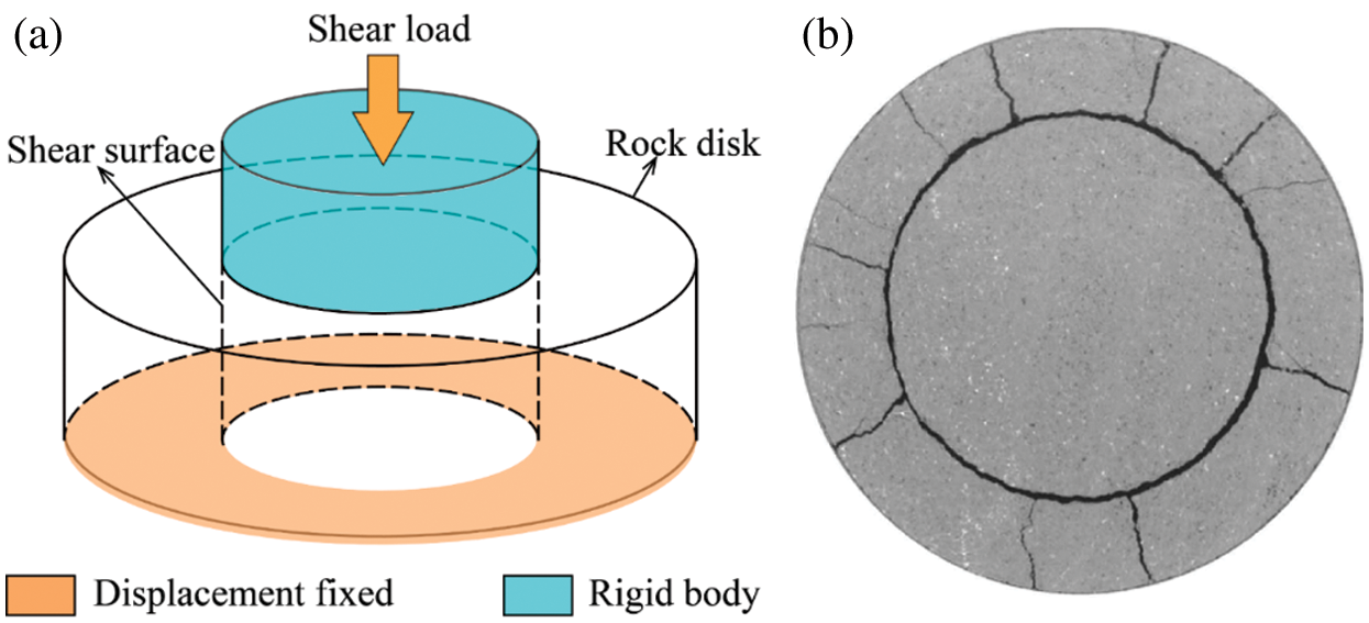
Figure 1: Punch shear test: (a) Schematic diagram; (b) Fracture pattern [22]

Rock sample dimensions in laboratory tests significantly impact the test result. As shown in Fig. 2, the tested sample in the PST has three important geometric dimensions, disk diameter (D), shear surface diameter (Di), and disk height (H), all of which influence the test result. However, unlike the uniaxial and triaxial compression test, which use a cylindrical sample with a height-diameter ratio of two, no standard sample size is specified for the PST. For example, Xu et al. [22] used disk samples with the D = 38 mm, Di = 25.4 mm, and H = 15 mm to carry out a PST for the investigation of dynamic shear response of rocks. Huang et al. [23] also carried out a PST under a dynamic load, but the dimensions of their samples were D = 57 mm, Di = 25 mm, and H = 14 mm. Backers et al. [24] conducted a punch through shear test using disks with the D = 50 mm and Di = 25 mm. As the geometric dimensions of the samples used in these studies are different, the results are not directly comparable. Therefore, the influence of the sample dimensions on shear behavior should be analyzed further and a standard sample dimension should be created for PST.

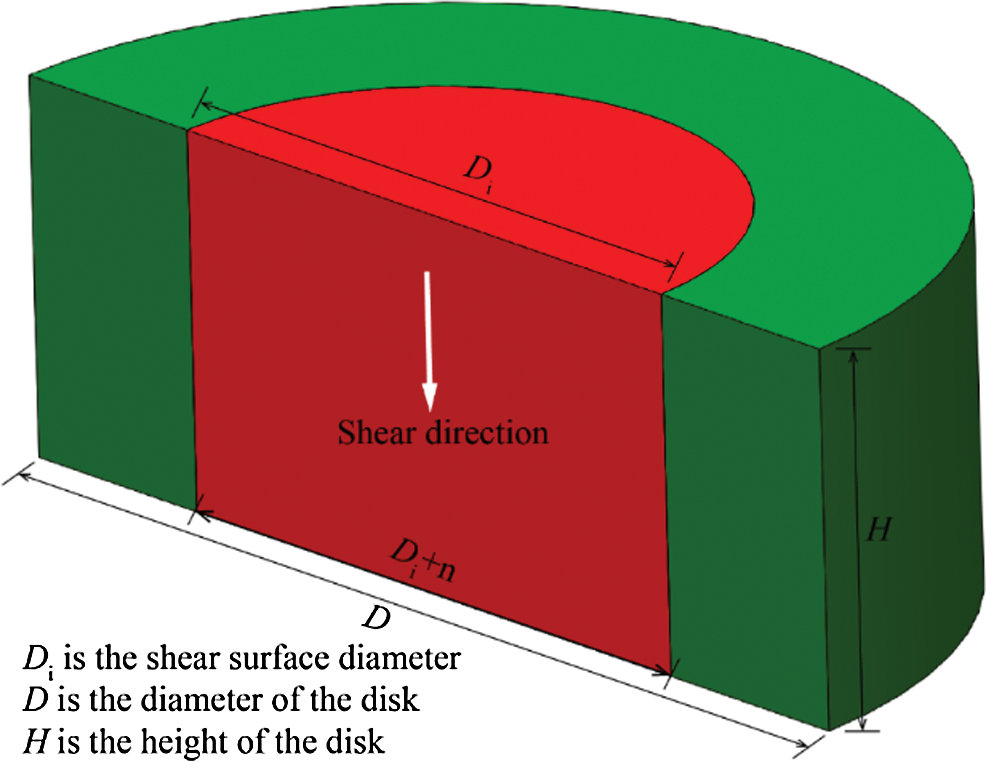
Figure 2: Geometrical dimensions of the disk used for PST (half of the disk)

To investigate the influence of the geometric dimensions of the sample disk on the shear behavior of rocks in the PST, punch shear simulations were carried out under zero normal stress by using Particle Flow Code (PFC). Variations in shear mechanical parameters under various geometries were studied. Then, the failure process and fracture pattern of disks with different disk dimensions were investigated. Finally, the normal stress on the shear surface during the test was analyzed and a suggested disk size was given.

2  Particle Flow Code and Simulation Methodology

2.1 Particle Flow Code

PFC3D, a three-dimensional discrete element modeling framework, has been widely used in rock mechanical simulations. The model framework simplifies rock material into balls and bonds. A ball in the PFC3D is a rigid and the surface of the ball is defined by radius. A ball has a single set of surface properties. Balls can translate and rotate. As linear parallel-bond can transmit both force and moment while contact-bond only transmits force [25–27], it was selected to conduct the PST simulations. For the parallel-bond, the contact force and moment are updated as follows:

where Fc is contact force; Fl and Fd is linear force and dashpot force, respectively; is parallel-bond force; Mc is contact moment; is parallel-bond moment. The parallel-bond contact force consists of a normal force and a shear force , and the parallel-bond moment consists of a twisting moment and a bending moment :

where nc is the direction of the contact plane. The parallel-bond shear force and bending moment line on the contact and are expressed as:

The force–displacement law for the parallel-bond force and moment consists of the following seven steps.

1.    Update the bond cross-sectional properties. In this step, the radius R, cross-sectional area A, moment of inertia I, the polar moment of inertia J of parallel-bond will be calculated:

2.    Update normal force. The normal force will be recalculated according to the relative normal-displacement increment , normal stiffness of the parallel-bond , and the area of the parallel A:

3.    Update shear force. Shear force of the parallel-bond will be recalculated in this step:

where ks is shear stiffness of the parallel-bond and is the relative shear–displacement increment.

4.    Update twisting moment:

where is a relative twist-rotation increment.

5.    Update bending moment:

where is relative bend-rotation increment.

6.    Update the maximum normal and shear stresses at the parallel-bond periphery:

where is moment-contribution factor.

7.    Enforce strength limits. If the tensile strength limit of the parallel-bond is exceeded, then break the bond in tension. If the shear strength limit of the parallel-bond is exceeded, then break the bond in shear.

2.2 Simulation Methodology

In PFC3D, stress is applied within the model by moving walls or balls. If the tensile or shear strength of a bond is exceeded, a tensile or shear micro-crack will be formed. The numerical model in this study is composed of five walls (Fig. 3a). The diameter of the first wall (Wall #1), a circular wall, is equal to the Di. The second wall (Wall #2) is in the shape of a ring and has an outer diameter larger than the D and an inner diameter smaller than the Di. The diameter of the third wall (Wall #3) is larger than Di + n. The inner diameter of the fourth wall (Wall #4) is equal to the Di of the sample plus an additional four millimeters, and with an outer diameter larger than the D The fifth wall (Wall #5) is a cylindrical wall with a diameter equal to the D. These five walls ensure that the simulated rock material does not leave the domain (Fig. 3b). Once the simulated rock material was bonded by contacts (Fig. 3c), Wall #2 and #3 were removed from the model domain before finalizing the numerical model and applying displacement and stress. According to Xu et al. [22] and Huang et al. [23], the shear surface is not a standard cylinder, with the bottom diameter of the shear cylinder slightly larger than the top diameter. Shear stress on the shear surface can be calculated by dividing the shear force by the area of the shear surface. In the PST, the average diameter of the shear surface is (2Di + n)/2. Thus, the shear stress on the shear surface can be calculated as:

where P is the shear load and n are the difference between the top diameter and bottom diameter of the shear surface.

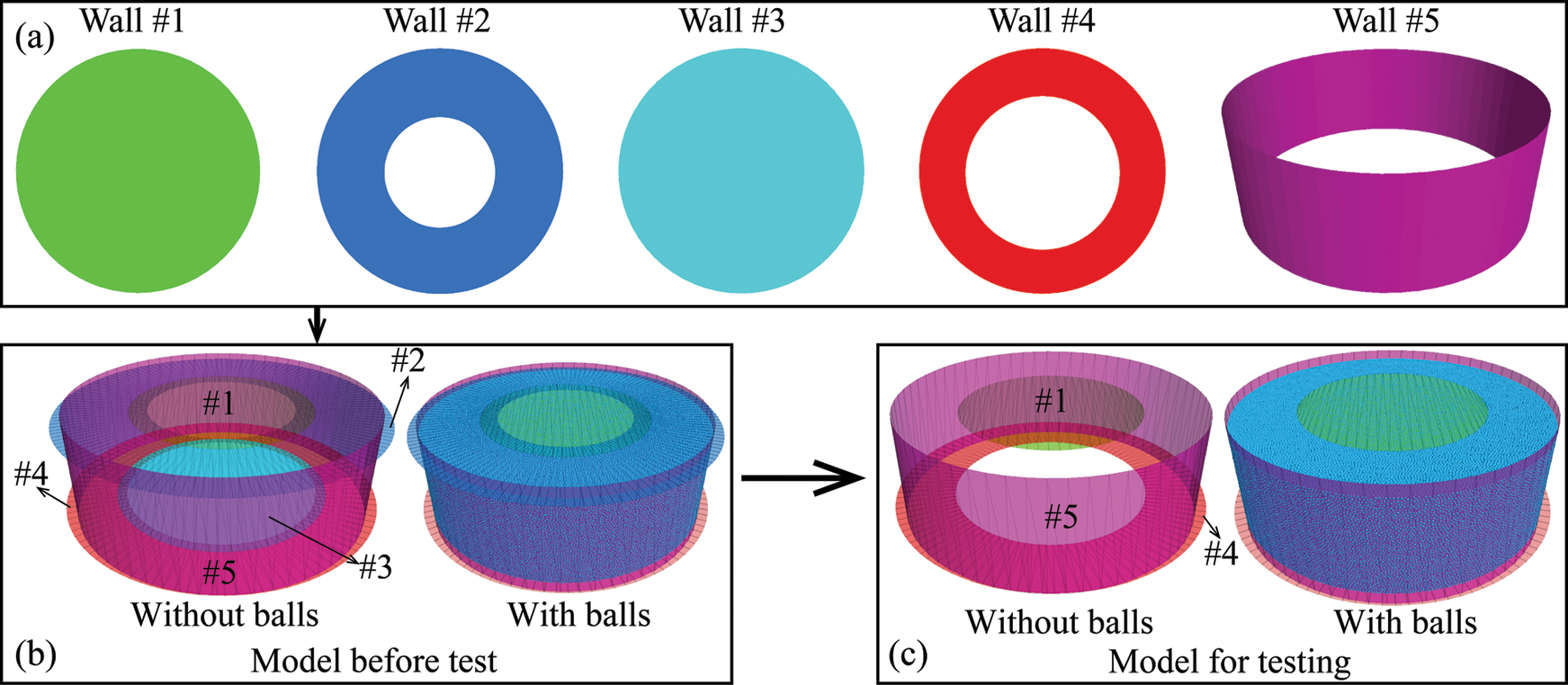
Figure 3: Numerical model of the disk used for simulation (a) shows the shapes of the walls; (b) is the numerical sample with all the walls; (c) is the numerical sample with the walls #2 and #3 deleted

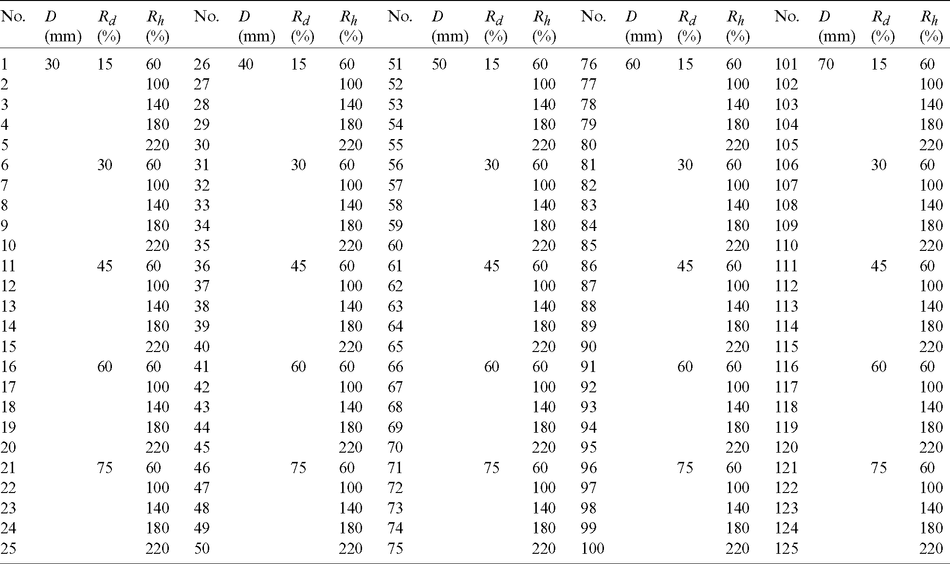
As the strength of a parallel-bond conforms to the Mohr–Coulomb criterion. Therefore, the strength of a parallel-bond can be described by the parameters of parallel-bond tensile strength, parallel-bond cohesion and parallel-bond friction angle. The detailed descriptions of the micro-parameters used in the simulations are detailed in Tab. 1. During the test, Wall #4 was fixed and shear stress was applied by the vertical movement of the Wall #1. A displacement rate of 0.08 m/s was adopted for shear stress loading, which is low enough for a static rock loading simulation [2,28]. As this study aimed to investigate the influence of geometric dimensions of a rock disk on shear behavior and provide a recommended sample size for the PST, the confining stress applied by Wall #5 was set to zero. The PST simulations were conducted on disks with a D from 30 to 70 mm at intervals of 10 mm. The ratio between Di and D (Rd) ranged from 0.15 to 0.75 in intervals of 0.15. The ratio between H and Di (Rh) varied from 0.6 to 2.2 with an interval of 0.4. In addition, the bottom diameter of the surface was also defined as 4 mm larger than the applied Di (i.e., n = 4 mm in Eq. (15)). Tab. 2 provides detailed descriptions of the geometric dimensions of the 125 samples used in the numerical simulations.

Table 1: Micro-parameters used for PST simulation

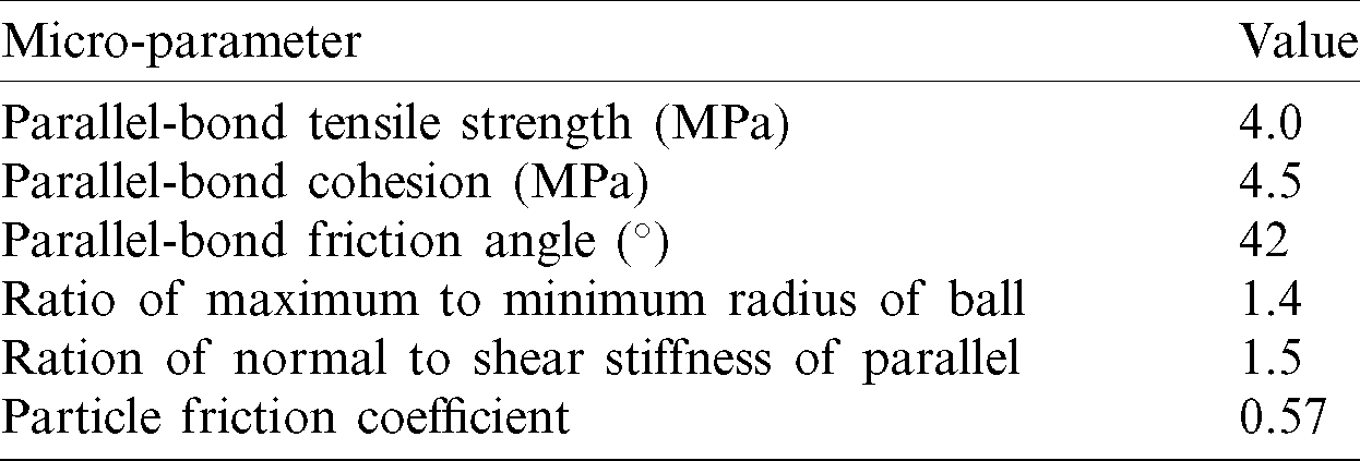
Table 2: Detailed description for geometrical dimensions of the disks used for PST simulation

3  Results and Analysis

3.1 Strength and Deformation

Twenty-five of the 125 samples were selected for analysis. Figs. 4a–4c give the curves with various D (Rd = 0.45, Rh = 0.6), Rd (D = 50 mm, Rh = 0.6), and Rh (D = 50 mm, Rd = 0.45), respectively. The shear stress–shear displacement curves can be divided into three stages: linear, nonlinear, and post-peak (Fig. 4). In the linear stage, shear stress exhibits linear growth as shear displacement increases. As the shear stress–shear displacement curve enters a nonlinear stage, shear stress increases nonlinearly with increased shear displacement. In the post-peak stage, the shear stress decreases gradually as the shear displacement increases. The shear stress of the samples with a higher Rh decreases more slowly, which is even more obvious in Fig. 4c. Between the linear and nonlinear stages, most of the samples have a distinct drop in shear stress, except for the sample with the D = 50, Rd = 0.75, Rh = 0.6, the sample with the D = 50, Rd = 0.45, Rh = 1.8, and the sample with the D = 50, Rd = 0.45, Rh = 2.2 (Figs. 4b, 4c). Shear strength and shear stiffness of samples with varying geometric dimensions differ, indicating that geometric dimensions of the sample disk have significant effects on the behavior of shear mechanics.

Figure 4: Shear stress–shear displacement curves of samples with (a) Rd = 0.45 and Rh = 0.6, (b) D = 50 mm Rh = 0.6, (c) D = 50 mm and Rd = 0.45

Fig. 5 shows the influence of disk geometric dimensions on the shear strength in the PST. When the Rd is equal to 0.15, the shear strength increases and then stays at a high level with the increase of the Rh except for the sample with the D equal to 30 mm, which shows a constant increase (Fig. 5a). For all of the samples with the Rd equal to 0.3, the shear strength initially grows and then declines. However, the shear strength of the samples with the Rd equal to 0.45 first increases and then decreases when the D is 30 and 40 mm (Figs. 5a and 5b), which reduces gradually when the D is in the range from 50 to 70 mm (Figs. 5c–5e). When the Rd is equal to 0.6 or 0.75, shear strength of all samples reduces gradually as the Rh grows. Shear strength gradually decreases as the Rd increases from 0.3 to 0.75 (Fig. 5). As shown in Fig. 5f, the shear strength gradually approaches a constant as the Rd and Rh increase. However, the shear strength of the samples with different D values varies little.

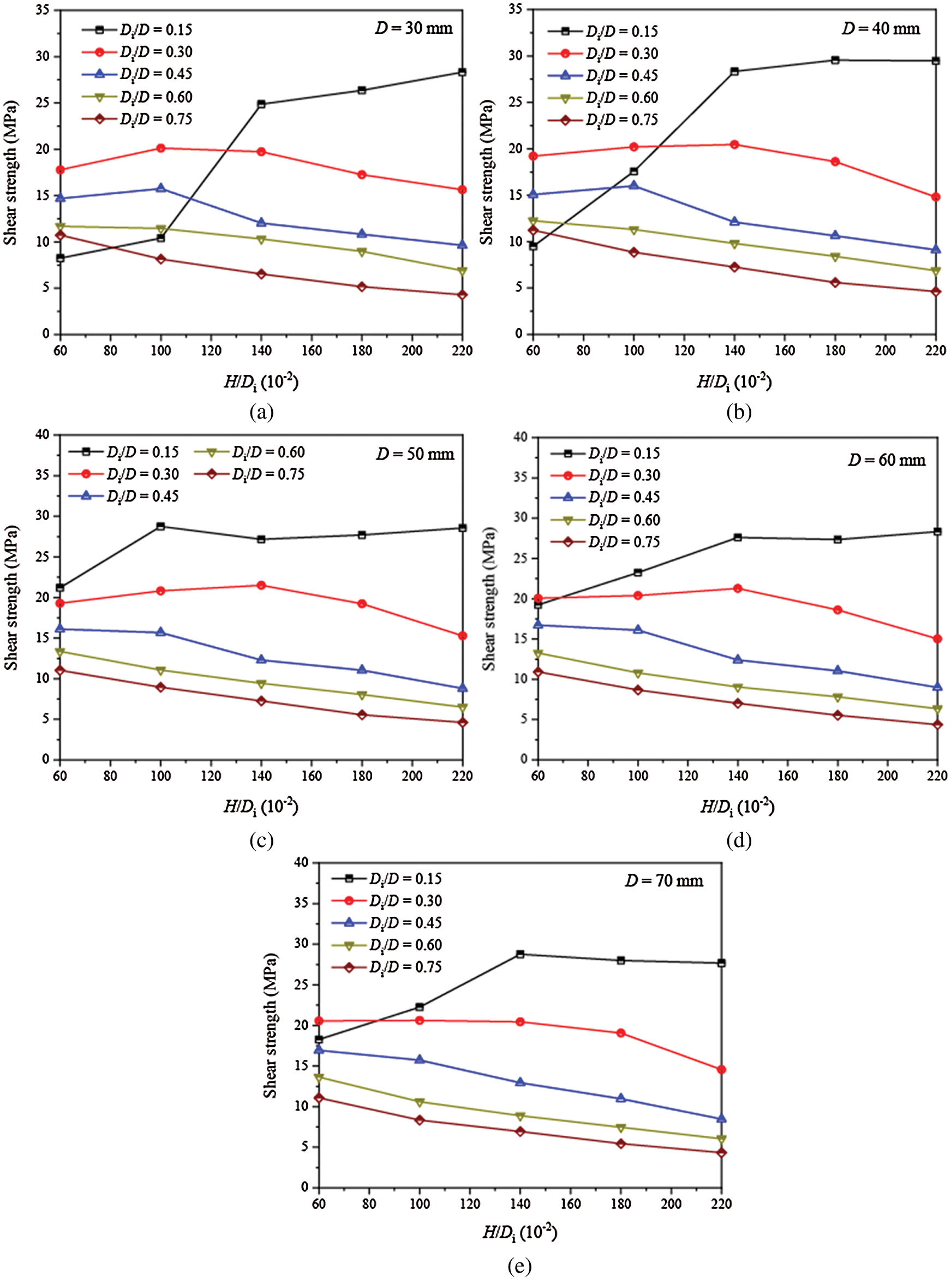
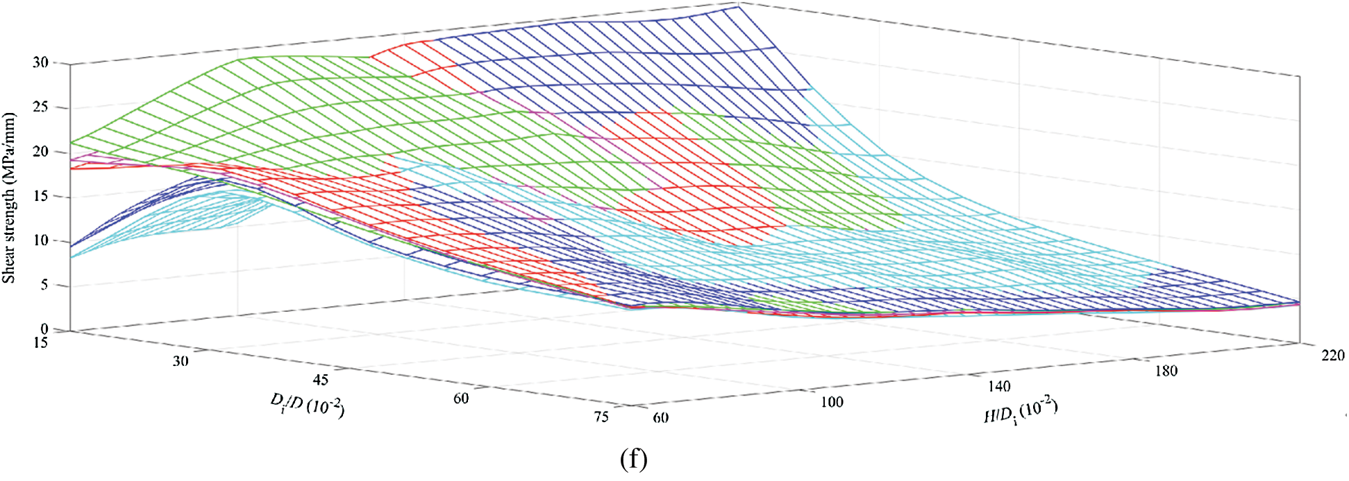
Figure 5: Shear strength of disks with various disk geometrical dimensions (a–e) are the changes in shear strength of samples with different disk diameter and (f) shows the relationship between shear strength, H/Di and Di/D in a three-dimensional coordinate system

In the linear stage, the shear stress increases linearly with the increase of the shear displacement (Fig. 4). The slope of this linear increase is the shear stiffness of the disk in the PST (Fig. 6). The shear stiffness decreases nonlinearly with the growth of the Rd and the Rh (Fig. 6). Additionally, it can be seen that the shear stiffness reduces gradually as the disk diameter D increases (Fig. 6b). The difference of the shear stiffness with various values of D is larger when the sample has a smaller Rd or Rh. As shown in Fig. 6a, for samples with a Rd of 0.15 and a Rh of 0.6, the maximum shear stiffness is 175.21 MPa/mm while the minimum shear stiffness is 114.85 MPa/mm. However, for the samples with a Rd of 0.75 and a Rh of 2.2, the maximum and the minimum shear stiffness are 8.21 and 3.99 MPa/mm, respectively. Thus, the shear stiffness of a sample is more sensitive to the D in the PST when the Rd and Rh is small. With the increase of the Rd and Rh, the shear stiffness gradually approaches a threshold and the difference in shear stiffness between different samples with varying D reduces (Fig. 6b), similar to the results for shear strength (Fig. 5).

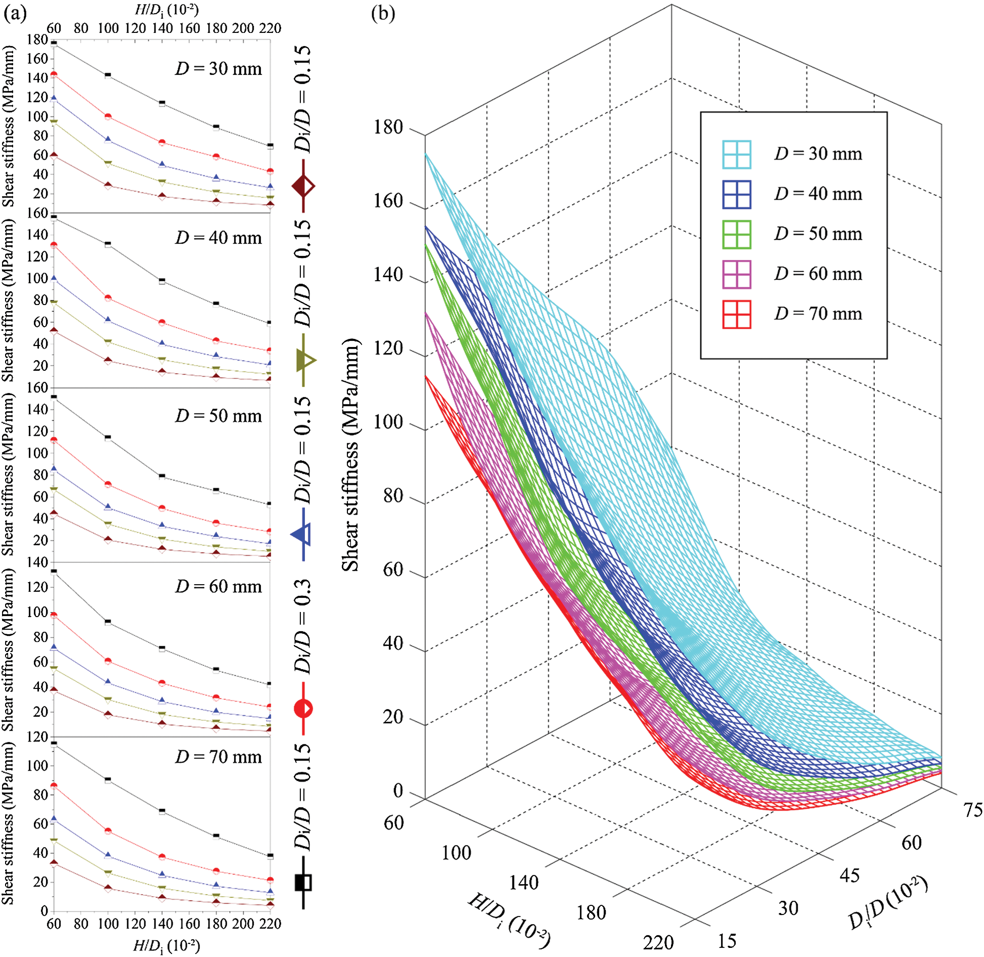
Figure 6: Change in shear stiffness of disks with various geometrical dimensions (a) shows the changes in shear stiffness of samples with different disk diameter and (b) shows the relationship between shear stiffness, H/Di and Di/D in a three-dimensional coordinate system

The change in normal displacement with shear displacement is shown in Fig. 7. The variation of the normal displacement can be divided into three stages: Initial stage, acceleration stage, and linear stage. In the initial stage, the normal displacement increases slowly as the shear displacement increases. It can be observed that the initial stage in Fig. 7 corresponds to the timing of the linear stage in Fig. 4. The acceleration stage is nonlinear, with the normal displacement growth rate increasing gradually. This stage corresponds to the stage near the peak shear stress of the curves in Fig. 4. In this stage, the shear stress–shear displacement changes from pre-peak to post-peak. In the linear stage in Fig. 7, the normal displacement increases linearly with the growth of the shear displacement. This stage corresponds to the post-peak stage in Fig. 4. The slope of the curve in Fig. 7 is the shear dilatancy angle of the sample in the PST. Based on these results, the change in normal displacement with shear displacement can be simplified into the curve shown in Fig. 8. The three types of dilatancy angles are the slopes of the three stages on the curve in Fig. 7. Where the peak dilatancy angle is the slope of the normal displacement-shear displacement curve at peak shear stress.

Figure 7: Normal displacement-shear displacement curves of samples with various (a) D, (b) Di and (c) H

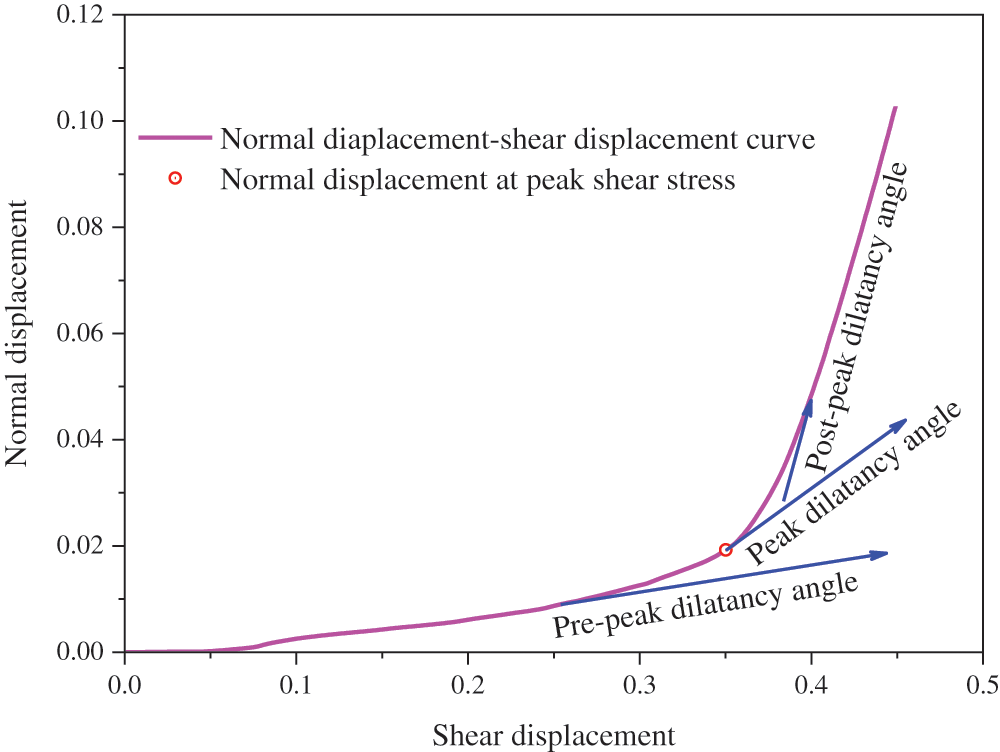
Figure 8: Three types of dilatancy angle

Fig. 9 gives the dilatancy angle of disks in the PST. The abscissa in Fig. 9a is the sample number listed in Tab. 2, in which the detailed geometric dimensions for each sample are presented. An increase in the abscissa means an increase in D, Di, or H (Tab. 2). For the disks with the same D, the pre-peak dilatancy angle first increases and then decreases as the sample number increases in general, and all of the maximum pre-peak dilatancy angles are obtained when both Rd and Rh are equal to 0.6 (i.e., the samples numbered 16, 41, 66, 91 and 116) (Fig. 9a). The pre-peak dilatancy angle exhibits such a change due to the pre-peak dilatancy angle first growing and then reducing with the increase of the Rd under the same Rh (Fig. 9b). Meanwhile, the pre-peak dilatancy angle increases gradually with the increase of the Rh for the samples with a small Rd while that decreases as the Rh grows when the Rd is higher (Fig. 9b). For the samples with different D and the same Rh and Rd, the pre-peak dilatancy angle exhibits little difference. For example, the five maximum pre-peak dilatancy angles mentioned above are 4.58, 4.61, 4.56, 4.40, and 4.43 MPa/mm, respectively, with the difference between the maximum and the minimum value being 0.21 MPa/mm. For each sample, the peak dilatancy angle is smaller than the post-peak dilatancy angle, which can be easily understood through analyzing Fig. 8. With the increase of the sample number, the peak and post-peak dilatancy angles first increase, then remain at a high value, but in general grow slowly. The peak and post-peak dilatancy angles of the samples with a Rd of 0.15 and a Rh equal to 0.6 and 1.0 are very small compared to the other samples. Thus, the variation of the Rd and Rh has little influence on the peak and post-peak dilatancy angles except when the two parameters are small (Rd equal to 0.15 and Rh of 0.6 or 1.0). Similar to the pre-peak dilatancy angle, the peak and post-peak dilatancy angles have little difference for the samples with the same Rd, Rh but different D. Therefore, the influence of the disk diameter D on dilatancy angle is negligible.

Figure 9: Change in dilatancy angles of disks in the PST (a) Shows the changes in the three types of dilatancy angles for the samples with various geometrical dimensions; (b) Shows the relationship between dilatancy angle, H/Di and Di/D in a three-dimensional coordinate system

3.2 Fracture Characteristic

Fig. 10 gives the fracture process of the samples with a D of 50 mm and a Rd equal to 0.3. In the same picture, the circular image on the left is the top view while the rectangular image on the right is the front view of the disk. In the top view, the larger circle is the disk outline and the smaller circle is shear surface. All pictures in the same row show the same sample (Fig. 10, rows A–E). The pictures (the top five columns on the left) in the same column show the fracture pattern of the samples under the same percent (0.2–1.0 with and interval of 0.2) of corresponding peak shear stress . The two columns on the far right show the post-peak fracture patterns of samples and their 3D view. It is worth noting that the front view of the sample is not drawn to scale for the sake of brevity and illustration. The samples have begun to crack when the shear stress reaches 0.2 (Fig. 10, column 1). Some of the cracks are near the shear surface while others appear at the edge of the sample. Cracks near the shear surface are formed due to the increase of the shear displacement and shear stress. As shear stress increases, the number of cracks near the shear surface grows significantly. However, the cracks at the edge of the sample do not expand before the pre-peak stage. At peak shear stress and in the post-peak stage, a large number of micro-cracks have been produced at the shear surface, forming multiple macro-cracks along the radial direction of the samples (Fig. 10, columns 5 and 6). The fracture pattern of the sample is very close to that in the laboratory test shown in Fig. 1b. When the Rh is less than or equal to 1.4, three macro-cracks are formed within the shear surface when the shear stress reaches (Fig. 10, rows A–C, column 3). This kind of macro-crack is also produced in the sample with a Rh of 1.8 when the shear stress reaches (Fig. 10, row D, column 4). Bending of the sample within the shear surface, caused by the load parallel to shear displacement, results in tensile stress on the lower surface of the sample. This is the main cause of the formation of the three macro-cracks. The three macro-cracks are produced only on the lower surface of the samples with a Rh of 1.0, 1.4, and 1.8, while they propagate to the vertical middle of the sample when the Rh is 0.6 due to the thinness of that sample. In addition, micro-cracks propagate from both vertical ends to the middle when the Rh is 0.6 and 1.0 (Fig. 10, rows A and B, column 3) while the micro-cracks propagate from one end to the other end when the Rh is 1.8 and 2.2 (Fig. 10, rows D and E, column 3).

Figure 10: Fracture process of the samples with D = 50 mm and Rd = 0.3. The circular picture is the top view and the rectangular picture is the front view of disks. In the top view, the two circles are the disk outline and the shear surface, respectively. In the front view, the two vertical lines are the boundary of the shear surface

According to Huang et al. [29], shear failure rate Rs is defined as the ratio of shear crack number to total crack number in a rock test simulation. This can be used to describe the fracture pattern. Take the samples with a D of 50 mm and a Rd of 0.6 as examples (Fig. 11). In the initial stage, the Rs fluctuates as the sample has fewer cracks and the formation of a new crack will have a significant impact on the value of Rs. After the initial fluctuations, the Rs is small (less than 0.5) and begins to increase rapidly, indicating that the sample fails due to tension in the beginning. Then, the Rs remains at a high level (greater than 0.5) before peak shear stress, indicating that the fracture of a sample is mainly caused by the formation of shear crack at this stage. In the post-peak stage, the Rs reduces gradually with the increase of the total crack number. This suggests that more tensile cracks rather than shear cracks are formed after peak shear stress.

Figure 11: Change in Rs of the samples with the D = 50 mm and Rd = 0.3 and partial enlarged

Fig. 12 gives the change in peak shear failure rate (Rsp), which is the Rs at peak shear stress. As first introduced in Fig. 9a, the abscissa in Fig. 12a is the sample number listed in Tab. 2. On the whole, the peak shear stress gradually increases with the growth of the sample number (Fig. 12a). For the samples with a Rd of 0.15 and a Rh of either 0.6 or 1.0, the D of the sample has a marked impact on the Rsp. (Fig. 12a, samples 1, 2, 26, and 27) When the Rd is larger than 0.15 or the Rh is greater than 1.0, the Rsp remains high (greater than 0.5) and fluctuates as the sample number increases (Fig. 12b). Thus, samples mainly fail due to shear stress and the Rsp is not sensitive to the D when the Rd is larger than 0.15 or the Rh is greater than 1.0.

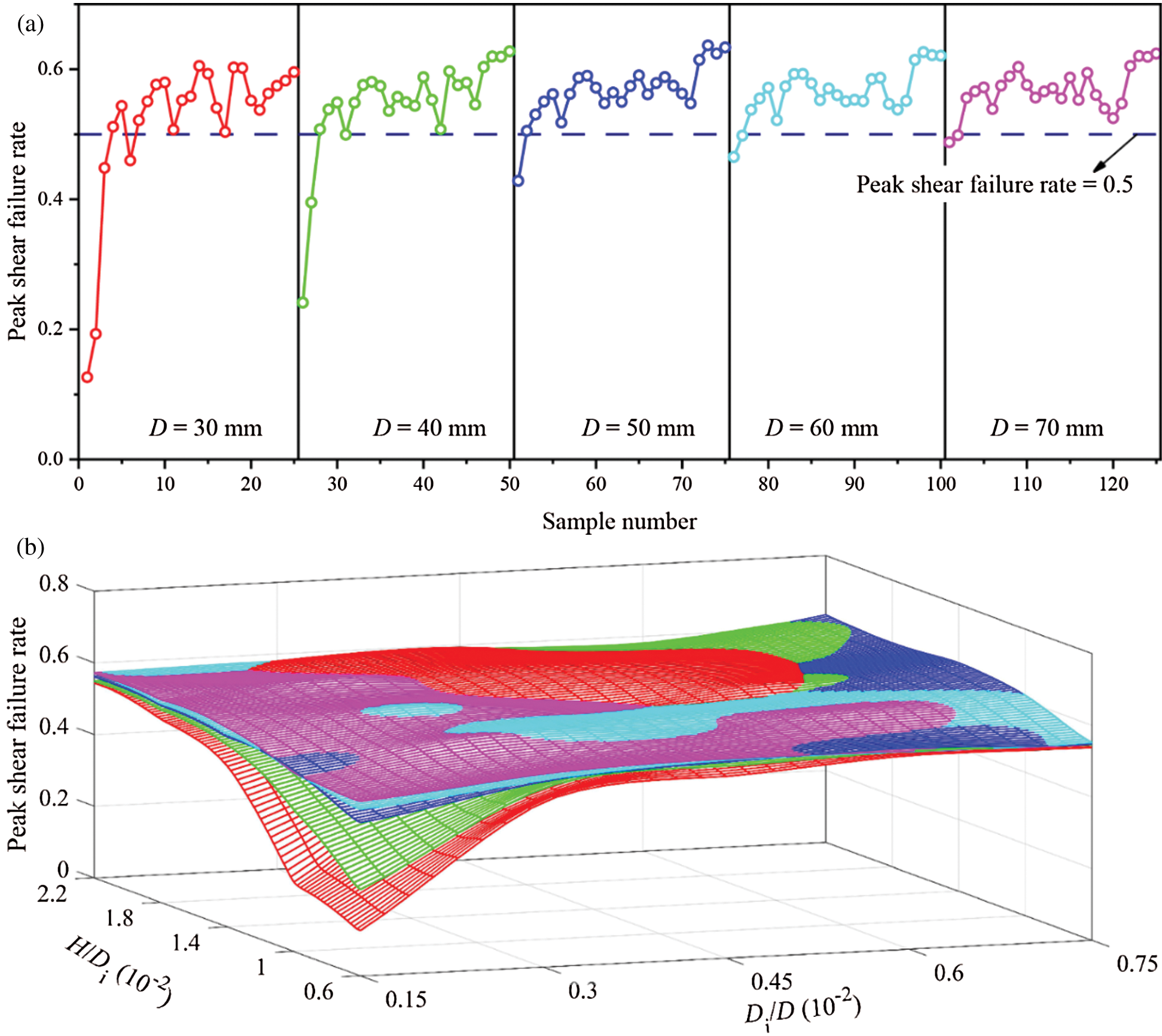
Figure 12: Change in peak shear failure rate. In which, (a) Displays the change of peak shear failure rate in a two-dimensional coordinate system, and (b) Displays the change of that in a three-dimensional coordinate system

As shown in Fig. 13, bonds in the PFC model consist of two ends, with each end connecting with a piece. The angle between the vector along each bond and the positive direction of the z-axis is , the angle between the shear stress and the bond. To analyze the distribution of of bonds that have failed at peak shear stress, the number of cracks per degree interval was counted. As shown in Fig. 14, the top half of each image is the proportion of cracks at a certain angle range (Rc). For example, the Rc at the degree of denotes the ratio of the number of cracks with to the total crack number. The bottom half of each figure in Fig. 14 is the Rsp of cracks within a certain angle range with the count method being the same as above. As shown in Fig. 14, which gives the change in Rc and Rsp of the samples with a D of 50 mm and a Rd of 0.3, the Rc is based on as the symmetry line. With the increase of the Rh, the curve of Rc changes from lanky to chubby. The accounts for the largest proportion near , but the maximum Rc gradually reduces as the Rh increases. The maximum Rc is 1.94% when the Rh is 0.6 (Fig. 14a), but it is 1.37% when the Rh is 2.2 (Fig. 14e), with a reduction of 29.38%. When the is near or , the Rc approaches zero. This denotes that the bonds rarely fail in the PST if they are parallel to or nearly parallel to the shear direction before shear stress reaches peak value. When the Rh is small, the has a significant impact on the Rsp. For the sample with a D equal 50 mm, a Rd of 0.3, and a Rh of 0.6, Rsp is greater than others if or or 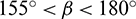(Fig. 14a). These bonds are approximately parallel or perpendicular to the shear direction. Under the action of shear displacement, either a large shear stress or a large tensile stress acts on these bonds. The shear strength of a bond is small if it is subjected to a large tensile stress (shear strength of the bond conforms to Mohr–Coulomb criterion in the PFC). So, those bonds either are subjected to a large shear stress or have a small shear strength. As a result, they are prone to fail caused by shear stress. However, the influences of on Rsp have a marked reduction with the increase of the Rh. For example, the Rsp of the sample with a D of 50 mm, a Rd of 0.3 and a Rh of 2.2 is always about 0.6 (Fig. 14e).

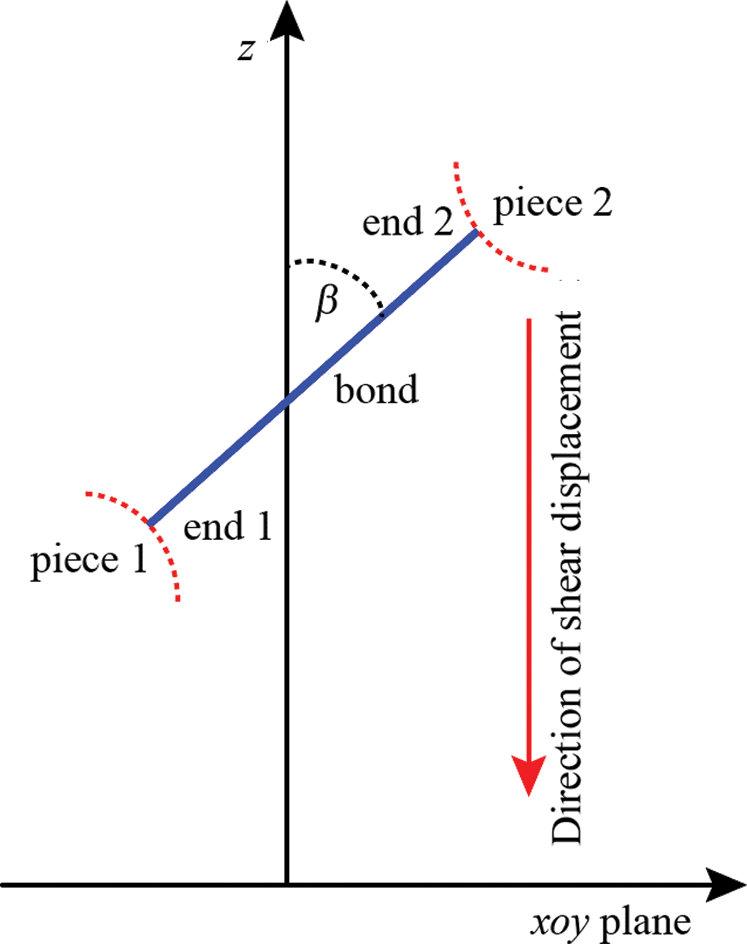
Figure 13: Schematic diagram of a bond in coordinate system

Figure 14: Change in Rc and Rs, in which the samples geometrical dimensions are D = 50 mm, Rd = 0.3 and (a) Rh = 0.6, (b) Rh = 1.0, (c) Rh = 1.4, (d) Rh = 1.8, (e) Rh = 2.2

4  Discussion

4.1 Normal Stress during Test

As shown in Fig. 15a sample used in the PST can be divided into two parts. Part I is the part outside the shear surface of the sample, which is a ring. Part II is the part within the shear surface of the sample. It can be known from Fig. 7 that the normal displacement increases with the increase of shear displacement, namely shear dilatancy occurs. Thus, the inner and outer diameters of Part I will grow during the test as the shear displacement increases due to shear dilatancy. Part I is subjected to tensile stress and tensile deformation in the direction perpendicular to the radial direction at any point. Additionally, Part I is subjected to compressive stress from Part II as well. Therefore, the actual normal stress on the shear surface is greater than zero in this study. If the PST is carried out under confining stress (normal stress) , the actual normal stress will be greater than . This can also be observed in Fig. 16, which shows the force chain of the contacts. When equals 0.6 , Part II is mainly subjected to compression while Part I is subjected to tensile in tangential direction and compressive stress in radial direction (Fig. 16a). With the increase of shear stress, the number of the contacts subjected to tensile stress grows. When is equal to , Part I is mainly subjected tensile stress (Fig. 16c). Thus, the disk looks like a rubber band (Part I) on a cylinder (Part II). The rubber band is stretched and applies a pressure on the cylinder. However, when the shear stress reaches its peak value, as shown in Fig. 10, macro-cracks within Part I in the radial direction have formed. At this moment, a portion of the tensile and compressive stress that Part I is subjected to in the tangential and radial directions have been released. As we know, shear strength under direct shear test is positively correlated with normal stress. Thus, the shear strength obtained by the PST will be larger than the actual shear strength, but the specific difference between the PST and real shear strength is uncertain, so further research is needed.

Figure 15: Stress state of a disk in the PST

Figure 16: Force chain of the disk with D = 50 mm, Rd = 0.3 and Rh = 1.0 under (a) , (b) and (c)

4.2 Recommended Disk Geometric Dimension

Fig. 5 gives the shear strength of sample with different D, Rd and Rh. When the Rd or Rh is small, shear strength is sensitive to all the three geometric parameters. Additionally, the shear dilatancy angles (Fig. 9) and peak shear failure rate (Fig. 12) also show a great difference. Thus, in the PST, samples with a small Rd (less than 0.3) and Rh (less than 1.4) is not recommended. When the Rd is greater than 0.6, the D has little influence on the shear strength which changes little and approaches a threshold value. However, if a sample has a Rd approaching 1.0, a too small Rh, or a too large D, it will make the Part II of the sample in Fig. 15 more likely to bend or break as shown in Fig. 10. In addition, a larger Rh leads to the sample cracking from one end to the other rather than from both ends to the middle (as shown in Fig. 10, row E). From this study, the sample size that should be used for the PST should be of a D between 50 and 70 mm, a Rd between 0.45 and 0.6, and a Rh between 1.4 and 1.8. Therefore, we suggest using samples with a D of about 60 mm, a Rd of about 0.5 and a Rh of about 1.6 to carry out the PST.

5  Conclusions

The PST has been used by researchers to determine the shear mechanical parameters of rocks. However, there are no suggested sample geometric dimensions at present. Simulations using PFC3D were carried out to investigate the influences of sample geometric dimensions on shear behaviors in the PST. We found that:

1.    When the ratio between sample Di and D or the ratio between sample H and Di is small, shear mechanical parameters of samples, such as shear strength, shear stiffness, dilatancy angles, and shear failure rate are sensitive to the sample geometric dimensions.

2.    In the PST, a cylindrical shear surface will be formed. If the disk height is comparatively small or the diameter of the surface is comparatively larger, the sample can easily produce a tensile fracture within the shear surface. Samples with a small ratio between sample H and Di cracks from both ends towards the middle while it cracks from one end to the other end for the samples with a large ratio between sample H and Di.

3.    In the PST, the actual normal stress is greater than the set value, which results in larger shear strength. The suggested sample geometric dimensions are given as a D of 60 mm, a ratio between sample Di and D of 0.5, and a ratio between sample H and Di of 1.6.

Funding Statement: This work is supported by the Fundamental Research Funds for the Central Universities, CHD (Nos. 300102210307, 300102210308), the National Natural Science Foundation of China (Nos. 51708040, 41831286, 51678063, 51978065).

Conflicts of Interest: The authors declare that they have no conflicts of interest to report regarding the present study.

This work is licensed under a Creative Commons Attribution 4.0 International License, which permits unrestricted use, distribution, and reproduction in any medium, provided the original work is properly cited.