DOI: 10.32604/cmes.2021.013982
ARTICLE
Characteristic and Thermal Analysis of Permanent Magnet Eddy Current Brake
School of Mechanical Engineering, Nanjing University of Science and Technology, Nanjing, 210094, China
*Corresponding Author: Guolai Yang. Email: yangglnjust@gmail.com
Received: 27 August 2020; Accepted: 09 December 2020
Abstract: In this paper, the subdomain analysis model of the eddy current brake (ECB) is established. By comparing with the finite element method, the accuracies of the subdomain model and the finite element model are verified. Furthermore, the resistance characteristics of radial, axial, and Halbach arrays under impact load are calculated and compared. The axial array has a large braking force coefficient but low critical velocity. The radial array has a low braking force coefficient but high critical velocity. The Halbach array has the advantages of the first two arrays. Not only the braking force coefficient is large, but also the critical speed is high. The parameter analysis of the Halbach array is further carried out. The inner tube thickness and air gap length are the sensitive factors of resistance characteristics. The demagnetization effect is significantly enhanced by the increase of the inner tube thickness. In order to ensure that the ECB does not overheat, the electromagnetic-thermal coupling model is established based on the heat transfer theory. The temperature rise of the inner tube is obvious while that of the permanent magnet is small. The temperature rise of the inner tube is more than 20 K each time, and that of the permanent magnet is less than 1 K each time.
Keywords: Eddy current brake; Halbach array; resistance characteristic; temperature rise
Compared with the traditional viscous and viscoelastic dampers, the ECB operates without direct contact between the primary and secondary, does not depend on friction, and has no working fluid. The structure of ECB is simple and reliable. The ECB has high performance, good durability, easy maintenance, long working life, and other advantages [1–5].
The ECB can be divided into rotary type and linear type according to the motion form of the mover, and the rotary type can be classified as radial and axial. Shin et al. [6] predicted the performance of the radial ECB through the layered theory approach. The experimental data showed that the measured value was slightly lower than the predicted value of the analytical model due to the influence of temperature rise. However, there was no further analysis of the heat transfer process of the ECB. Kou et al. [7] also used layered theory to predict the performance of linear ECB. The source term was replaced by equivalent current sheet, but this alternative approach may reduce the accuracy of the model [8]. Mehmet et al. [9] obtained the torque/speed equation of axial ECB based on curve fitting. However, the accuracy of this method depends on the original data. Shan et al. [10] proposed an approximate analysis method of eddy current force based on quasi-static assumption. Similar to other approximation methods, the undetermined coefficients come from the original data (numerical simulation or experiment), and the parameters need to be re-identified for different topologies. Wang et al. [11] regarded the reaction flux of eddy current as a leakage flux and derived a magnetic equivalent circuit (MEC) based formula for calculating the torque of axial eddy current coupler. In a considerably wide range of slip speeds, the torque predicted by this method is in good agreement with the results measured by finite element method and experiment. Nevertheless, obvious deviation appears as the slip speed exceeds the critical speed. Yang et al. [12] established a performance prediction model for radial eddy current coupler using a similar method. Liu et al. [13] combined Faraday’s law with the MEC model and proposed an analytical method for calculating the transfer torque of axial eddy current coupler. In order to characterize the eddy current reaction, an empirical value is fitted according to the finite element results. Bae et al. [14] established an analytical model of the permanent magnet movement in the copper tube applying the Biot-Savart law and verified the accuracy of the model through experiments. Since the effect of eddy current was not considered, the analytical model and the test results only coincided with the low speed. Ebrahimi et al. [15–17] proposed a modeling method of an ECB for vehicle suspension systems considering the skin effect on the basis of Bae. Then a prototype was made to compare the results of the analytical model and the simulation model. But only the braking force at low speed was compared. Amjadian et al. [18,19] investigated an ECB for seismic hazard mitigation of structures. The seismic performance of the proposed ECB is comparable with that of a passive magnetorheological damper of the same force capacity, but the cost is much lower. Ao et al. [20] developed and studied ECB as an alternative to viscous dampers. The ECB characteristics were evaluated by a finite element model and used for pedestrian bridge structures. Elejabarieta et al. [21] discussed an ECB used to attenuate structural vibration and proposed a new inverse method to numerically determine the dynamic properties of the ECB. The method based on a linear viscous force was validated by a practical application. Hua et al. [22] established an analytical model of an ECB based on surface charge and linear assumption. The analytical model was only valid for a limited range of low velocity and was verified by an experiment of a prototype mounted in a laboratory steel frame.
At present, the research of ECB is mostly used to suppress structural vibration or transfer torque as a coupler. A lot of research has been done on radial, axial, and linear plate ECB, but the research on tubular linear ECB is rare. It is a promising research direction to apply ECB to the braking of impact load. Under the impact load, the working speed of ECB will be relatively large, and the reliability requirement is higher. Compared with rotary ECB, linear ECB does not need an intermediate mechanical conversion device, and its structure is simpler and more reliable, especially suitable for high-speed operation. In addition, braking the impact load puts forward higher requirements for the energy consumption density of ECB. Compared with the linear plate ECB, there is no transverse end effect in the tubular linear ECB, so the permanent magnet utilization rate is high and the magnetic leakage is small, which can effectively improve the energy consumption density. However, due to its closed structure, the heat dissipation is poor. The change of temperature will change the constitutive relationship of the material and affect the performance of ECB. Therefore, the temperature change of ECB is a problem worthy of attention. Especially for the ECB with high energy consumption, it is necessary to conduct thermal analysis on the ECB.
In this paper, the tubular linear ECB is applied to the braking of impact load. The braking force characteristics of the axial array, radial array, and Halbach array under impact load are investigated to select the permanent magnet array suitable for impact load braking. The influence of design parameters on the braking force characteristics is further studied, which provides a valuable reference for the design of ECB. In order to prevent the ECB from overheating, the electromagnetic thermal field coupling model is established to study the transient heat transfer process.
The structure of the tubular linear ECB for impact load braking is shown in Fig. 1. A permanent magnet array is mounted on the shaft and guided by guide rings for linear motion. One end of the shaft is connected with the moving part. The secondary consists of an inner tube and an outer tube. The inner tube can be made of copper or aluminum alloy with high conductivity, and the outer tube can be made of pure iron or carbon steel to enhance the magnetic flux density.
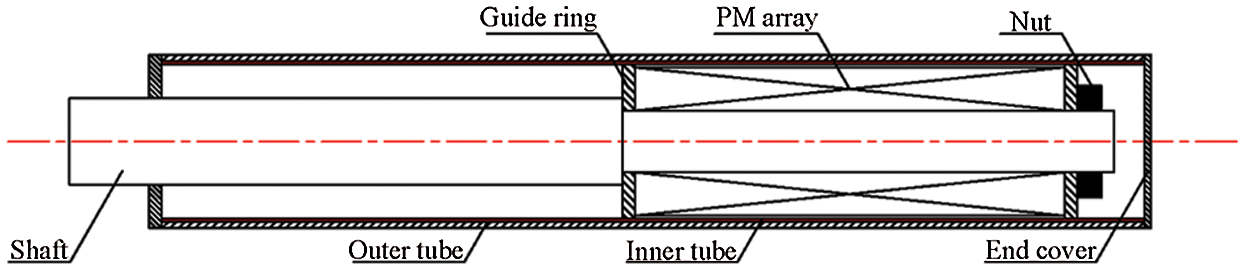
Figure 1: Schema of tubular linear ECB
For tubular linear ECB, radial array, axial array, or Halbach array are mainly used. Fig. 2 shows these three arrays The Halbach array is first proposed by Halbach [23]. The radial and axial arrays are combined according to a certain rule. The magnetic field lines on one side of the array are converted to increase the flux density and decrease the flux density on the other side.
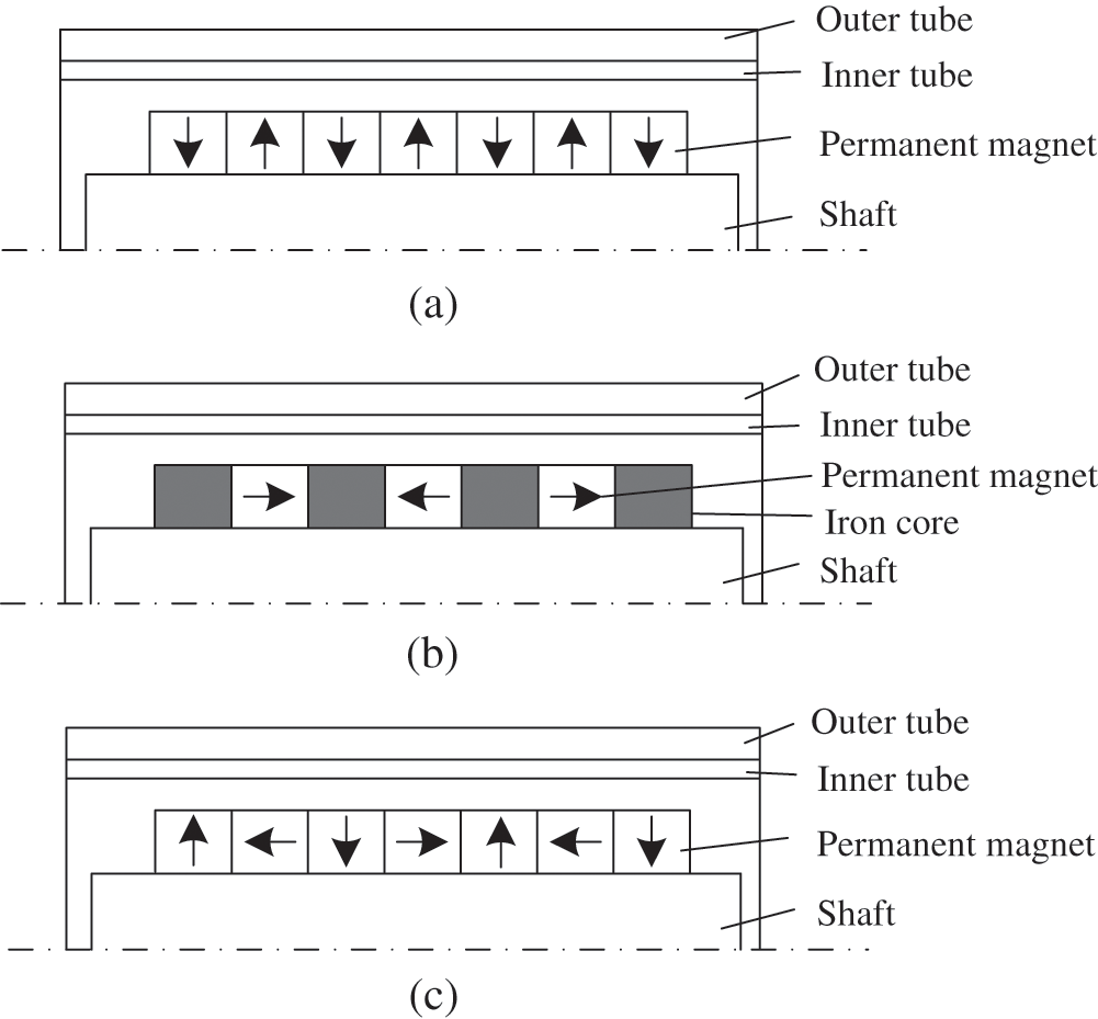
Figure 2: Three types of permanent magnet arrays. (a) Radial array, (b) Axial array, (c) Halbach array
When the relative motion between primary and secondary occurs, the secondary cuts the magnetic force lines formed by the primary, thereby generating dynamic electromotive force. Under the action of the dynamic electromotive force, and charges move directionally, forming an eddy current. The interaction between the eddy current and the magnetic field generates the Lorentz force, which hinders the relative motion of the two. From the perspective of energy conversion, the mechanical energy is first converted into electrical energy, then converted into thermal energy through resistance for dissipation.
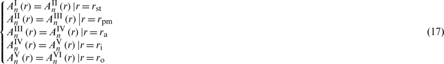
The quasi-static analytical model of ECB can be established by subdomain technology. Taking the Halbach array as an example, Fig. 3 is the simplified subdomain model. The simplified subdomain model includes the following assumptions: The constitutive relationship of ferromagnetic materials is linear; the electromagnetic field is periodically distributed along the z axis, that is, the longitudinal end effect is ignored; the current density distribution is only oriented along the z axis to simplify the model to a two-dimensional problem. The cylindrical coordinate system is fixed on the Halbach array. ro, ri, ra, rpm and rst are the outer radii of the outer tube, inner tube, air gap, permanent magnet, and support rod, respectively. b and c are the axial length of axial magnetization and radial magnetization of the permanent magnets.  is the pole pitch. hm,
  and d are the radial thickness of permanent magnets, air gap, and inner tube, respectively.
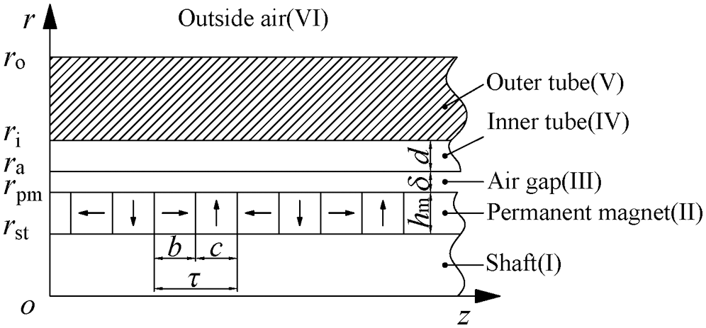
Figure 3: Simplified subdomain model
The analytical model is divided into six subdomains.
Subdomain I: Shaft. Assuming that the conductivity is zero, the permeability is the same as air.
Subdomain II: Permanent magnet. Assuming that the conductivity is zero, the permeability is the same as air.
Subdomain III: Air gap.
Subdomain IV: Inner tube. High conductivity, permeability is the same as air.
Subdomain V: Outer tube. Ferromagnetic material, assuming that the constitutive relationship is linear.
Subdomain VI: Outside air.
Applying Maxwell’s equations and magnetic vector potential, the governing equation can be expressed as:

where A is magnetic vector potential.  is the permeability of vacuum and
  is the relative permeability. J denotes the current density.
Since the conductivity of subdomains I, III and VI is zero, the governing equation can be simplified as the Laplace equation.

The constitutive relation of the permanent magnet can be described by residual magnetism


where  ,
,  , and
, and  are the magnetic flux density, remanence, radial remanence, and axial remanence, respectively. Fig. 4 shows the distribution of remanence. Bres0 is the value of the residual magnetism.
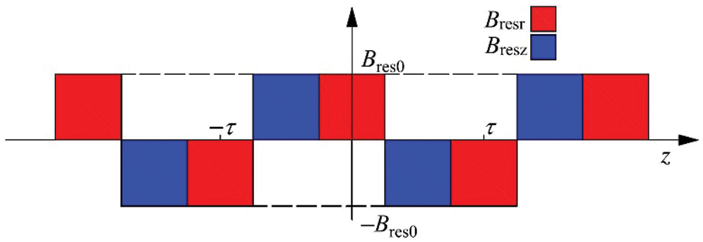
Figure 4: Distribution of remanence
The distribution of remanence can be expressed by the Fourier series.
where  .
.
Substitute (5) into (1), and based on the assumption that the conductivity of the permanent magnet is zero. The governing equation of Subdomain II can be written as:

According to Ohm’s Law and Faraday’s Law


The governing equation of Subdomain IV and V are derived as:

where  is the conductivity. v is the relative speed of primary and secondary.
According to the assumption, all electromagnetic quantities have a period of  . So the magnetic vector potential A can be separated by variables as

Substitute (10) into (2), (6), and (9), the ordinary differential equations in each subdomain are


Solving the above ordinary differential equation to obtain the general solution of each subdomain which is


where  ,
,  ,
,  , and
, and  are the first-order modified Bessel functions of the first and the second kind and the first-order modified Struve function, respectively.
  and
and  are unknown constants depending on the following boundary conditions.
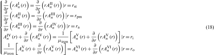


The normal component of magnetic flux density on the interface is continuous, guaranteed by (17). And (18) indicates that the tangential component of the magnetic field strength on the interface is continuous. Eqs. (19) and (20) are natural boundary conditions, (19) is obtained from the symmetry of cylindrical coordinate. The magnetic flux density is obviously zero at infinity.
Analytical expressions of the magnetic flux density and eddy current density of Subdomain IV and V can get as:


Finally, the Lorentz force can be calculated

The accuracy of the subdomain model will be verified by comparing it with the finite element model. The calculations are performed using the parameters given in Tab. 1.
Table 1: Parameters of the ECB used in the calculations
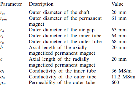
Fig. 5 shows the radial flux density distribution (r = (ra + ri/2) calculated by the analytical method and finite element method. It can be found that with the increase of speed, the distribution of magnetic flux density is distorted under the reaction of eddy current. Without considering the magnetic saturation, the analytical method is in good agreement with the finite element method. The relative error is controlled within 2.9%. Considering the magnetic saturation, the radial flux density decreases. Fig. 6 compares the eddy current density at different locations in the inner tube (r = (ra + ri)/2). Similar to Fig. 5, the analytical method result fits the finite element method result very well. The relative error is less than 3.38%.
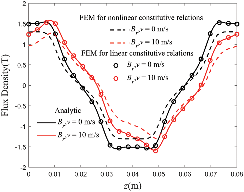
Figure 5: Comparison of magnetic flux density as functions of z at r = (ra + ri)/2
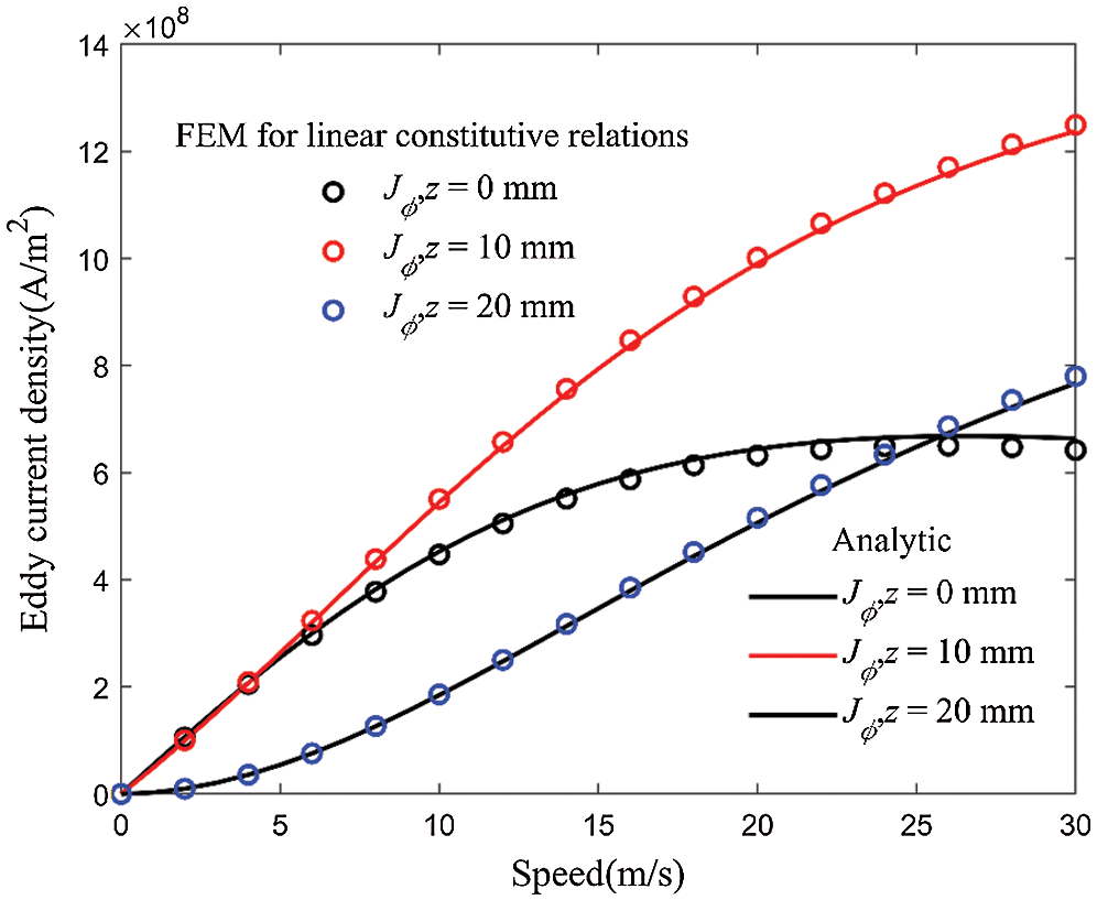
Figure 6: Comparison of current density as functions of v at different points
The results of the subdomain method and the finite element method are shown in Fig. 7. It can be seen that the calculation results of the subdomain method and the results of the finite element method are in good agreement, and the relative error is less than 1.28%. In the subdomain model, the constitutive relationship of the ferromagnetic material is assumed to be linear, with the magnetic saturation being ignored. In practical applications, the phenomenon of magnetic saturation exists. After the constitutive relationship of the ferromagnetic material being set as nonlinear, the magnitude of the braking force is reduced compared with the former. As the speed exceeding 15 m/s, the higher the speed, the more obvious the decrease of braking force, because the magnetic saturation phenomenon is more significant.
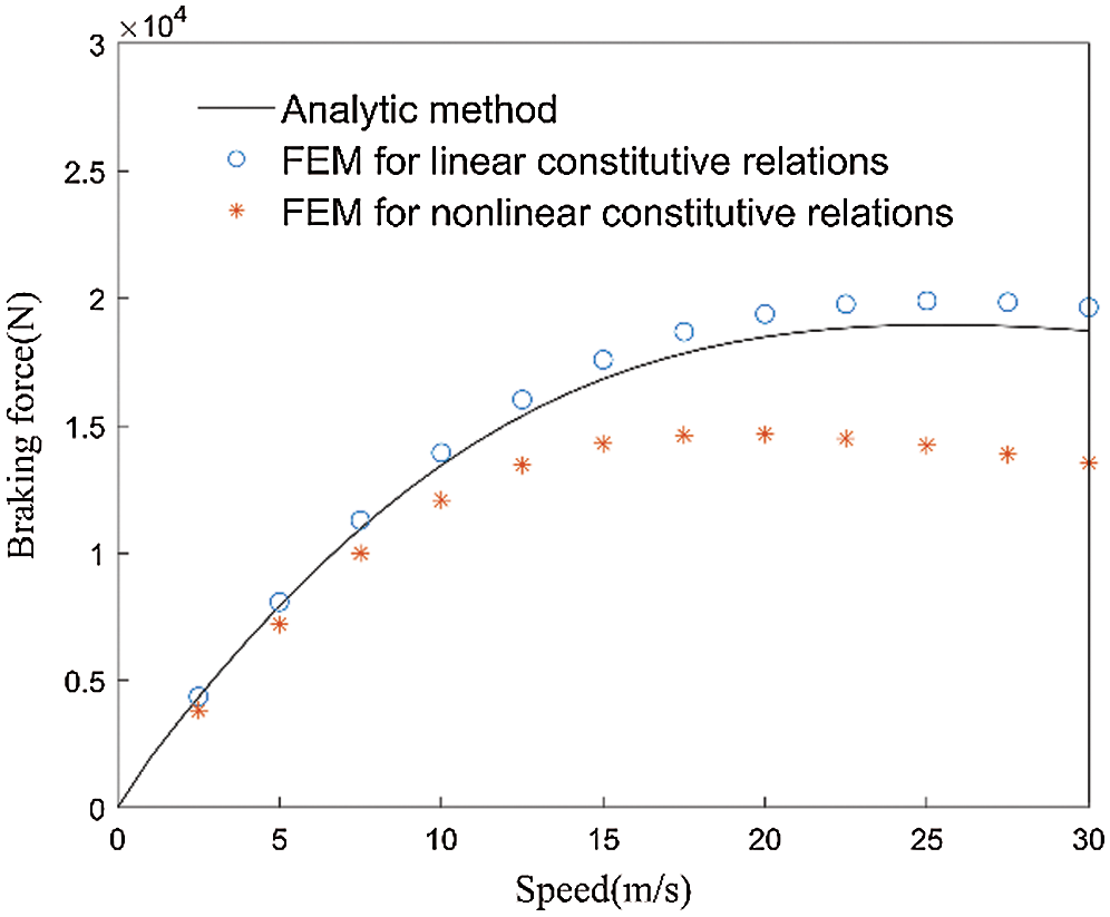
Figure 7: Comparison of braking force as functions of v
The main advantage of the subdomain model is the lower computational cost and high accuracy. However, it has some important disadvantages that limit its applicability. First, the complexity of the method depends on the number of subdomains, and boundary conditions of the subdomains must be simple. This makes it difficult to apply machines with complex geometric structures. The second is that this method is only applicable to quasi-static electromagnetic fields. The third is that the method assumes that the material’s constitutive relationship is linear. Although it is possible to calculate the nonlinear constitutive relationship through iteration, it will undoubtedly increase the calculation time greatly [24].
According to the calculation results of the subdomain model and the finite element model, the accuracy of the subdomain model and the finite element model are verified. The ECB studied in this paper has a very rapid speed change under the action of an intensive impact load, so it must be studied as a transient field. In addition, there is magnetic saturation. Therefore, the following sections will use the finite element method as the main research method.
3 Performance Analysis of three types of ECB
The relationship between braking force and speed of different arrays are shown in Fig. 8. Different arrays have the same basic rules. In the low speed stage (speed be less than 2 m/s), the braking force is linearly related to the speed. As the speed increases, due to the demagnetization effect, the braking force is no longer linearly related to the speed, and there is a peak value. The speed at which the braking force reaches its peak value is called the critical speed. When the speed exceeds the critical speed, the braking force decreases as the speed increases. It can be seen from Fig. 8 that the critical speed of the radial array is higher but the braking force coefficient (ratio of braking force to speed) in the low speed stage is small. The braking force coefficient of the axial array is significantly greater than that of the radial array, but its critical speed is only 12.4 m/s. The Halbach array has the advantages of both axial and radial arrays. The critical speed can reach 20.4 m/s. The braking force coefficient is equivalent to that of the axial array, and the peak braking force is significantly greater than that of the axial or radial array.
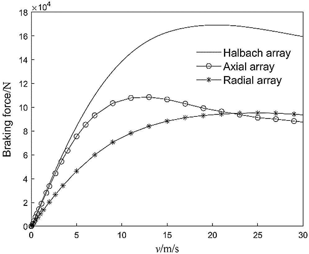
Figure 8: Braking force characteristics of ECB with different arrays
In order to compare the actual braking effect of different arrays of ECB, the transient braking process was calculated. The intensive impact load Fpt is shown in Fig. 9, with a duration of 0.01 s and a peak value of 2700 kN. The secondary motion law is controlled by the following formula:

where m is the mass of the moving part. Ff is the force of the recuperator. The function of the device is to store energy during the braking process. After the braking process is completed, the stored energy is used to reset the moving part. Ff is related to the braking distance as shown in Fig. 10.
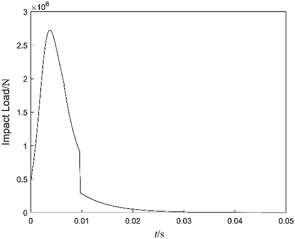
Figure 9: Curves of impact load
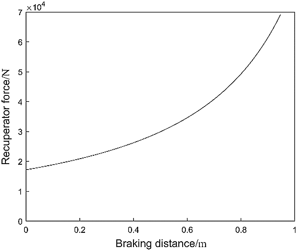
Figure 10: Curves of recuperator force
The braking force generated by the ECB during actual braking is shown in Fig. 11. The braking force generated by the Halbach array is significantly greater than that of axial and radial arrays. Its peak braking force reaches 164.4 kN, and the peak braking force of the radial array is only 89.2 kN. The braking force generated by the axial array rapidly decreases after reaching the peak. The reason is that under the intensive impact load, the working speed quickly reaches more than 15 m/s (see Fig. 12), which exceeds the critical speed of the axial array and produces a demagnetization effect. The critical speed of the Halbach array and radial array is relatively high, and the demagnetization effect is not obvious.
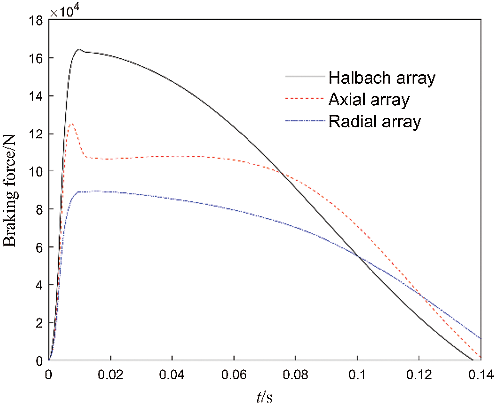
Figure 11: Curves of braking force
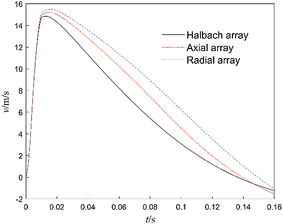
Figure 12: Curves of recuperator force
Fig. 13 shows the resultant resistance (braking force plus recuperator force) curve of the axial array, Halbach array ECB and hydraulic brake in actual work. The resultant resistance curve of the Halbach array is similar to the hydraulic brake resistance curve, the former is more stable. The resultant resistance generated by the axial array drops rapidly after reaching the first peak value due to the demagnetization effect. As the braking distance increases and the working speed decreases, the recuperator force continuously increases and the demagnetization effect decreases. The resultant resistance increases to form the second peak, and the resultant resistance curve forms an obvious saddle shape. The braking force generated by the radial array is too small to meet the working requirements.
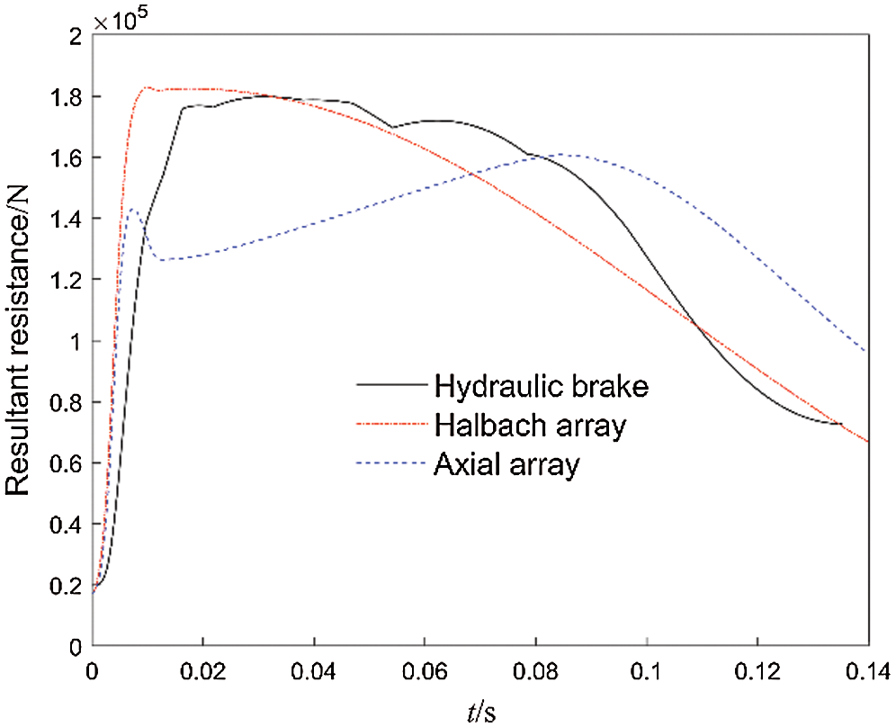
Figure 13: Curves of resultant resistance
Comparing the performance of the axial, radial, and Halbach arrays of the ECB, the Halbach array has advantages over both the axial array and the radial array. The braking force coefficient is large and the critical speed is high. In the same volume, the braking force provided by the Halbach array is much greater than that of the axial array and the radial array, the actual performance is the best.
4 Parameter Analysis of Halbach Array ECB
The performance of the ECB is affected by many parameters, such as the air gap distance, the thickness of the inner tube, the thickness of the outer tube, and the size of the permanent magnet. The analysis in the previous section shows that the performance of the Halbach array is better than axial or radial arrays. This section takes the Halbach array ECB as the research object, then analyzes in detail the effects of the outer tube thickness, inner tube thickness, and air gap distance on the performance of the ECB.
The distribution of magnetic induction lines of the static magnetic field of the Halbach array ECB is shown in Fig. 14a. Magnetic induction lines are converged by the radial magnetized permanent magnets and pass through the inner tube almost vertically. As the working speed v increases, the original static magnetic field is affected by the magnetic field generated by the eddy current. The distribution of magnetic induction lines is distorted and no longer passes vertically through the inner tube as shown in Fig. 14b.
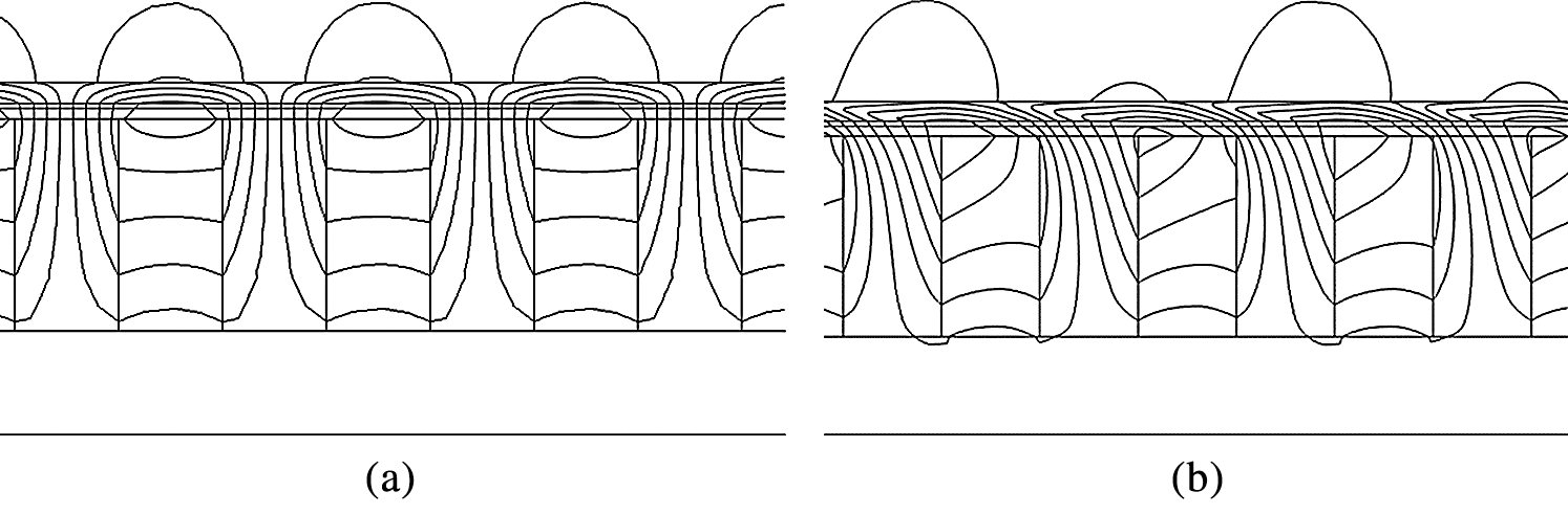
Figure 14: Local static magnetic field. (a) Static magnetic field (b) Magnetic field at the speed of 20 m/s
Fig. 15 is the air gap magnetic flux density under different outer tube thickness. It can be seen from the figure that the air gap magnetic flux density increases with the increase of the outer tube thickness. With the further increase of the outer tube thickness, the air gap magnetic flux density no longer increases significantly. When the outer tube thickness exceeds 8 mm, increasing the outer tube thickness has almost no effect on increasing the air gap magnetic flux density.
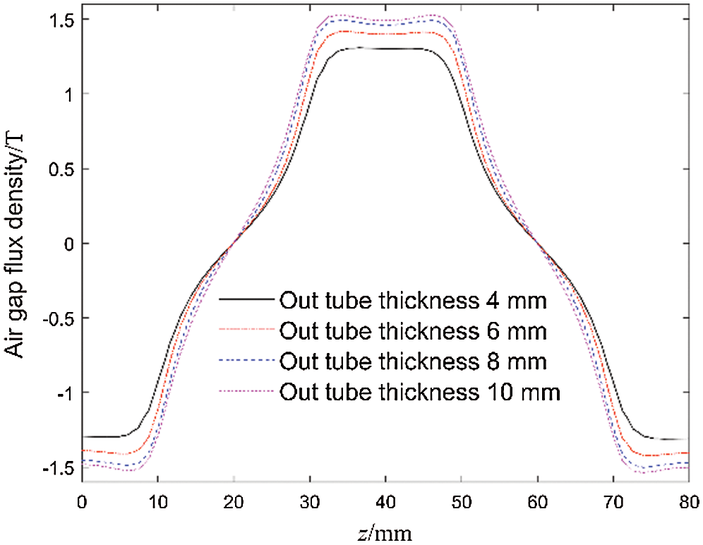
Figure 15: Air gap magnetic flux density with different outer tube thicknesses
The resultant resistance curves of the ECB under different outer tube thicknesses are shown in Fig. 16. The greater the thickness of the outer tube, the greater the air gap magnetic flux density, which makes the ECB with greater braking force at the same working speed. But the critical speed will decrease and the demagnetization effect will increase. Fig. 17 shows resultant resistance curves of the ECB under different inner tube thickness. As the thickness of the inner tube increases, the area where eddy currents are generated in the inner tube increases, so the braking force coefficient increases. But the demagnetization effect is significantly enhanced. Although increasing the thickness of the inner tube can obtain greater resultant resistance at low speeds, due to the working speed exceeding the critical speed, the significant demagnetization effect instead causes the braking effect to deteriorate. As shown in Fig. 17, the demagnetization effect is very obvious when the thickness of the inner tube reaches 2 mm and more, and the resultant resistance curve forms an obvious saddle shape.
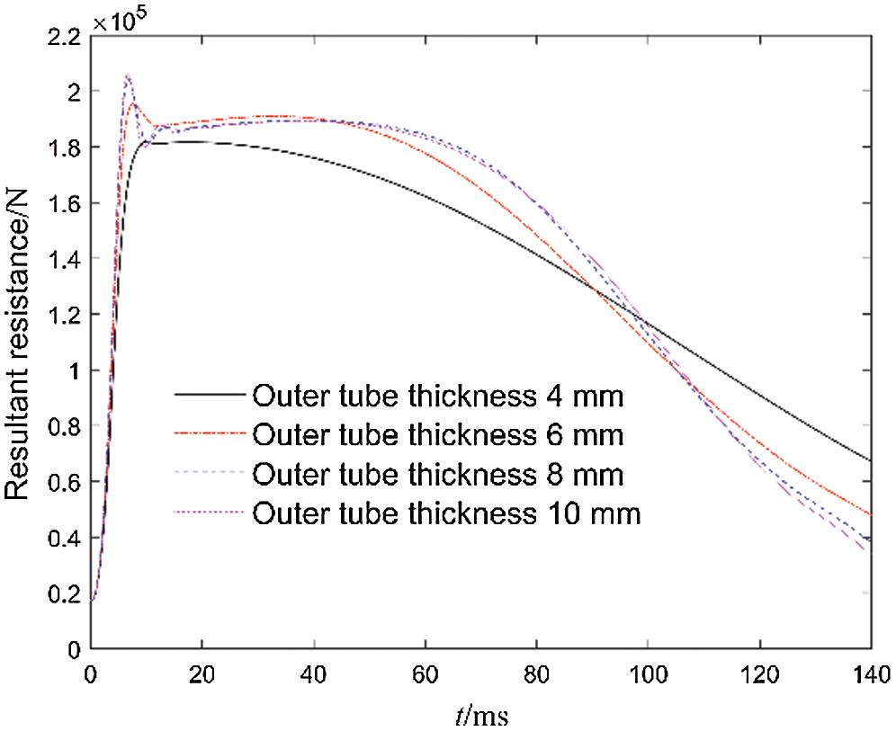
Figure 16: Curves of resultant resistance with different outer tube thicknesses
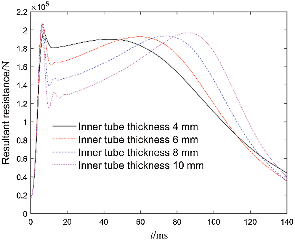
Figure 17: Curves of resultant resistance with different inner tube thicknesses
Air gap distance is a critical parameter. The air gap magnetic flux density is closely related to the air gap distance. As shown in Fig. 18, as the air gap distance increases, the magnitude of the resultant resistance decreases significantly. The air gap distance is mainly constrained by the shape tolerances and position tolerances of the support rod, permanent magnet, inner and outer tubes, as well as manufacturing and assembly tolerances. Therefore, the air gap distance is determined according to actual performance requirements and processing and assembly costs.
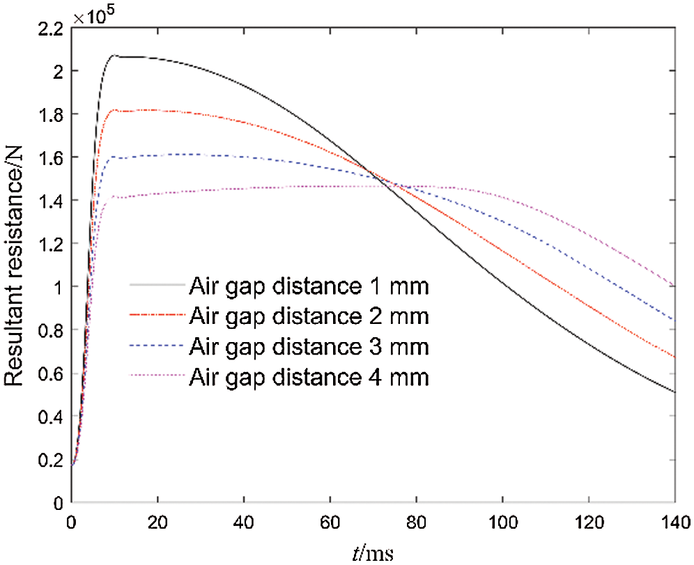
Figure 18: Curves of resultant resistance with different air gap distance
As mentioned in the first section, the kinetic energy of the moving part is finally converted into thermal energy dissipation. Temperature changes will change the conductivity of the inner tube, the conductivity and permeability of the outer tube, and the performance of the permanent magnet. When the temperature exceeds the Curie temperature of the permanent magnet, it will cause irreversible loss of the permanent magnet and seriously affect the performance of the ECB. In this section, the electromagnetic-thermal coupling model is established based on the heat transfer characteristics of the ECB, then the thermal field of the ECB is calculated.
The heat source of the ECB is mainly concentrated in the inner tube. The heat is dissipated by the forced convection of the air gap between the primary and secondary, heat conduction inside the inner and outer tubes, and natural convection on the outer surface of the outer tube. The control equation of convection heat dissipation is shown in Eqs. (26)–(28).


where q is the heat dissipation capacity per unit area, h is the heat transfer coefficient,  is the temperature variation on the heat exchange surface, Nu is the Nusselt number,
  is the heat conductivity coefficient of air, and l is the characteristic size.
The primary and secondary form a concentric annular space (air gap). This annular space can be assumed to perform forced convection heat transfer when the ECB is in operation. The Reynolds number determines the state of forced convection (laminar or turbulent flow) in the air gap. The Reynolds number can be calculated by the following formula:

where vg and  are the speed and kinematic viscosity of air, respectively, the critical Reynolds number is 2300. Taking the maximum working speed to calculate the Reynolds number in the annular space is 1912.4. Since the Reynolds number is lower than the critical value, the flow state is assumed to be laminar. The Nu number in the annular space with fully developed forced convective heat transfer is 5.385 [25].
The outer surface of the outer tube is in natural convective heat transfer in a large space. The Nu number can be obtained from the relevant empirical equations [26].

where C and m are constants and are related to the surface shape and flow state. Pr is the Prandtl number of air. Gr is Grashof number, its role in natural convection is equivalent to that of Reynolds number in forced convection. The mathematical expressions of Pr and Gr are


where a is the thermal diffusion coefficient of air, g is the acceleration of gravity, and  is the coefficient of volume change.
At standard atmospheric pressure, the Pr and Gr of the air at 25  can be calculated as 0.722 and
  , respectively. Consulting the literature [25], it can get that constant C = 0.53, m = 1/4. Therefore, the Nu number of natural convection heat transfer on the outer surface is 30.46. The heat transfer coefficient h of each surface can be obtained by (27).
The eddy current calculated by the electromagnetic field is used as the heat source of the thermal field, boundary conditions of the thermal field are set according to the obtained heat transfer coefficient, and the ambient temperature is set as 298.15 K, then the temperature change of the ECB is solved.
Fig. 19 shows temperature variation curves of different points on the surface of the inner tube. The z of the initial recoil position is zero. When the ECB works, the moving part moves from the initial position to the end position in the inner tube. Only the middle part of the inner tube is always in a working state. The working time of both ends of the inner tube is shorter and the temperature rise is lower.
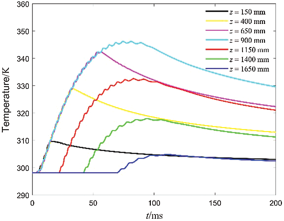
Figure 19: Curves of resultant resistance with different air gap distance
Curves of the maximum temperature of the ECB and the maximum temperature of the permanent magnet are shown in Fig. 20. The calculation results show that the highest temperature appears in the inner tube, and the highest temperature is 346.86 K. The temperature change of the permanent magnet is not obvious, which is less than its maximum working temperature of 353.15 K.
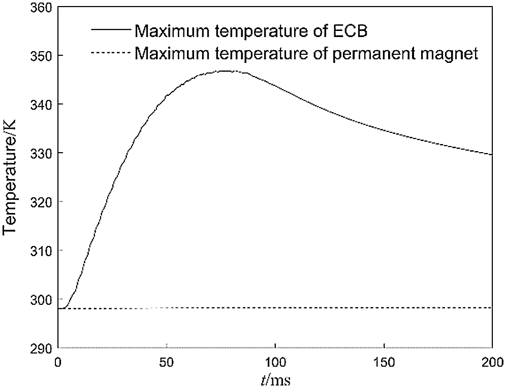
Figure 20: Curves of resultant resistance with different air gap distance
Assume that the ECB runs 8 times per minute, so the working interval is 7.5 s. The thermal field result of the previous work is used as the initial condition for the calculation of the next thermal field. The calculated maximum temperature change curve of the ECB with the continuous operation is shown in Fig. 21. The maximum temperature of the inner tube and permanent magnet changes with each operation as shown in Tab. 2. The first working temperature rise of the inner tube is 22 K, then each time the temperature rise slightly decreases. The reason is that the temperature of the ECB is increased, the temperature difference with the air is increased, and the heat dissipation ability of the outer surface is enhanced. Since the permanent magnet is not directly connected to the inner tube, the temperature rise of the permanent magnet is not obvious. However, as the temperature difference increases, the temperature rise of each permanent magnet gradually increases. Fig. 22 is the temperature distribution at 7.5 s, which is also the initial condition of the second operation.
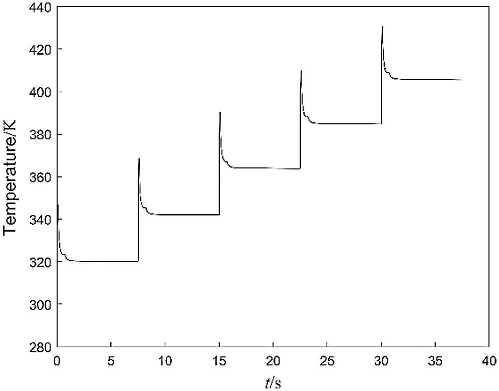
Figure 21: Curves of maximum temperature for continuous working
Table 2: Temperature rise continuous working
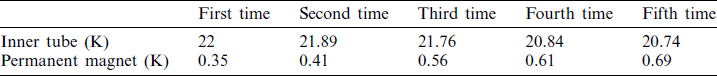
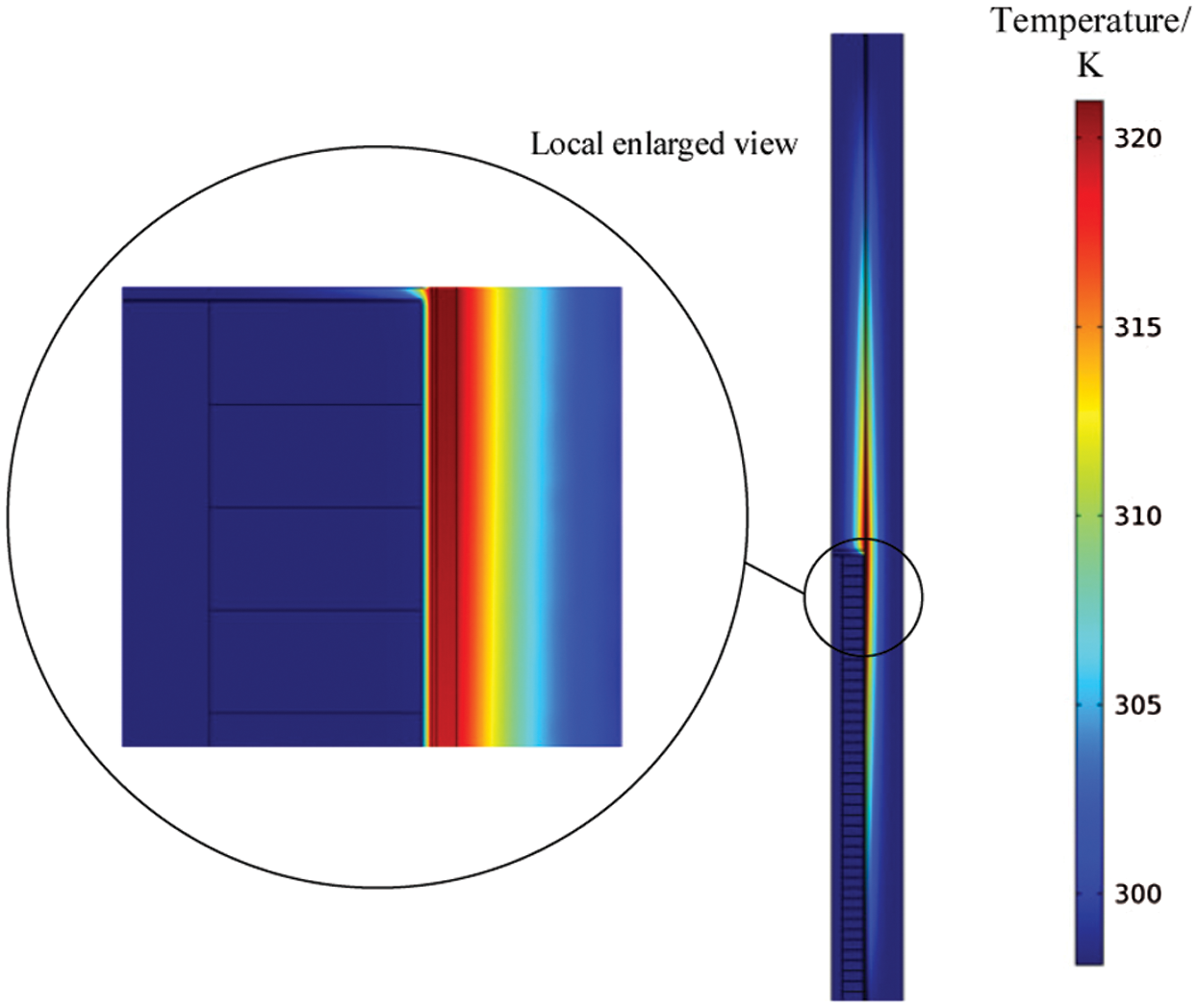
Figure 22: Temperature distribution on 7.5 s
This paper analyzes the resistance characteristics of three types of ECB. The parameter analysis of the Halbach array ECB is further conducted. Finally, the electromagnetic-thermal field coupling model is established, then the temperature change of the ECB is calculated. The main conclusions are as follows:
1. Braking force calculated by the subdomain model and the finite element model are in good agreement, assuming that the constitutive relationship of ferromagnetic material is linear. However, the actual braking force is lower than the braking force calculated by the linear assumption due to magnetic saturation.
2. Compared with radial array and axial array, Halbach array permanent magnet ECB has advantages of large braking force coefficient and high critical speed.
3. Increasing the thickness of the inner or/and outer tubes will increase the braking force coefficient and decrease the critical speed. Under the game between these two indicators, there is an optimal value for the thickness of the inner and outer tubes. The smaller the air gap distance, the higher the air gap magnetic flux density.
4. The highest temperature appears in the inner tube, and the temperature of the permanent magnet does not change much. Assuming that the working interval is 7.5 s, the temperature of the inner tube rises about 21 K each time it works.
In the future, experimental studies can be carried out to verify the accuracy of the model in this paper. During continuous operation, the temperature rise of ECB is obvious. It is a meaningful and interesting research work to add a cooling system to the original structure.
Funding Statement: This work was supported by the National Natural Science Foundation of China (Grant No. 51705253).
Conflicts of Interest: The authors declare that they have no conflicts of interest to report regarding the present study.
1. Chen, C., Xu, J., Yuan, X., Wu, X. (2019). Characteristic analysis of the peak braking force and the critical speed of eddy current braking in a high-speed maglev. Energies, 12(13), 2622. DOI 10.3390/en12132622. [Google Scholar] [CrossRef]
2. Cho, S., Liu, H. C., Ahn, H., Lee, J., Lee, H. W. (2017). Eddy current brake with a two-layer structure: Calculation and characterization of braking performance. IEEE Transactions on Magnetics, 53(11), 1–5. DOI 10.1109/TMAG.2018.2792846. [Google Scholar] [CrossRef]
3. Lubin, T., Vahaj, A. A., Rahideh, A. (2020). Design optimisation of an axial-flux reluctance magnetic coupling based on a two-dimensional semi-analytical model. IET Electric Power Applications, 14(5), 901–910. DOI 10.1049/iet-epa.2019.0746. [Google Scholar] [CrossRef]
4. Takahashi, K., Tsukima, M., Kai, T., Nakagawa, T. (2017). A three-position swing electromagnetic actuator with an integrated eddy current brake for suppression of the operating time and improvement of the stopping accuracy. Electrical Engineering in Japan, 200(3), 44–51. DOI 10.1002/eej.22895. [Google Scholar] [CrossRef]
5. Yang, P., Zhou, G., Zhu, Z., Tang, C., He, Z. et al. (2019). Linear permanent magnet eddy current brake for overwinding protection. IEEE Access, 7, 33922–33931. DOI 10.1109/ACCESS.2019.2902892. [Google Scholar] [CrossRef]
6. Shin, K. H., Park, H. I., Cho, H. W., Choi, J. Y. (2018). Semi-three-dimensional analytical torque calculation and experimental testing of an eddy current brake with permanent magnets. IEEE Transactions on Applied Superconductivity, 28(3), 1–5. DOI 10.1109/TASC.2018.2795010. [Google Scholar] [CrossRef]
7. Jin, Y., Li, L., Kou, B., Pan, D. (2019). Thermal analysis of a hybrid excitation linear eddy current brake. IEEE Transactions on Industrial Electronics, 66(4), 2987–2997. DOI 10.1109/TIE.2018.2847703. [Google Scholar] [CrossRef]
8. Atallah, K., Zhu, Z. Q., Howe, D. (1998). Armature reaction field and winding inductances of slotless permanent-magnet brushless machines. IEEE Transactions on Magnetics, 34(5), 3737–3744. DOI 10.1109/20.718536. [Google Scholar] [CrossRef]
9. Gulbahce, M. O., Kocabas, D. A. (2017). A comprehensive approach to determining the speed/torque relationships of eddy current brakes. Electrical Engineering, 100(3), 1579–1587. DOI 10.1007/s00202-017-0636-x. [Google Scholar] [CrossRef]
10. Loong, C. N., Shan, J., Shi, Z., Chang, C. C. (2020). Approximate analysis of eddy-current force under time-varying velocity motion for structural control. Journal of Sound and Vibration, 475, 115295. DOI 10.1016/j.jsv.2020.115295. [Google Scholar] [CrossRef]
11. Wang, J., Zhu, J. (2018). A simple method for performance prediction of permanent magnet eddy current couplings using a new magnetic equivalent circuit model. IEEE Transactions on Industrial Electronics, 65(3), 2487–2495. DOI 10.1109/TIE.2017.2739704. [Google Scholar] [CrossRef]
12. Yang, X., Liu, Y. (2019). An improved performance prediction model of permanent magnet eddy current couplings based on eddy current inductance characteristics. AIP Advances, 9(3), 35350. DOI 10.1063/1.5089183. [Google Scholar] [CrossRef]
13. Cheng, X., Liu, W., Zhang, Y., Liu, S., Luo, W. (2020). A concise transmitted torque calculation method for pre-design of axial permanent magnetic coupler. IEEE Transactions on Energy Conversion, 35(2), 938–947. DOI 10.1109/TEC.2019.2948974. [Google Scholar] [CrossRef]
14. Bae, J. S., Hwang, J. H., Park, J. S., Kwag, D. G. (2010). Modeling and experiments on eddy current damping caused by a permanent magnet in a conductive tube. Journal of Mechanical Science and Technology, 23(11), 3024–3035. DOI 10.1007/s12206-009-0819-0. [Google Scholar] [CrossRef]
15. Ebrahimi, B., Khamesee, M. B., Golnaraghi, F. (2009). Eddy current damper feasibility in automobile suspension: Modeling, simulation and testing. Smart Materials and Structures, 18(1), 15017. DOI 10.1088/0964-1726/18/1/015017. [Google Scholar] [CrossRef]
16. Ebrahimi, B., Khamesee, M. B., Golnaraghi, F. (2009). A novel eddy current damper: Theory and experiment. Journal of Physics D: Applied Physics, 42(7), 75001. DOI 10.1088/0022-3727/42/7/075001. [Google Scholar] [CrossRef]
17. Ebrahimi, B., Khamesee, M. B., Golnaraghi, M. F. (2008). Design and modeling of a magnetic shock absorber based on eddy current damping effect. Journal of Sound and Vibration, 315(4–5), 875–889. DOI 10.1016/j.jsv.2008.02.022. [Google Scholar] [CrossRef]
18. Amjadian, M., Agrawal, A. K. (2017). A passive electromagnetic eddy current friction damper (PEMECFDTheoretical and analytical modeling. Structural Control and Health Monitoring, 24(10), e1978. DOI 10.1002/stc.1978. [Google Scholar] [CrossRef]
19. Amjadian, M., Agrawal, A. K. (2018). Modeling, design, and testing of a proof-of-concept prototype damper with friction and eddy current damping effects. Journal of Sound and Vibration, 413, 225–249. DOI 10.1016/j.jsv.2017.10.025. [Google Scholar] [CrossRef]
20. Ao, W. K., Reynolds, P. (2017). Analytical and experimental study of eddy current damper for vibration suppression in a footbridge structure. Dynamics of Civil Structures, 2, 131–138. DOI: 10.1007/978-3-319-54777-0_17. [Google Scholar] [CrossRef]
21. Irazu, L., Elejabarrieta, M. J. (2018). Analysis and numerical modelling of eddy current damper for vibration problems. Journal of Sound and Vibration, 426, 75–89. DOI 10.1016/j.jsv.2018.03.033. [Google Scholar] [CrossRef]
22. Huang, Z. W., Hua, X. G., Chen, Z. Q., Niu, H. W. (2018). Modeling, testing, and validation of an eddy current damper for structural vibration control. Journal of Aerospace Engineering, 31(5), 4018063. DOI 10.1061/(ASCE)AS.1943-5525.0000891. [Google Scholar] [CrossRef]
23. Halbach, K. (1980). Design of permanent multipole magnets with oriented rare earth cobalt material. Nuclear Instruments and Methods, 169(1), 1–10. DOI 10.1016/0029-554X(80)90094-4. [Google Scholar] [CrossRef]
24. Djelloul-Khedda, Z., Boughrara, K., Dubas, F., Ibtiouen, R. (2017). Nonlinear analytical prediction of magnetic field and electromagnetic performances in switched reluctance machines. IEEE Transactions on Magnetics, 53(7), 1–11. DOI 10.1109/TMAG.2017.2679686. [Google Scholar] [CrossRef]
25. Yang, S., Tao, W. (2006). Heat transfer. Higher Education Press, Beijing. [Google Scholar]
26. Xu, S. (2016). Heat transfer. Science Press, Beijing. [Google Scholar]
 | This work is licensed under a Creative Commons Attribution 4.0 International License, which permits unrestricted use, distribution, and reproduction in any medium, provided the original work is properly cited. |