Computer Modeling in Engineering & Sciences

DOI: 10.32604/cmes.2021.014405

ARTICLE

Classifying Abdominal Fat Distribution Patterns by Using Body Measurement Data

Jingjing Sun1, Bugao Xu1,2,*, Jane Lee3 and Jeanne H. Freeland-Graves3

1Department of Biomedical Engineering, University of Texas, Austin, TX 78712, USA
2Department of Computer Science and Engineering, University of North Texas, Denton, TX 76201, USA
3Department of Nutritional Sciences, University of Texas, Austin, TX 78712, USA
*Corresponding Author: Bugao Xu. Email: bugao.xu@unt.edu
Received: 24 September 2020; Accepted: 03 December 2020

1  Introduction

Obesity is a public health concern as it is associated with chronic diseases, such as type 2 diabetes, cardiovascular disease, and certain types of cancers [1–3]. Evidence suggests that body size and shape are important in predicting metabolic risk factors and their adverse effects [4–7]. Several anthropometric measurements, including body mass index (BMI), waist circumference (WC), and waist-hip ratio (WHR), are widely used to evaluate obesity due to their simplicity and low-cost. BMI is a convenient risk predictor for type 2 diabetes, hypertension and coronary heart disease [8]. WC exhibits significant predictive power for metabolic diseases [4,9], and WHR is an independent risk factor for stroke [10]. Although anthropometric measurements are standard parameters for obesity evaluation, the accuracy and efficacy of these simple measurements are often questioned [11], because these manual measurements have inherent errors that weaken the intra- and inter-observers’ reliability [12] and some of them are not strongly related to adiposity conditions of an individual [7]. Traditional parameters (BMI, WHR and WC) cannot effectively estimate the adiposity level and fat distributions in a body.

Newly developed 3D body imaging systems have not only enhanced the accuracy and consistency of the body measurements [13,14], but also increased new body shape factors that are more relevant to adiposity conditions [15–19]. 3D body imaging provides a new approach to explore novel body shape factors and their associations with fat distributions. In order to achieve this goal, one must have the ground-truth visceral adipose tissue (VAT) and subcutaneous adipose tissue (SAT) data of the surveyed participants. With advanced medical imaging techniques, VAT and SAT can be measured by magnetic resonance imaging (MRI) [20] and computed tomography (CT) [21]. Since scanning and analyzing a total body or an abdominal area are expensive and time-consuming procedures [20,22], much research has been conducted to verify relevancy of a single MRI or CT slice to the total fat volume [23–25]. However, the relevancy of the single slice data depends on the slice location because the amount of fat tissue varies across the abdominal area [25].

In this paper, we continue to present our research on obesity evaluation using the paired 3D body measurement data and MRI adiposity data of the same participants to investigate the association of abdominal fat distributions with body shape descriptors. The natural grouping result of the abdominal adiposity data (VAT and SAT) obtained from the multiple MRI slices of the participants’ abdominal areas to identify possible VAT-SAT distribution patterns is presented. The relationships between the fat distribution patterns and the novel body shape descriptors (BSDs) defined in our previous research [17] are analyzed. Finally, the most effective BSD measurements for classifying fat distribution patterns by using an optimized support-vector-machine (SVM) classification scheme are determined. To validate the BSDs for obesity classification, these are also compared with the traditional anthropometric measurements and the Dual Energy X-Ray Absorptiometry (DXA) measurements in the classification analysis.

2  Methods

2.1 Participants

In this study, 120 non-Hispanic white and Hispanic white adults (66 men and 54 women) aged between 19 and 61 years participated in various tests. The BMIs of the participants (18.6 kg/m2 to 40.3 kg/m2) ranged from healthy normal to obese class III. This study was approved by the Institutional Review Board of the University of Texas at Austin and a written informed consent was obtained from each participant before the testing.

2.2 Traditional Anthropometry

Traditional anthropometric measurements were taken by trained nutrition experts following a standard protocol [26]. Participants’ weights and heights were measured by an electronic scale (Tanita, Arlington, IL) and a stadiometer (Health o meter, South Shelton, CT), respectively. Body circumferences were measured by a MyoTape body tape (AccuFitness, Greenwood Village, CO). The waist circumference was measured at the top of the iliac crest across the belly button and the hip circumference was assessed at the widest extension of the buttock.

2.3 Dual Energy X-Ray Absorptiometry (DXA)

A Lunar Prodigy DXA system (GE Medical Systems, Madison, WI) was employed to measure body composition, including the total fat mass and regional fat mass, such as android, gynoid, trunk, and leg fat mass. Details of the segmentation of DXA measurements can be found in a previous study [27].

2.4 Stereovision Body Imaging System (SBI)

SBI is a 3D body imaging system developed in our previous research by utilizing off-the-shelf digital cameras and novel stereo-matching, body-modeling and landmark-tracking algorithms to generate dense 3D data clouds of a body surface and to calculate predefined measurements [13,14]. SBI can automatically identify body landmarks using the algorithms presented in two previous papers [15,16], and output new body shape descriptors that are related to obesity [17]. SBI demonstrates excellent accuracy and repeatability with all its measurements (, and %) [14], and is a valid tool for anthropometric testing that is rapid, inexpensive, portable, and convenient. All the participants who underwent the SBI test were instructed to wear tight, light-colored undergarments, a swimming cap and a blindfold for eye and identity protection. The participants were asked to remain standing still during the scan. The imaging time was approximately 0.2 second.

2.5 Magnetic Resonance Imaging (MRI)

A 3.0T MRI scanner (GE Health Care, Milwaukee, WI) was used to scan a total of 20 T1-weighted axial slices (8 mm slice thickness, 5 mm gap) covering a participant’s abdominal area. The fully-automated MRI sequence processing algorithm developed in our previous study [22] was employed to calculate the VAT and SAT volumes between the second (L2) and the fifth (L5) lumbar vertebras. These consisted of approximately 11-16 MRI slices among the participants. The VAT and SAT volumes were used as the ground truth for the abdominal adiposity in the clustering and classification. More detailed information about the MRI test is available in [22].

2.6 Statistical Analysis

2.6.1 Clustering Analysis of Abdominal Adiposity

Clustering analysis is a process to discover inherent patterns or possible clusters of input VAT and SAT data. Prior to the clustering analysis, a modified version of z-score [28] was used to standardize VAT and SAT volumes because the range of VAT significantly differed from that of SAT.

where x is the adiposity volume (i.e., VAT and SAT) measured from the MRI slices. MAD is the median absolute deviation of x .

A clustering algorithm was employed to divide all participants into different fat distribution categories, with distinct abdominal VAT and SAT volumes. The fuzzy c-means (FCM) algorithm with the Euclidean norm was used to determine which group each data point belonged to. The objective function can be written as follows:

where N is the total number of data points, c is the number of clusters, yk is the abdominal adiposity data (i.e., VAT and SAT), and ci is the center of the ith cluster. Iterative optimization of the above objective function was carried out by updating the fuzzy cluster membership of each data point. The iteration was stopped when the centers and the membership values were stabilized. Finally, FCM generated a degree value belonging to each cluster for every data point. The closer a data point was to a cluster center, the higher the degree value was. For a data point near or on a boundary shared by multiple clusters, the differences in the degree values between two or three clusters became trivial, meaning that the data could be assigned to more than one cluster. In order to simplify the process, the cluster for which a data point exhibited the highest degree value was chosen for this point.

To decide the optimal cluster numbers, the VAT and SAT data were partitioned into 2–6 clusters. Then, the silhouettes graphics [29] and the average silhouette value [30] were utilized to examine the clustering quality and the optimal cluster number. The silhouette value, Si, of the ith data point is calculated by:

where, ai is the average distance of point i from other points in the same cluster, and bi is the minimum average distance of point i from points in different clusters (minimized over clusters). The silhouette value of each data point was in the range of [ −1, 1]. Si close to 1 means a point is very distant from its neighboring clusters, while Si close to −1 indicates a point is not distinct in one cluster or another. Therefore, the silhouette graphics of the optimal cluster number should have the highest count of Si values close to 1 and the least count of negative Si values. The distribution of the Si of all data points can be directly displayed using the silhouette graphics. The average silhouette value of the entire dataset indicates how appropriately all of the points have been clustered [31].

2.6.2 Classification by SVM

An optimized SVM classifier with an embedded feature selection scheme was employed to explore which set of obesity measurements offers the highest classification accuracy. The three sets of the input measurements were:

Traditional anthropometric and demographic measurements: Sex, ethnicity, age, BMI, weight, height, WC, hip circumference (HC) and WHR. These data were collected from the pre-test survey and from a manual measurement.

Fat mass assessed from the DXA scan: Total fat mass (Total FM), android fat mass (Android FM), gynoid fat mass (Gynoid FM), trunk fat mass (Trunk FM) and leg fat mass (Leg FM).

Body shape descriptors (BSDs) from SBI: SBI can output over 100 body circumference, length and volume measurements at pre-defined landmarks automatically, which allow BSDs to be constructed based on fundamental understanding of human body shapes [17–19]. The 23 BSDs are organized in the following three groups:

Landmark Measurements: WaistC (waist circumference), WaistW (waist width), WaistD (waist depth), HipC (hip circumference), HipW (hip width), HipD (hip depth), ThighC (thigh circumference), ThighW (thigh width) and ThighD (thigh depth).

Regional Volume: TorsoV (torso volume), WCV (waist to crotch volume), WaistV (waist volume), HipV (hip volume) and ThighV (thigh volume).

Shape Index: CW (central width), CD (central depth), CP (central protrusion), WVR (waist volume ratio), TVR (thigh volume ratio), CG6 (6th central girth), ASI (apple shape index), PSI (pear shape index) and CSI (central shape index).

To eliminate redundant information and enhance generalization ability of the classifier, a three-stage feature selection scheme was used to produce the optimal subset of features.

(1) Filtering features: The one-way analysis of variance (ANOVA) test was conducted to pre-screen the input parameters (i.e., the three sets of measurements) with a criterion that a parameter must be significantly different (p < 0.05) between the four fat distribution clusters.

(2) Ranking features: The min-redundancy and max-relevance (mRMR) scheme [32] was utilized to rank the features obtained from the Stage 1. The features at the top of the output list of mRMR have lower correlations with each other but higher correlations with classification labels than those at the bottom of the list.

(3) Searching for the optimal subset of features: A sequential forward searching procedure was employed to identify the optimal subset of features [33]. The forward searching procedure starts with an empty set, takes the first feature the mRMR rank list from Stage 2 and computes the average classification accuracy as the initial cross validation (CV) accuracy. The procedure then selects the second feature in the rank list and updates the CV accuracy. If the accuracy is increased, the new feature is added to the feature subset. Such an iteration continues until the accuracy cannot be improved anymore. As a result, the final output is the optimal feature set that offers the highest CV accuracy.

A multi-class SVM classifier based on a radial-basis-function (RBF) kernel was used to classify participants into the clusters of fat distribution identified in the clustering analysis [34]. One-against-one scheme was used to manage multi-class classification [35]. As a result, six binary classifiers were constructed to differentiate the four fat distribution clusters.

The RBF kernel function was chosen for its capability of managing a dataset inseparable in a linear space and its high computational efficiency compared to other non-linear kernels. Penalty factor C and the kernel parameter in the RBF-SVM classifier were optimized using a “grid searching” procedure [36]. In order to prevent over-fitting results, a five-fold cross-validation procedure was used [37]. This procedure was repeated five times to generate an average cross validation accuracy (CV accuracy).

3  Results

3.1 Clustering of SAT and VAT data

Fig. 1 displays the silhouette graphics and the average silhouette values, AVG (Si), for each attempted cluster number C (). The highest AVG(Si) was 0.6672 with , reflecting the best clustering quality. Meanwhile, the silhouette graphics at also showed the least numbers of data points having the negative Si value, suggesting that the fewest data points were inaccurately clustered when . Therefore, the optimal number of clusters was set to be four, i.e., .

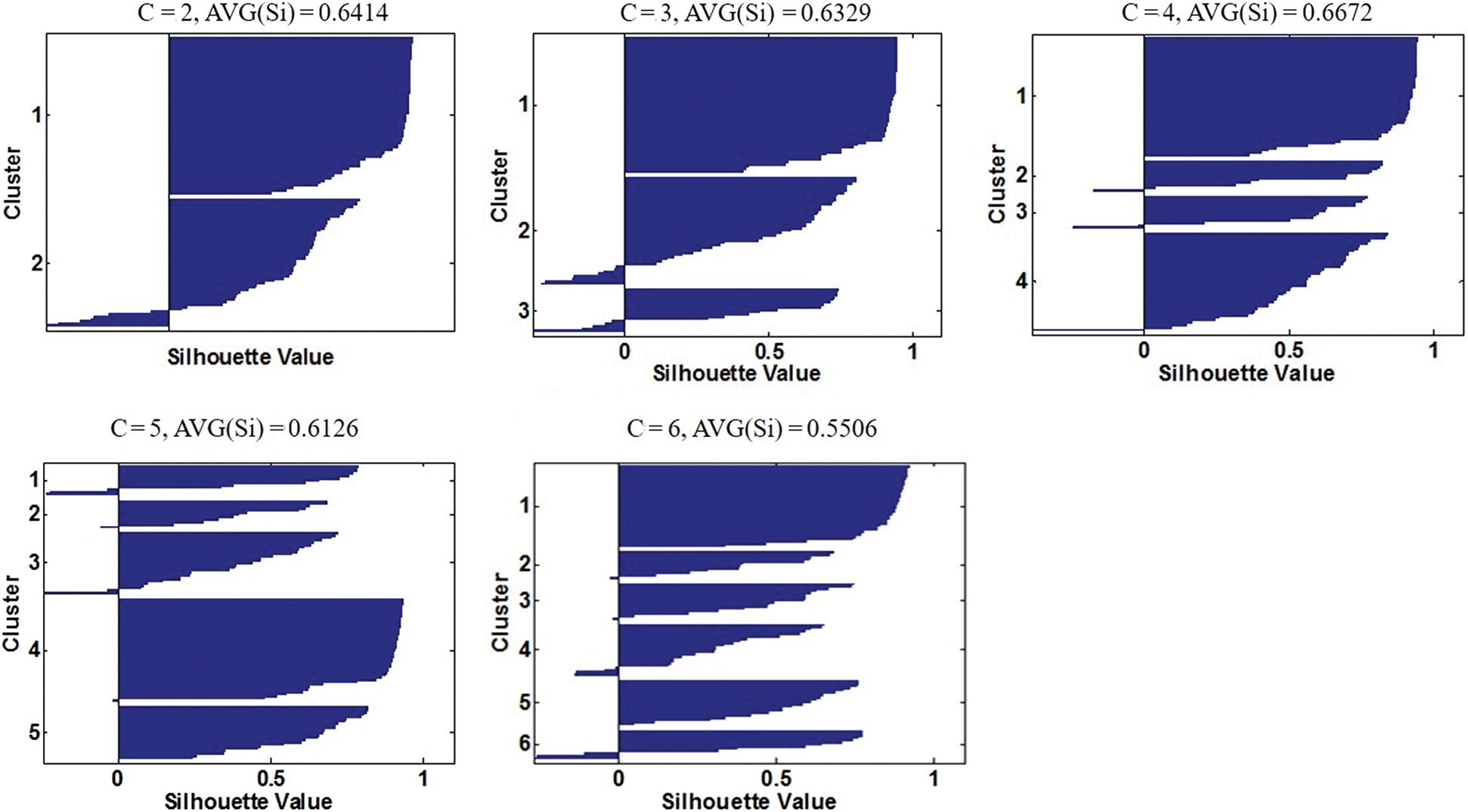
Figure 1: Silhouette graphics of different attempted cluster numbers (C). From left to right and top to down, the silhouette graph is displayed in an order of 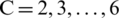, respectively. In each graph, the x-axis represents the silhouette values (Si) of (VAT, SAT) data, the y-axis represents the cluster number (C), and AVG(Si) denotes the average silhouette value of the current graph. The frequency that a graph is interrupted by zero or negative Si points indicates the number of separate clusters

The four clusters, representing four different fat distribution patterns, are shown in Fig. 2. The first cluster (C1), denoted by red triangles in the figure, consisted of the relatively healthy participants with normal VAT and SAT volumes, and the second cluster (C2), denoted by purple squares, was a group of the participants having moderately elevated VAT and SAT volumes. The third and fourth clusters (C3 and C4), indicated by blue diamonds (C3) and by green circles (C4), signified the unbalanced abdominal fat distributions with either significantly higher VAT or SAT. Out of 120 participants (66 men and 54 women), C1 had 22 female and 29 male participants; C2 included 26 women and 16 men with moderately elevated VAT and SAT; C3 contained six women and eight men whose SATs were significantly higher; and C4 comprised all 13 male participants who had considerably higher VATs.

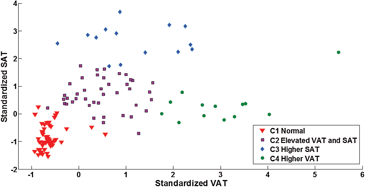
Figure 2: Final clustering results with the optimal cluster number () reflecting four categories of abdominal fat distribution. SAT (y-axis) and VAT (x-axis) values were standardized

The ANOVA test found that the SAT volume, the VAT volume, and the VAT/SAT ratio were significantly different (p < 0.05) between the four clusters of the fat distribution. The Games–Howell post-hoc analysis [38] revealed the following several points. In terms of the VAT volume, all pairs of the clusters, except the pair of C2 and C3, were significantly different. As for the SAT volume, all possible pairs of the clusters were significantly different. According to the VAT/SAT ratio, C4 was significantly different from the other three clusters. The box plots of the comparisons are shown in Fig. 3.

Figure 3: Box plots of the VAT, SAT and VAT/SAT ratio of the four fat distribution clusters (VAT: Visceral adipose tissue and SAT: Subcutaneous tissue)

3.2 Feature Selection

The three sets of obesity measurements (i.e., traditional, DXA and BSD sets) were scaled into [0,1] and compared via ANOVA. The differences in ethnicity in the traditional set and ASI in the BSD set among the four clusters were insignificant (p > 0.05). Therefore, these two measurements were excluded from the feature selection. All other measurements were retained as the inputs of the RBF-SVM classifier with the embedded mRMR, feature ranking and forward selection procedures. The feature selection procedures led to the following 13 features:

  1.  In the traditional set, WC, sex and BMI were the optimal features with a CV of 85%.

  2.  In the DXA set, Android FM, Gynoid FM and Trunk FM were the best features with a CV of 87.5%.

  3.  In the BSD set, CD, HipW, WaistW, HipV, WaistD, TorsoV, CW and CG6 were the elected features with a CV of 90%.

3.3 Fat Distribution Clusters and BSDs

Relationships between the fat distribution patterns and some of the BSDs were investigated further. Selective bar charts in Fig. 4 reveal the individuals in the same fat distribution cluster also possess similar body shapes. Fig. 4a shows that the thigh volumes of the participants with large SAT volumes (C3) were much higher than those with small SAT volumes. The 13 male participants in C4 had significantly higher values in VAT, as well as in CP and CSI (Figs. 4b and 4d). Meanwhile, the C4 participants had the lowest PSI and TVR values (Figs. 4c and 4e), indicating that less fats were distributed around their hips and thighs.

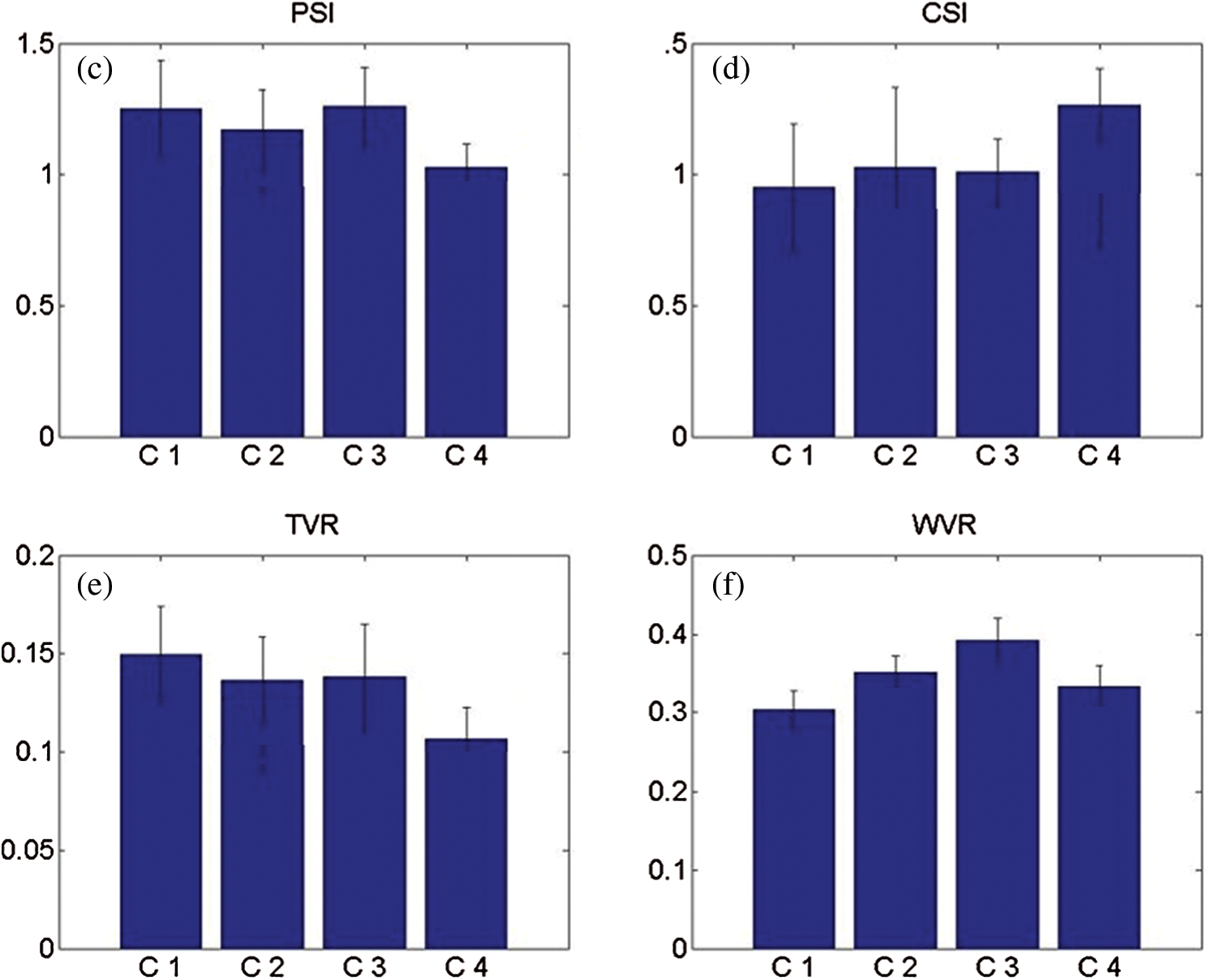
Figure 4: Bar charts of the body shape descriptors in the four fat distribution clusters. (a) ThighV (thigh volume), (b) CP (central protrusion), (c) PSI (pear shape index) (d) CSI (central shape index) (e) TVR (thigh volume ratio) and (f) WVR (waist volume ratio)

The participants with elevated VAT and SAT in C2 had slightly higher WVR values and lower TVR values than the lean participants in C1 (Figs. 4e and 4f), which indicated that those with high internal adiposity had more fat tissues around their waists and less fat tissues around their thighs. This finding was consistent with previous reports that lower extremity fat was associated favorably with glucose metabolism [39]. Moreover, the participants with lower level abdominal adiposity in C1 showed higher TVR values than the participants in the other three categories (Fig. 4e), suggesting that a large portion of the body fat tissue of a lean participant was located in the thighs. For the participants in C3 with higher SAT volumes, the ThighV and WVR values were much higher than those of the other participants (Figs. 4a and 4f). This result indicates that the fat accumulations of the individuals in C3 were mainly around the thighs and waists.

Fig. 5 is an example of 3D body images for each fat distribution cluster. Fig. 5a is a lean male participant in C1, Fig. 5b shows a shape-balanced male in C2 with moderately elevated VAT and SAT, Fig. 5c shows a high SAT male with a high fat accumulation around his waist and hip areas, and Fig. 5d shows a high VAT male in C4 with a prominent abdominal protrusion. Both Figs. 4 and 5 demonstrate associations between internal abdominal adiposity and external body shape characteristics.

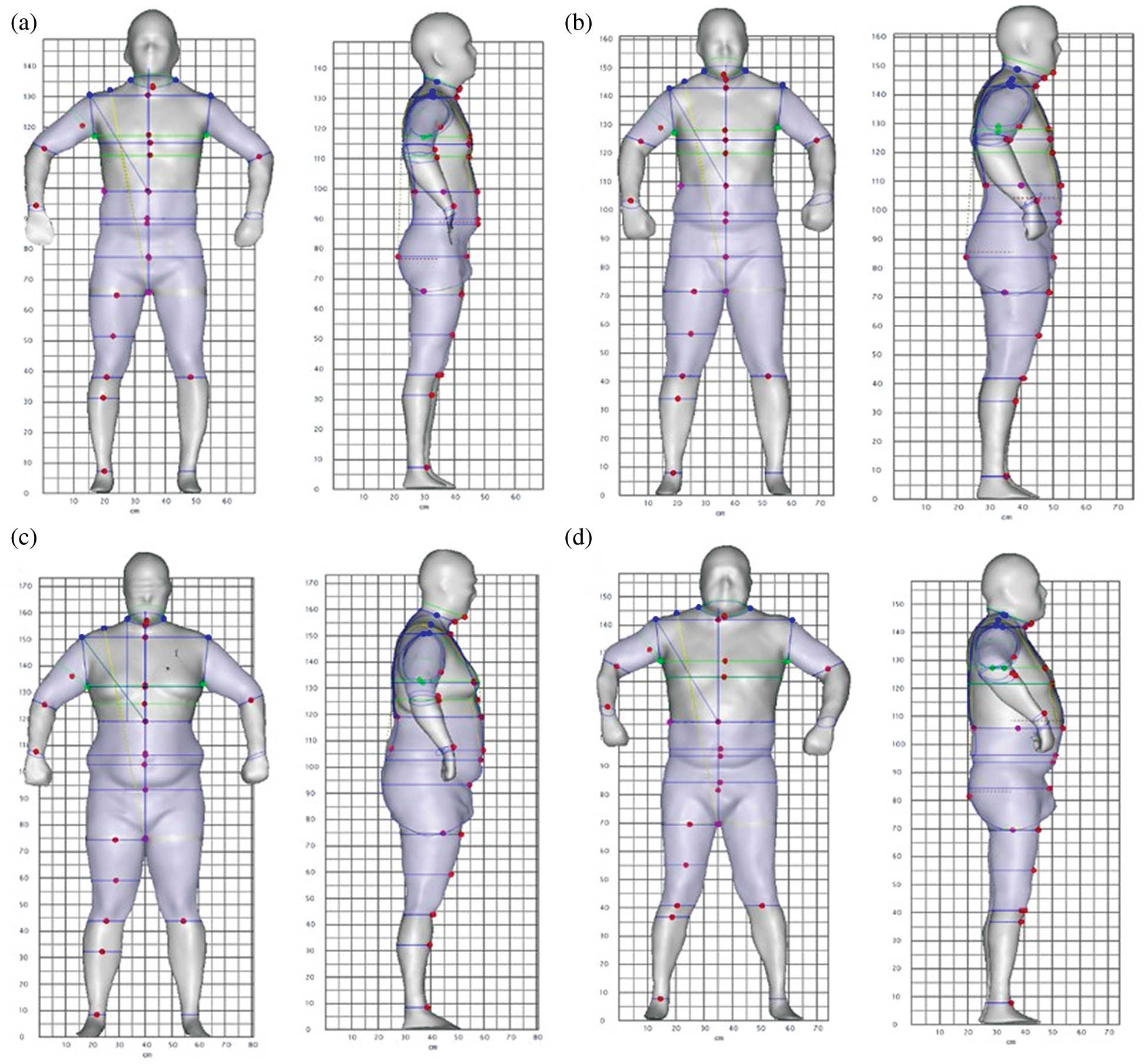
Figure 5: Examples of male participants in four categories of abdominal adiposity. (a) C1–-a participant with low VAT and SAT volumes, (b) C2–-a participant with moderately elevated VAT and SAT volumes, (c) C3–-a participant with significantly higher SAT volume and (d) C4–-a participant with significantly higher VAT volume

4  Discussion

In this study, a new categorization method was developed to explore the different patterns of abdominal fat distribution. The MRI sequences acquired from 120 participants with a wide range of BMIs and ages were used to calculate the VAT and SAT volumes that were the ground truth for the abdominal adiposity in the clustering and classification. Four clusters of abdominal adiposity were determined by the clustering analysis: (1) C1–participants with lower VAT and SAT volumes, (2) C2–-participants with moderately elevated VAT and SAT volumes, (3) C3–-participants with significantly higher SAT volumes and (4) C4–-participants with significantly higher VAT volumes. Note that the 13 participants grouped in C4 are all male. The finding about C4 is in agreement with previous studies that men tended to accumulate more visceral fats around the abdomen as compared to women [40].

The effectiveness of different obesity measurements for predicting the known fat distribution categories was tested via an optimized SVM classification scheme. A 3-stage feature selection method was utilized to search for the optimal subsets of the measurements that provide the highest classification accuracy with the least redundant information. Of the 120 participants, the sample numbers in the different fat distribution clusters were unequal: 51 in C1, 42 in C2, 14 in C3 and 13 in C4, respectively. Two classes, C1 and C2, comprised the majority of the participants. In general, an SVM classifier searches for the best hyperplane that can maximize the margin between classes for a low expected risk for future unknown samples [41]. However, the SVM classifier may lose its effectiveness and generalization ability when a highly unbalanced dataset is present. Therefore, unbalanced dataset should not be overlooked in the classification analysis.

Under-sampling and over-sampling techniques are the methods commonly used to randomly reduce samples from, or add samples to, specific classes in order to generate a more balanced dataset [42]. Because these two techniques may cause an inherent loss of valuable information or an addition of noise, a different technique was selected to manage the unbalanced sample size in this study by assigning different weights (wi) to the classes of different sizes [43]. Normally, a weight should be inversely proportional to the sample size. In this case, the sample size ratios for the four fat distribution clusters (C1/C2/C3/C4) were 4/4/1/1. Thus, the weights, w1 = 1, w2 = 1, w3 = 4 and w4 = 4, could be assigned to the four clusters.

The results of the classification analysis show that the 3D body shape descriptors provided the most accurate prediction for cluster labels of the abdominal fat distribution () among the three measurement sets. Thus, using the 3D body shape descriptors is a more accurate way to detect obesity as opposed to the traditional body measurements (). The DXA measurements () and demonstrates the potential to substitute for the traditional diagnostic methods. It should be noted that the body shape descriptors were obtained from a low-cost, portable 3D stereovision system that completes the image acquisition and quantitative measurements within a few seconds. In contrast, the traditional anthropometric measurements are more labor-intensive, time-consuming, inconvenient and subject to limited intra- and inter- reproducibility. The usage of DXA is an alternative method, but it is limited due to high cost and radiation exposure.

The BSDs that were not automatically selected in the feature selection scheme could be further examined by the SVM classifier after eliminating some selected descriptors. This would produce the three feature sets: (1) CD, WaistD, TorsoV, and CG6 (), (2) WasitD, CG6, WC, WaistV, CentralW, HipD and HipV (), and (3) PSI, WVR, TVR, and CW (). These three tested feature sets provided CV accuracies similar to the optimal feature set. The multiple sets of the body shape descriptors were able to predict the fat distribution clusters, and that the performance of the prediction was not heavily dependent on the selection of the descriptors.

A limitation of this study is the lack of metabolic risk factor data, such as blood pressure, blood lipids, glucose tolerance, and other biomarkers, for further association analysis with the BSDs. Future work should explore relationships between BSDs and metabolic risk factors. The sample size used for the natural clustering of abdominal adiposity also was limited. A more extended population size should be sampled in a future study to improve statistical power and eliminate potential sampling bias. Future research should also consider differences in fat distribution patterns among different demographic groups such as ethnicity, gender and age.

5  Conclusions

In this study, four clusters that discern distinctive abdominal fat distribution classes were identified: (1) Low adipose tissue, (2) Elevated VAT and SAT, (3) High VAT, and (4) High SAT. These classifications were based on the MRI visceral and subcutaneous fat data of 120 participants. Then the linkages of each of the clusters with the body shape descriptors (BSDs) of these participants were identified, as measured by our stereovision body imaging (SBI) system previously developed. An SVM classifier was created to predict the classes of internal body fat distributions (VAT/SAT) when the external BSDs of a person were measured by SBI. In addition to the paired MRI and SBI data, the traditional anthropometric and DXA data of the participants were collected and utilized to create the corresponding SVM classifiers to predict the clusters of abdominal VAT/SAT distributions. The accuracies of classifying the VAT/SAT clusters with the traditional anthropometric, DXA and BSD data were 85.0%, 87.5% and 90%, respectively. Thus, the BSDs appeared to be the most effective among the three sets of body measurements in predicting abdominal fat distributions.

Funding Statement: The author(s) received no specific funding for this study.

Conflicts of Interest: The authors declare that they have no conflicts of interest to report regarding the present study.

This work is licensed under a Creative Commons Attribution 4.0 International License, which permits unrestricted use, distribution, and reproduction in any medium, provided the original work is properly cited.