DOI: 10.32604/cmes.2021.012112
ARTICLE
A Novel Collaborative Filtering Algorithm and its Application for Recommendations in E-Commerce
1School of Design, Jiangnan University, Wuxi, 214122, China
2Department of Clothing Design and Engineering, Nantong University, Nantong, 226001, China
3Research Center for Intelligence Information Technology, Nantong University, Nantong, 226001, China
4School of Artificial Intelligence and Computer Science, Jiangnan University, Wuxi, 214122, China
5Management and Science University, Shah Alam, Selangor, 40100, Malaysia
*Corresponding Author: Juan Yang. Email: yjuan@ntu.edu.cn
Received: 03 June 2020; Accepted: 12 August 2020
Abstract: With the rapid development of the Internet, the amount of data recorded on the Internet has increased dramatically. It is becoming more and more urgent to effectively obtain the specific information we need from the vast ocean of data. In this study, we propose a novel collaborative filtering algorithm for generating recommendations in e-commerce. This study has two main innovations. First, we propose a mechanism that embeds temporal behavior information to find a neighbor set in which each neighbor has a very significant impact on the current user or item. Second, we propose a novel collaborative filtering algorithm by injecting the neighbor set into probability matrix factorization. We compared the proposed method with several state-of-the-art alternatives on real datasets. The experimental results show that our proposed method outperforms the prevailing approaches.
Keywords: Collaborative filtering; temporal behavior; probability matrix factorization
With the rapid development of the Internet, the amount of data recorded on the network has increased dramatically. It is becoming increasingly urgent to be able to effectively obtain the specific information we need from a vast ocean of data. Although traditional search engines can meet users’ retrieval requirements, they tend to return results with the same ranking to all users. Therefore, it is challenging to actively provide personalized services matching the interests of different users. Therefore, a recommendation system [1,2] is strongly desired. The recommendation system needs to learn users’ interests and behaviors after collecting and analyzing various data inputs by users so as to recommend tailored information and services. Because a recommendation system can effectively solve the information overload problem, it has received wide attention in academic and industrial fields.
Among all the recommendation methods, collaborative filtering [3,4] is the most commonly used algorithm. The core idea of collaborative filtering is to first analyze user interests based on user behavior records and then find neighbors from among the user group who have similar interests as the target. Then, by integrating all the evaluations from these neighbors, it finally generates an interest decision for the target user and thus recommends most related items. As collaborative filtering has no special requirements for the recommended items, it can handle objects that are difficult to describe by text, such as music and movies. Therefore, collaborative filtering has been widely used in recommendation systems. It has achieved significant performance and enabled great business benefits, especially to e-commerce. For example, according to statistics from VentureBeat, Amazon’s recommendation system provides them at least 35% of merchandise sales [5].
Although the collaborative filtering recommendation algorithm has many successful applications, several important issues need to be addressed. One significant issue is that traditional collaborative filtering often ignores the structural relationship between users or items. In the following, we only use users to represent “users (items).” Effectively making use of the relationships between users can enrich the information from a single user such that user interests can be identified more accurately. Based on this concept, many collaborative filtering algorithms have been developed that fully consider the user relationships for data mining. They have facilitated many valuable results. The process to obtain the relationships between users and then quantify the relationships has an important impact on the effectiveness of the collaborative filtering algorithms. The existing solutions mainly consist of two types: one makes use of the relationships existing in the explicit social network, and the other calculates the similarity between users through implicit label information to get the relationship between users. However, in practical applications, it is difficult to obtain sufficient information regarding social relationships or labels. Moreover, the above solutions are based on the vague assumption that the interaction between users is undirected, which is not reasonable in reality. For example, if user A highly appreciates user B, then the behavior of user B has a great impact on user A. However, the impact user A has on user B is not significant or even negligible.
In this study, to address the above issues, we propose a nearest neighbor modeling method based on temporal consumption behavior. Constructing a temporal-based consumption network helps identify the interactions between users. The contributions can be summarized as follows:
The proposed modeling strategy only requires the user’s consumption time rather than complicated information such as user labels and social relationships. The calculated influence is directed. The strategy can more accurately discover the interactions between users and identify the biggest impact on the current user from the neighbor set.
Based on the modeling strategy, a recommendation algorithm termed TemporalMF is developed, which uses the neighbor set for collaborative filtering recommendation based on probability matrix factorization.
We do extensive experiments on the Douban recommendation dataset. The experimental results show that by using social network information and label information, TemporalMF can predict the users’ actual scores more effectively and hence improve the accuracy of recommendations compared to traditional recommendation algorithms.
The remaining sections are arranged as follows. Section 2 briefly reviews related works about collaborative filtering. Section 3 describes the TemporalMF algorithm and its corresponding recommendation framework. In Section 4, some benchmarking algorithms are introduced for comparison. The last section concludes the study.
2.1 Traditional Collaborative Filtering Algorithms
Collaborative filtering makes use of the behaviors (scores, clicks, etc.) from similar users to predict the interest of the target user for a particular item. It then makes corresponding recommendations based on the predicted interest. Currently, popular collaboration filtering recommendation algorithms can mainly be divided into the neighborhood-based type and the model-based type.
Neighborhood-based collaborative filtering first calculates the similarity between users based on their historical information and then uses the evaluation of other items by neighbors with high similarity to the target user to predict the user’s preference for specific items. The preference degree of users is considered as the recommendation threshold. At present, neighbor-based collaborative filtering mainly includes the user-based type and the item-based type. The core of user-based collaborative filtering algorithms is to find similar users. Item-based algorithms mainly find similar items.
Different from nearest neighbor-based collaborative filtering, model-based collaborative filtering mainly trains a model through users’ rating data and then uses this model to predict the unknown variables [6]. At present, model-based collaborative filtering mainly consists of clustering models [7], probabilistic correlation models [8,9], latent factor models [10–12], and Bayesian hierarchy models [13,14]. Recently, in response to the requirements of big data processing, Mnih et al. [15] proposed a probabilistic matrix factorization (PMF) algorithm that uses a low-dimensional approximate matrix decomposition for generating a recommendation. In general, it assumes that the interest of each user is affected by only a few factors. In PMF, the user or item is mapped into a low-dimensional feature space, and the rating matrix is reconstructed through learning the user eigenvector from the user rating information. With the reconstructed low-dimensional matrix, the user’s rating of the item can be predicted, and corresponding recommendations can be derived. Owing to the low dimensions of the user and item eigenvectors, matrix factorization can be solved efficiently by gradient descent. Their experimental results show that PMF can effectively deal with large data and achieve relatively good accuracy. In order to reduce the negative effects caused by the parameter settings in PMF, Salakhutdinov et al. [16] proposed Bayesian probabilistic matrix factorization (BPMF). BPMF uses the Markov chain Monte Carlo algorithm for parameter estimation, which achieves better performance than PMF. In [17], the authors theoretically proved that PMF and probabilistic principal component analysis are consistent. Based on this justification, a non-linear PMF was proposed, which uses a Gaussian process to non-linearly expand PMF to obtain better performance.
Although traditional collaborative filtering algorithms can achieve satisfying recommendation performance, they often only take the scoring information into consideration and ignore temporal information and relationship information that is closely related to recommendations. Effective use of this information can further improve the accuracy of the recommendation. Therefore, many recommendation algorithms based on temporal information and relationship information have been proposed.
2.2 Temporal-Based Recommendation
A temporal-based recommendation takes temporal information into consideration. The derived model can learn the dynamic changes of data to optimize the recommendation. Koren [18] proposed TimeSVD++ in which time information is added to the user eigenvector to avoid interest drifting. Their experimental results indicated the advantages of TimeSVD++ . Xiong et al. [19] used time information as the third dimension and then used tensor decomposition to model dynamic changes. Chen et al. [20] dynamically assigned users to unused clusters to make further recommendations based on evolutionary co-clustering. Li et al. [21] argued that the interest of one user in a specific period will only focus on one or several aspects. Therefore, they proposed a cross-domain collaborative filtering framework. Experimental results showed that the framework can not only recommend effectively but also track the user interest drift direction. Ren et al. [22] argued that in existing recommendation systems, the user’s preference pattern and preference dynamic effect are both ignored. Therefore, they regularized the preference pattern into a sparse matrix and then used the corresponding subspace to gradually model personalized and global preference patterns.
Different from these related works, in this study we use temporal information to construct the structural relationship between users or items. Based on the structural relationship, the similarity is calculated and integrated into the probability matrix decomposition such that a new recommendation framework is generated.
2.3 Relationship-Based Collaborative Filtering
Traditional collaborative filtering algorithms generally assume that users or items are independent. So, they ignore the structural connection between users or items. Recommendation algorithms based on user or item relationship mining incorporate user or item relationships into existing collaborative filtering algorithms to enrich the information of a single user and hence improve the accuracy.
One of the core steps of the collaborative filtering algorithm based on relationship mining is to obtain the relationships between users. At present, the methods for obtaining user relationships are mainly divided into explicit and implicit types. In [23–25], the authors obtained the connections between users through explicit social network relationships. They added the users’ social relationship matrix to the original scoring matrix, which greatly improved the effectiveness of the algorithm. Jamali et al. [26] proposed a random walk model using a user trust relationship network. It finds similar items by performing random walks on social networks, thereby increasing the source of predicted scores for the target item and reducing the impact of data sparsity. It is difficult to obtain enough network relationships in the actual system. Zhou et al. [27] used label information to obtain the implicit relationship matrix for recommendations.
Considering that the above two types of relationship modeling methods are often affected by the difficulty of collecting large amounts of related data, in this study we mainly use the time sequence information of user consumption to mine the implicit relationships and integrate user or item relationships into the matrix factorization model. Finally, a collaborative filtering recommendation algorithm (termed as TemporalMF) based on time-sequential behavior is designed for recommendations.
3 Problem Definition and Probability Matrix Factorization
Suppose we have a recommendation system that contains Nu users denoted as  and contains Np items denoted as
  . The user-item rating matrix is denoted as
  , in which each element
  represents the rating of the i-th user for the j-th item. The collaborative filtering algorithm uses the probability matrix factorization model to learn the eigenvector of the user or item and then predicts the unknown rating based on this eigenvector.
Let  and
and  be the eigen matrices of the user and item, respectively. According to the above definitions, the conditional probability of the existing rating data is defined as follows:

where  represents the normal distribution with u and
  .
.  is a 0–1 function where if the i-th user rates the j-th item, it returns 1; otherwise, it returns 0.
  is a function to map x to [0, 1]. In this study,
  is adopted.
To avoid overfitting, the eigenvectors of the user and items are both assumed to follow the Gaussian prior distribution with u = 0 .
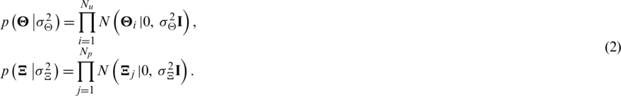
According to Bayesian inference theory, the posterior probability of  and
and  can be formulated as:
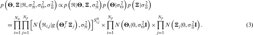
Fig. 1 shows a graph of probability matrix factorization [17]. According to (3), with the user-item rating matrix, it is easy to learn the corresponding eigenvector.

Figure 1: Graph of probabilistic matrix factorization
In this section, we give a detailed introduction of TemporalMF from three aspects. Firstly, we explain how to use the time sequence information of user consumption to mine the interactions between users or items so as to determine the neighbor set that has the greatest impact on users or items. Second, we explain how to successfully integrate this neighbor set into collaborative filtering based on probability matrix factorization. Lastly, detailed steps and computational complexity of TemporalMF are listed and analyzed.
4.1 Nearest Neighbor Selection Based on Time Sequence Behavior Modeling
In relationship-based matrix factorization, one of the core steps is to obtain a user or item relationship. Traditional collaborative filtering ignores the consumption time information. However, the time sequence information can provide some hidden patterns that can be used for mining relationships between uses and items. In order to discover these potential relationships, we first introduce a time sequence-based user consumption network, as shown in Fig. 2.

Figure 2: User consumption network
We use 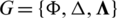 to represent the network shown in Fig. 2, where
  is the user set;
  represents the edge set; and
  represents the edge weight matrix. Digits in “( )” represent the number of items consumed by users. Within a given time period, if users
  and
and  consume the same item one after the other, then the weight
  of the edge
  increases by 1. By iterating all the products, we can update the edge weight matrix
  . Therefore, we can define the influence relationship weight as follows:

where  counts the number of same elements both contained in set A and set B .
  can be interpreted as the influence the i-th user has on the j-th user. For example, if the number of items that users
  and
and  consume is 100, then the influence
  imposes on
  is
is  . On the contrary, the influence
  imposes on
  is
is  . Therefore, we observe that the influence is directional, which is more reasonable than the undirected case.
Similarly, a time sequence-based item consumption network can be easily constructed. A toy example is shown in Fig. 3. Digits in “( )” now represent the number of users who consume the item; the weight  now represents the number of users who consume the items i and j one by one. Therefore, the influence relationship weight can be defined as:


Figure 3: Item consumption network
After mining the influence relationships between the corresponding users or items and finding the nearest neighbor set, we apply them to the matrix factorization model. As a result, the eigenvector of the user or item is affected by its nearest neighbors. In other words, similar users or items should have similar eigenvectors.
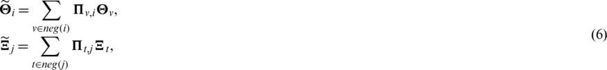
where  represents the neighbor set of i (user or item).
  and
and  represent the approximate eigenvectors, respectively. Unlike [6,8], our algorithm comprehensively considers the dual factors of the inner characteristics of users or items and the relationships. The eigenvector of each user or item not only follows the Gaussian prior distribution with
  to avoid overfitting but also needs to be similar to the user or item relationship eigenvector. As we consider the time sequence information, the influence relationship is clearer and more in line with the actual situation.
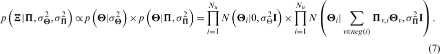

Similar to (3), with Bayesian inference theory, the posterior probability is deduced as follows:
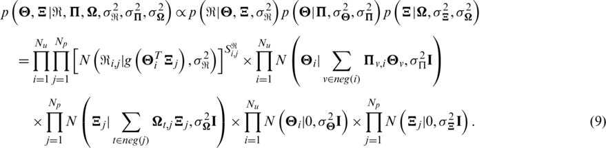
The probability map model of this model is shown in Fig. 4.

Figure 4: Framework of temporalMF recommendation
To facilitate the solution, the logarithmic of the posterior probability in (9) can be formulated as
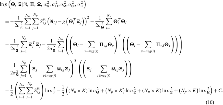
Maximizing this posterior probability is equivalent to minimizing the following objective function:
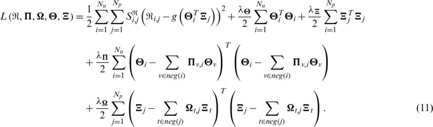
In (11),  . By employing the gradient descent method, we can obtain the eigenvector of each user or item.
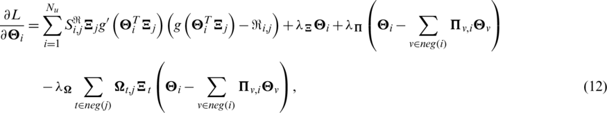
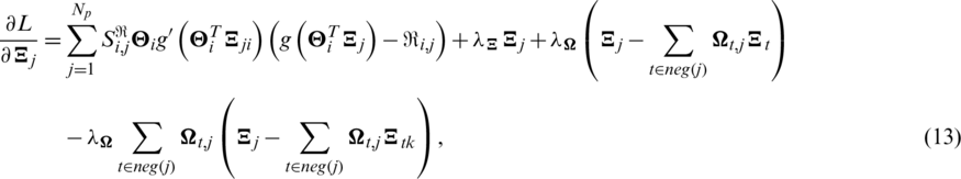
where  is the derivative of g(x). In this paper,
  .
.
4.3 Recommendation Algorithm Steps and Computational Complexity Analysis
The recommendation algorithm is divided into four steps:
Step 1: Data reading: The inputs contain the user’s rating information and rating time information.
Step 2: Neighbor set construction: According to the inputs, we build the consumption network of users and the consumption network of items. Then, we construct the nearest neighbor set.
Step 3: Probability matrix factorization: We apply the neighbor set to the probability matrix factorization model to learn the eigenvectors of users and items.
Step 4: Rating matrix reconstruction: Based on the eigenvectors of users and items, we reconstruct the rating matrix to obtain corresponding recommendations for users.
In our proposed algorithm, the steps that consume many CPU seconds are from two aspects. One is the consumption network construction and relationship mining. The other is the recommendation based on the obtained influence relationships. Let us take a user-based network as an example. Suppose that on average each item is consumed by  users. Sort each rating information according to the user’s rating time and then determine whether the edge weights involving these users have increased. According to this process, the complexity of creating a user consumption network for each item is
  , so the time complexity of establishing a user consumption network for all users is
  . Similarly, assuming that on average the number of items each user consumes is
  , then the time complexity of constructing the user consumption network of the item is
  . Therefore, the time complexity of constructing the user consumption network is
  . After we establish this network, we use the network to mine the influence relationships. Since each user consumes
  items on average, each user has
  edges in the network. Therefore, the time complexity of calculating the influence of each user on other users in turn and sorting is
  . Similarly, in the item-based consumption network, this time complexity is
  . According to the above analysis, the total time complexity of the first aspect is
  .
.
For the second aspect, according to the analysis in [6], the time complexity of the gradient computation is  , where l represents the number of neighbors that affect users. The establishment of the network only needs to traverse the rating information in turn, without iteration. Besides,
  and
and  are often relatively small, so the total time complexity of the model is not high and it can be effectively used for big data processing.
Fig. 4 illustrates the specific process of the algorithm, in which each step is detailed introduced.
In this section, we first briefly introduce the datasets used in our experiments and then describe the evaluation criteria and comparison algorithms. Finally, we give the comparative experimental results of our proposed model and comparison algorithms.
In order to compare the impact of different information and relationships on the recommendation results, the experimental datasets should contain rating information, label information, and user social relationships. To this end, we collected such data from the Douban website as our experimental datasets. Douban is a very popular website for evaluating, discussing, and recommending movies, books, and music. The site can provide users with ratings, discussions, and recommendations. It has the largest data of books, music, and movies in China and is one of the largest online communities in China. On the website, each user can rate books, music, or movies within the range [1,5]. In addition, Douban also provides a Facebook-like social relationship service, which allows users to discover their friends via e-mail addresses. In summary, the Douban data is suitable for our experimental studies.
The dataset we used in this study is listed in Tab. 1, which contains two groups of data. One group is the user’s rating information on the book, the user’s social relationship, and tag information. The other group is the user’s rating information on the movie and other corresponding information.

We adopt RMSE [28–30] as the evaluation criteria in this study:

where  represents the predictive vector, and
  represents the ground-truth vector.
5.3 Comparison Algorithms and Parameter Settings
We selected four methods as comparison algorithms. They are PMF, BPTF, SocialMF, and TagMF. In our experiments, we referred to the original references to set their corresponding parameters.
5.4 Experimental Results and Analysis
In this section, we report our experiments from three aspects, namely the performance with different dimensions of the eigenvector, the computational complexity, and the robustness analysis.
First, we set the dimension of the eigenvector K to 5, 10, and 20, respectively. Tab. 2 shows the RMSEs of all algorithms with different K. We observe that our proposed algorithm achieves the best performance with each K. We obtained the following important results.
1. With the increase of K, the accuracy of the algorithm improved slightly. However, it should be noted that the increase of K will also increase the time complexity of the model to a certain extent.
2. Compared with PMF, the performance of BPTF, TagMF, SocialMF, and the proposed algorithm is significantly improved, which indicates that the relationship between temporal information and users (items) plays a greater role in improving the accuracy of traditional collaborative filtering algorithms.
3. Compared with SocialMF, the performance of BPTF is improved, which is mainly caused by the sparse social relationships displayed in SocialMF. Compared with TagMF and TemporalMF, the results of BPTF are slightly worse.
4. Compared with TagMF and our method, SocialMF performs a little worse, which is mainly because SocialMF does not consider the relationships between items. In addition, SocialMF does not consider the direction of the relationship between friends.
5. Compared with TagMF, the proposed algorithm outperforms substantially, which indicates that the impact relationship proposed in this article can effectively improve the accuracy of the algorithm. In addition, because the proposed algorithm only requires simple time information, from the perspective of information acquisition and applicable scope, the proposed algorithm also has an advantage.
Table 2: RMSEs of all algorithms with different K

The experimental results show that the proposed algorithm performs the best compared to traditional PMFs, which fully illustrates the rationality and effectiveness of the impact relationship proposed in this paper. Compared to SocialMF, TagMF, and BPTF, although the improvement is not very significant, in actual recommendation systems, the social network relationships or tag information required by SocialMF and TagMF are often difficult to obtain or extremely sparse, whereas the proposed algorithm only requires time information that is very easy to obtain. Therefore, the proposed algorithm can be widely used in many practical applications.
Tab. 3 gives the CPU seconds of each iteration for all algorithms under the environment of Intel Core i3 CPU, 2.67 GHZ, Windows 7 system, 8 GB memory.
Table 3: CPU seconds of each iteration all algorithms consume
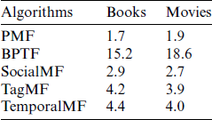
We see that the consumed CPU seconds of BPTF are much higher than other algorithms. This is mainly because BPTF consumes too many CPU seconds for Markov Monte Carlo training, so the computational complexity of BPTF is high. In addition, Tab. 3 also indicates that the more relationships there are, the higher is the computational complexity. In general, the CPU seconds taken by TemporalMF are acceptable. For PMF and BPTF, the CPU seconds on books are less than that on movies. The rest of the algorithms are the opposite. This is mainly because PMF and BPTF do not consider neighbor relationships, so their computational complexity is only related to the amount of rating data in the training set. The rating data for books is scarce compared to the rating data for movies Tab. 1, so books requires fewer CPU seconds. The rest of the algorithms take the neighbor relationships into account. Since the books dataset contains more users and items than the movies dataset, algorithms consume more CPU seconds for books.
In TemporalMF, the parameter  can measure the degree to which users or items are affected by their relationship information. The larger the
  , the greater is the effect that the user or item has on the algorithm relationships. In order to reduce complexity in this experiment, we set
 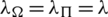 . The values of
  are set to 0.1, 0.5, 1, 5, 10, and 20, respectively. In addition, we set K to 5. Fig. 5 shows the performance of TemporalMF with different
  on books and movies. According to the results, we can see that parameter
  has a greater impact on TemporalMF. With the increase of
  , the performance of TemporalMF improves. This fully illustrates the reliability of the relationships obtained by the temporal information in this article and the benefit of the introduction of the relationships to the algorithm. We found when
  increases to 20, its impact on TemporalMF starts to decline. This is mainly due to the over-fitting of the algorithm caused by
  being too large, which leads to a decrease in accuracy.

Figure 5: Performance of TemporalMF with different 
In order to compare the effects of the algorithms under different sparsity conditions, we use the number of user ratings as a basis for dividing the users in the training set into four groups, namely [0:10], [10:100], [100, 500], and [500, inf]. Fig. 6 illustrates the proportion of each group of users in the two sets of data.

Figure 6: Distribution of different types of users
After dividing the data accordingly, we use the training set to learn the corresponding model and then calculate RMSE for the four groups of users on the test set. We observe that:
In the case of extremely sparse data (the number of scores is less than 10), the improvement effect of TemporalMF is not obvious, and it is worse than SocialMF and TagMF that introduce additional information. This is mainly because the sparse data will cause the network graph created by TemporalMF to be extremely sparse, which affects its accuracy. BPTF introduces parameter training methods, so it performs better than TemporalMF. However, TemporalMF is still better than traditional PMF.
When user rating data increases, TemporalMF is better than TagMF, SocialMF, and BPTF, which further proves that the impact relationships introduced in this article can effectively improve the accuracy of the recommendation system.
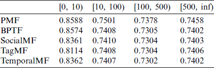
It can also be seen from Tabs. 4 and 5 that no matter whether it is TemporalMF or other algorithms, the RMSE results do not continue to decrease with the increase in the number of ratings. When the number of ratings is 500 and higher, the effect of the algorithm begins to decline. This is mainly because when the number of scores is small, the sparseness of the data affects the performance of the algorithm. At this time, the model is prone to over-fitting. The training accuracy is good, but the accuracy on the test samples is poor. As the number of scores increases, the data gradually becomes denser, thereby alleviating the impact of sparse data, and the effect of the algorithm gradually becomes better. When the scored training samples pass After more, the user’s interest will diverge. This will cause the model to fail to learn the user’s feature preferences, which will affect the accuracy of the model. Therefore, controlling the number of samples has a certain impact on the prediction effect of the model. It can be seen from Tabs. 4 and 5 that for the dataset of this article, when the number of user samples is (100–500), the algorithm works best.
Table 4: RMSEs of all algorithms with different number of user scores (book)
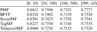
Table 5: RMSEs of all algorithms with different number of user scores (movie)
This study uses temporal information to establish a user (item) consumption network. Through this network, the user (item) potential interaction relationship and the nearest neighbor set are found. Then, they are incorporated into a matrix filtering-based collaborative filtering recommendation algorithm. As a result, the accuracy of score prediction is improved. Since the consumption time information is easier to obtain compared to social network information and tag information, the application of collaborative filtering recommendation algorithms based on temporal behavior is more widely possible. Experiments on Douban recommendation datasets show that this method has strengths compared with traditional recommendation algorithms. In future work, we will further study the challenges in this method arising from solving the problem of a sparse consumption network and the cold start of users and items. In addition, the relationship acquisition method we propose is not limited to the probability matrix decomposition algorithm. We can also consider applying this technique to other matrix factorization methods. In future work, we will also study the use of this method to further improve the recommendation predictions.
Funding Statement: This work was supported by the National Natural Science Foundation of China under Grant Nos. 81873915, 61702225 and 61806026, Ministry of Science and Technology Key Research and Development Program of China under Grant No. 2018YFC0116902, by the Natural Science Foundation of Jiangsu Province under Grant No. BK20180956, by the 2018 Six Talent Peaks Project of Jiangsu Province under Grant No. XYDXX-127, by the Science and Technology demonstration project of social development of Wuxi under Grant WX18IVJN002, by the Philosophy and Social Science Foundation of Jiangsu Province (18YSC009).
Conflicts of Interest: The authors declare that they have no conflicts of interest to report regarding the present study.
1. Xu, X., Zhou, J., Liu, Y., Xu, Z., Zhao, X. (2015). Taxi-RS: Taxi-hunting recommendation system based on taxi GPS data. IEEE Transactions on Intelligent Transportation Systems, 16(4), 1716–1727. DOI 10.1109/TITS.2014.2371815. [Google Scholar] [CrossRef]
2. Baral, R., Iyengar, S. S., Zhu, X., Li, T., Sniatala, P. (2019). HiRecS: A hierarchical contextual location recommendation system. IEEE Transactions on Computational Social Systems, 6(5), 1020–1037. DOI 10.1109/TCSS.2019.2938239. [Google Scholar] [CrossRef]
3. Yang, B., Lei, Y., Liu, J., Li, W. (2016). Social collaborative filtering by trust. IEEE Transactions on Pattern Analysis and Machine Intelligence, 39(8), 1633–1647. DOI 10.1109/TPAMI.2016.2605085. [Google Scholar] [CrossRef]
4. Hu, Y., Peng, Q., Hu, X., Yang, R. (2014). Time aware and data sparsity tolerant web service recommendation based on improved collaborative filtering. IEEE Transactions on Services Computing, 8(5), 782–794. DOI 10.1109/TSC.2014.2381611. [Google Scholar] [CrossRef]
5. Liu, J., Zhou, T., Wang, B. (2009). Research progress of personalized recommendation system. Progress in Natural Science, 19(1), 1–15. DOI 10.1016/j.pnsc.2008.06.004. [Google Scholar] [CrossRef]
6. Yang, H., Ling, G., Su, Y., Lyu, M. R., King, I. (2015). Boosting response aware model-based collaborative filtering. IEEE Transactions on Knowledge and Data Engineering, 27(8), 2064–2077. DOI 10.1109/TKDE.2015.2405556. [Google Scholar] [CrossRef]
7. Zhang, Y., Chung, F. L., Wang, S. (2020). Clustering by transmission learning from data density to label manifold with statistical diffusion. Knowledge-Based Systems, 193(6), 1–14. DOI 10.1016/j.knosys.2019.105330. [Google Scholar] [CrossRef]
8. John, D. J., Fetrow, J. S., Norris, J. L. (2010). Continuous cotemporal probabilistic modeling of systems biology networks from sparse data. IEEE/ACM Transactions on Computational Biology and Bioinformatics, 8(5), 1208–1222. DOI 10.1109/TCBB.2010.95. [Google Scholar] [CrossRef]
9. He, Z., Wu, J., Li, T. (2014). Label correlation mixture model: A supervised generative approach to multilabel spoken document categorization. IEEE Transactions on Emerging Topics in Computing, 3(2), 235–245. DOI 10.1109/TETC.2014.2377559. [Google Scholar] [CrossRef]
10. Ge, Z. (2015). Supervised latent factor analysis for process data regression modeling and soft sensor application. IEEE Transactions on Control Systems Technology, 24(3), 1004–1011. DOI 10.1109/TCST.2015.2473817. [Google Scholar] [CrossRef]
11. López-Lopera, A. F., Alvarez, M. A. (2017). Switched latent force models for reverse-engineering transcriptional regulation in gene expression data. IEEE/ACM Transactions on Computational Biology and Bioinformatics, 16(1), 322–335. DOI 10.1109/TCBB.2017.2764908. [Google Scholar] [CrossRef]
12. Luo, X., Zhou, M., Xia, Y., Zhu, Q., Ammari, A. C. et al. (2015). Generating highly accurate predictions for missing QoS data via aggregating nonnegative latent factor models. IEEE Transactions on Neural Networks and Learning Systems, 27(3), 524–537. DOI 10.1109/TNNLS.2015.2412037. [Google Scholar] [CrossRef]
13. Käser, T., Klingler, S., Schwing, A. G., Gross, M. (2017). Dynamic Bayesian networks for student modeling. IEEE Transactions on Learning Technologies, 10(4), 450–462. DOI 10.1109/TLT.2017.2689017. [Google Scholar] [CrossRef]
14. Chien, J. T. (2017). Bayesian nonparametric learning for hierarchical and sparse topics. IEEE/ACM Transactions on Audio, Speech, and Language Processing, 26(2), 422–435. DOI DOI 10.1109/TASLP.2017.2779862. [Google Scholar] [CrossRef]
15. Mnih, A., Salakhutdinov, R. R. (2008). Probabilistic matrix factorization. Advances in Neural Information Processing Systems, pp. 1257–1264, Canada. [Google Scholar]
16. Salakhutdinov, R., Mnih, A. (2008). Bayesian probabilistic matrix factorization using Markov chain Monte Carlo. Proceedings of the 25th International Conference on Machine Learning, pp. 880–887, Helsinki, Finland. [Google Scholar]
17. Lawrence, N. D., Urtasun, R. (2009). Non-linear matrix factorization with Gaussian processes. Proceedings of the 26th Annual International Conference on Machine Learning, pp. 601–608, Canada. [Google Scholar]
18. Koren, Y. (2009). Collaborative filtering with temporal dynamics. Proceedings of the 15th ACM SIGKDD International Conference on Knowledge Discovery and Data Mining, pp. 447–456, Paris, France. [Google Scholar]
19. Xiong, L., Chen, X., Huang, T. K., Schneider, J., Carbonell, J. G. (2010). Temporal collaborative filtering with Bayesian probabilistic tensor factorization. Proceedings of the 2010 SIAM International Conference on Data Mining, pp. 211–222, Columbus, Ohio, USA. Society for Industrial and Applied Mathematics. [Google Scholar]
20. Chen, J., Wei, L., Zhang, L. (2018). Dynamic evolutionary clustering approach based on time weight and latent attributes for collaborative filtering recommendation. Chaos, Solitons & Fractals, 114(1), 8–18. DOI 10.1016/j.chaos.2018.06.011. [Google Scholar] [CrossRef]
21. Li, B., Zhu, X., Li, R., Zhang, C., Xue, X. et al. (2011). Cross-domain collaborative filtering over time. Proceedings of the Twenty-Second International Joint Conference on Artificial Intelligence, pp. 2293–2298, Freiburg, Germany. [Google Scholar]
22. Ren, Y., Zhu, T., Li, G., Zhou, W. (2013). Top-N recommendations by learning user preference dynamics. Pacific-Asia Conference on Knowledge Discovery and Data Mining, pp. 390–401, Berlin, Heidelberg: Springer. [Google Scholar]
23. Ma, H., Yang, H., Lyu, M. R., King, I. (2008). Sorec: Social recommendation using probabilistic matrix factorization. Proceedings of the 17th ACM Conference on Information and Knowledge Management, pp. 931–940, Singapore. [Google Scholar]
24. Ma, H., King, I., Lyu, M. R. (2009). Learning to recommend with social trust ensemble. Proceedings of the 32nd International ACM SIGIR Conference on Research and Development in Information Retrieval, pp. 203–210, Boston, MA, USA. [Google Scholar]
25. Guo, L., Ma, J., Chen, Z., Jiang, H. (2012). Learning to recommend with social relation ensemble. Proceedings of the 21st ACM International Conference on Information and Knowledge Management, pp. 2599–2602, Maui Hawaii, USA. [Google Scholar]
26. Jamali, M., Ester, M. (2009). Trustwalker: A random walk model for combining trust-based and item-based recommendation. Proceedings of the 15th ACM SIGKDD International Conference on Knowledge Discovery and Data Mining, pp. 397–406, Paris, France. [Google Scholar]
27. Zhou, T. C., Ma, H., Lyu, M. R., King, I. (2010). UserRec: A user recommendation framework in social tagging systems. Association for the Advancement of Artificial Intelligence, pp. 11–15, Atlanta, Georgia. [Google Scholar]
28. Zhang, Y., Ishibuchi, H., Wang, S. (2017). Deep Takagi-Sugeno–Kang fuzzy classifier with shared linguistic fuzzy rules. IEEE Transactions on Fuzzy Systems, 26(3), 1535–1549. DOI 10.1109/TFUZZ.2017.2729507. [Google Scholar] [CrossRef]
29. Zhang, Y., Chung, F. L., Wang, S. (2018). A multiview and multiexemplar fuzzy clustering approach: Theoretical analysis and experimental studies. IEEE Transactions on Fuzzy Systems, 27(8), 1543–1557. DOI 10.1109/TFUZZ.2018.2883022. [Google Scholar] [CrossRef]
30. Zhang, Y., Chung, F. L., Wang, S. (2017). Fast reduced set-based exemplar finding and cluster assignment. IEEE Transactions on Systems, Man, and Cybernetics: Systems, 49(5), 917–931. DOI 10.1109/TSMC.2017.2689789. [Google Scholar] [CrossRef]
 | This work is licensed under a Creative Commons Attribution 4.0 International License, which permits unrestricted use, distribution, and reproduction in any medium, provided the original work is properly cited. |