Computer Modeling in Engineering & Sciences

DOI: 10.32604/cmes.2021.014580

ARTICLE

Bioprosthetic Valve Size Selection to Optimize Aortic Valve Replacement Surgical Outcome: A Fluid-Structure Interaction Modeling Study

Caili Li1, Dalin Tang2,3,*, Jing Yao4,*, Christopher Baird5, Haoliang Sun6, Chanjuan Gong7, Luyao Ma6, Yanjuan Zhang4, Liang Wang2, Han Yu2, Chun Yang8 and Yongfeng Shao6

1School of Mathematics, Southeast University, Nanjing, 210096, China
2School of Biological Science & Medical Engineering, Southeast University, Nanjing, 210096, China
3Mathematical Sciences Department, Worcester Polytechnic Institute, Worcester, MA 01609, USA
4Department of Cardiology, First Affiliated Hospital of Nanjing Medical University, Nanjing, 210029, China
5Department of Cardiac Surgery, Boston Children’s Hospital, Harvard Medical School, Boston, MA 02115, USA
6Department of Cardiovascular Surgery, First Affiliated Hospital of Nanjing Medical University, Nanjing, 210029, China
7Department of Anesthesiology, First Affiliated Hospital of Nanjing Medical University, Nanjing, 210029, China
8China Information Technology Designing & Consulting Institute Co., Ltd., Beijing, 100048, China
*Corresponding Authors: Dalin Tang. Southeast University. Email: dtang@wpi.edu; Jing Yao. Email: echoluyao@163.com
Received: 10 October 2020; Accepted: 23 December 2020

1  Introduction

Aortic valve disease affects more than 60 million people worldwide, with prevalence growing resulting from an ageing population [1]. Aortic valve replacement (AVR) remains a major treatment option for the patients with severe aortic valve disease [1,2]. More than 200,000 surgical aortic valve replacements are performed yearly worldwide [3]. Bioprosthetic valve is the most popular choice for AVR, with a proportion of over 85% [1]. Clinical outcome of AVR is strongly dependent on appropriate choice of prosthesis size and replacement technique, which is currently primarily dependent on the experience and skill of the surgeon [4,5]. Patients receiving AVR are at risk of prosthesis–patient mismatch (PPM) if a prosthetic valve with wrong size is implanted [6]. Results from clinical studies showed that PPM after AVR is associated not only with incidence of operative mortality and late cardiac events, but also with negative effects on left ventricular (LV) systolic function recovery, hemodynamics, quality of life, and bioprosthetic valve durability [7–9]. Fortunately, studies have shown that aortic root enlargement may be an important option adjunct to AVR to prevent or mitigate PPM. Yu et al. [6] suggested that adjunctive aortic root enlargement during surgical AVR may be a safe strategy to help facilitate the implantation of larger valve prostheses in selected patients.

We hypothesize that properly selected bioprosthetic valve with size larger than that recommended by current AVR guidelines may lead to better hemodynamics and cardiac function post AVR surgeries. However, due to high cost and risk involved in AVR surgery, it is not practical to test the hypothesis directly on patients. It is desirable to use computer-aided simulations to test the feasibility of the hypothesis before actual patient studies could be performed.

Recent advances in computational modeling techniques have made it possible for computational models to be constructed and used to simulate innovative high-risk surgical procedures and evaluate the impact of valve size on AVR surgical outcome. Previous numerical simulation of valve dynamics mainly focused on three categories: Structure mechanical analysis, computational fluid dynamics and fluid-structure interaction (FSI) modeling. Structure mechanical analysis mainly focuses on the dynamics of the leaflets, where a constant pressure value or a time-varying pressure was applied to the leaflets, ignoring the interaction between leaflets and blood flow [2,4,5,10–13]. For computational fluid dynamics simulation, only flow behaviors of blood flow were considered while the valve leaflets were fixed in the fully or partially open positions [14,15]. Deformation of the valve structure in the valve open-close process was ignored. Due to the limitations of structural mechanics analysis and computational fluid dynamics methods, more and more studies have focused on FSI modeling to simulate the interaction between valves and blood flow, which can describe more realistically the dynamic flow field of the entire cardiac cycle [16,17]. Boundary-fitted or non-boundary-fitted flow meshes are two available FSI techniques [16]. The arbitrary Lagrangian–Eulerian (ALE) method is a boundary fitted method, which synchronizes fluid and structural grid movement and achieves a noncompromised accuracy by satisfying the kinematic relation at the interface [16]. ALE is better suited to study prosthetic valve hemodynamics since the variables are calculated directly on the interface [16]. Several groups used ALE-FSI to study native or diseased or bioprosthetic aortic valve deformations [16,18–20]. Gharaie et al. [20] studied nonlinear deformation of polymeric aortic valves using an ALE-based Two-Way FSI model that was validated by in vitro benchtop testing. Ghosh et al. [16] implemented an ALE-FSI to compare the hemodynamic and mechanical behavior of polymeric transcatheter AVR and surgical AVR valves. Their results showed transcatheter AVR had larger opening area and higher flow rate than that from the surgical AVR. A comprehensive review of FSI models and simulation methods for aortic valves can be found from Marom et al. [21]. Zakerzadeh et al. [2] provided a review of bioprosthetic valve computational methods, with a focus on AVR. One-Way and fully-coupled Two-Way are two strategies for FSI coupling between the structure and fluid domains [22]. In a One-Way FSI study, fluid and structural governing equations were solved in series, where the solution of one domain was used as a boundary or initial condition in the second domain [22–24]. In a fully-coupled Two-Way FSI study, governing equations for the two domains are solved in parallel, and the solutions at each iteration for the fluid and structural domains must agree and reach convergence together [22,23]. Two-Way FSI has become the modeling standard for the study of cardiac valve dynamics [22]. Mao et al. [25] combined smoothed particle hydrodynamics and nonlinear finite element method to develop a transcatheter aortic valve full-coupled FSI model based on ideal geometry. Comparing the FSI model with smoothed particle hydrodynamics to the FSI model using only finite elements, they demonstrated that the two models had substantial differences in leaflet kinematics, and that the FSI model could capture the realistic leaflet dynamic deformation. Subsequently, they used the same method to introduce FSI models of the LV with mitral valve and aortic valve. By comparing with the LV model without valves, they revealed that the flow field of the two models had substantial differences and FSI models with valve dynamics should be used for ventricle flow and biomechanics investigations [26]. FSI aortic valve models have been used to study both normal [27,28] and diseased valves [29,30] and to evaluate bioprosthetic valves [16], but ALE based Two-Way FSI models to explore the effect of valve size on AVR are still lacking in the current literature.

In this study, ALE based Two-Way FSI models of aortic root were introduced to investigate the effect of valve size on hemodynamics of the implanted bioprosthetic valve and seek optimal outcome post AVR surgeries. Leaflets were described by nonlinear anisotropic constitutive laws, and we explored AVR optimize strategies by simulating entire cardiac cycle for different bioprosthetic valve sizes.

2  Valve Geometry, Patient Data, FSI Modeling, and Benchmark for Valve Optimization

2.1 3D Aortic Root Geometry Construction

The aortic root geometry included valvular leaflets, sinuses, interleaflet triangles and annulus. The aortic root model with 4 different sizes of bioprosthetic valves (19 (No. 19), 21 (No. 21), 23 (No. 23) and 25 mm (No. 25)) were constructed. Fig. 1 shows the geometric reconstruction process of aortic root based on well-accepted analytic models. Details of the valve model geometry reconstruction procedure was described in [31]. Model parameters for the four aortic root geometries under zero-load are shown in Tab. 1.

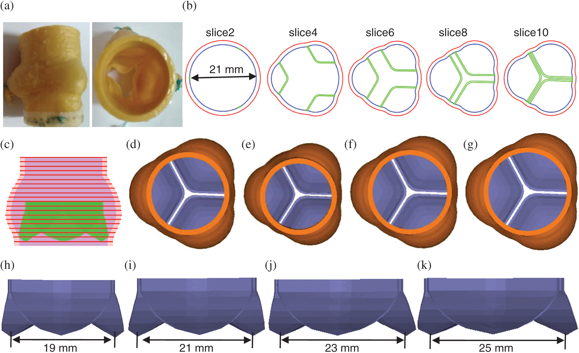
Figure 1: The aortic root three dimensional (3D) geometric reconstruction process. (a) A sample commercial aortic root bioprosthesis [31]. (b) Cross-section plots of aortic root slices at different heights. (c) Stacked contours showing leaflets. (d) Aortic root model with No. 21 valve. (e) Aortic root model with No. 19 valve. (f) Aortic root model with No. 23 valve. (g) Aortic root model with No. 25 valve. (h) No. 19 aortic valve. (i) No. 21 aortic valve. (j) No. 23 aortic valve. (k)No.25 aortic valve

Table 1: Model parameters for aortic root geometry with different valve sizes

2.2 Patient Data

Left ventricle outflow track (LVOT) flow data from one patient was collected and used as model flow conditions for our valve models (Fig. 2). The patient (m, age: 69), with body surface area was 1.9 cm2/m2, was recruited to participate in this study at the First Affiliated Hospital of Nanjing Medical University with written consent obtained. The study was approved by institutional review board at the First Affiliated Hospital of Nanjing Medical University. An AVR with bioprosthetic valve was performed for the patient following current AVR surgical guidelines. Fig. 3 shows the main steps of AVR surgery with aortic root enlargement procedure. Standard echocardiograms were obtained using an ultrasound machine (EPIQ 7C, Philips Mechanical Systems) with an X7 Transesophageal Echocardiography probe. LVOT diameter was measured from the middle esophagus LV outflow long axis view in mid-systole parallel to the valve plane and immediately adjacent to the aortic leaflet insertion into the annulus. Pulse Doppler-echo data were analyzed using QLAB software (Philips Mechanical Systems) by an independent observer unaware of the invasive data (Fig. 2a). The Pulse Doppler LVOT velocity curves were traced and the average systolic velocity profile was obtained for modeling use (see Fig. 2a).

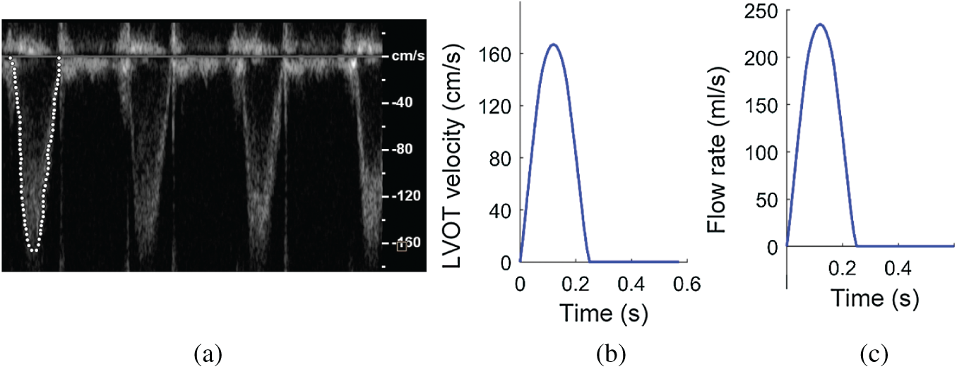
Figure 2: Blood flow velocity and flow rate of LVOT obtained from a patient. (a) LVOT velocity profile recorded by pulse Doppler-echo. (b) Imposed blood velocity profile at inlet (centerline velocity). (c) Flow rate curve calculated using the center line velocity profile given in (b) and used for all valve models

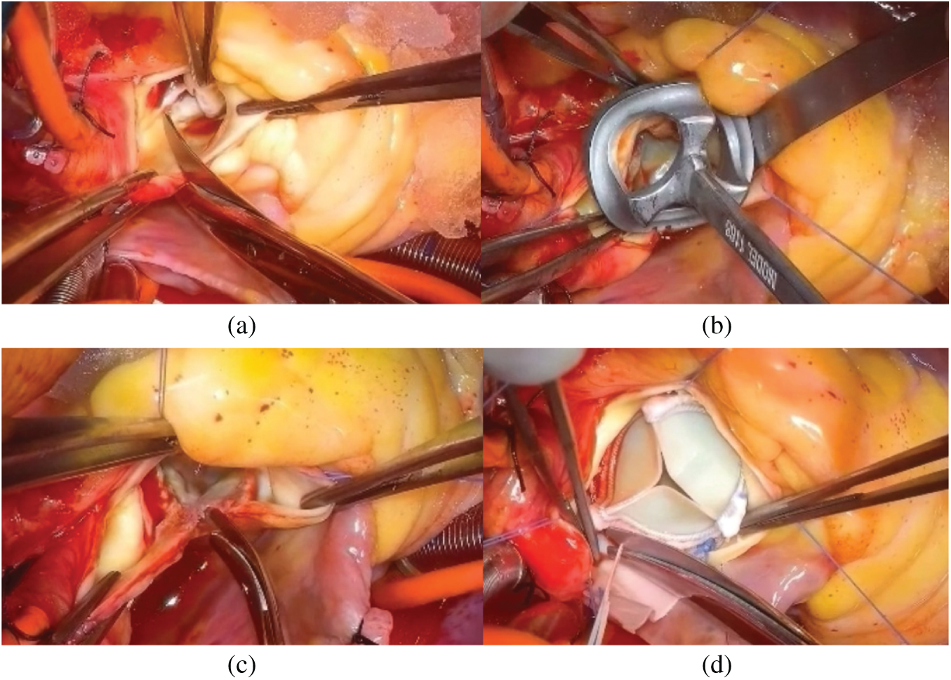
Figure 3: Main steps of aortic valve placement surgery with aortic root enlargement procedure. (a)Removing natural leaflets. (b) Sizing the aortic root. (c) Aortic root enlargement. (d) Placement of the prosthesis inside the aortic root

2.3 FSI Modeling and Boundary Conditions

2.3.1 The Structural Model and Aorta Root Material Properties

For aortic root structural model, we assumed that the aortic root material is hyperelastic, nearly-incompressible, homogeneous and anisotropic (valvular leaflets)/isotropic (aortic wall). The governing equations for aortic root models were as follows:

ρvi,tt=σij,j,i,j=1,2,3, (1)

εij=(vi,j+vj,i+vα,ivα,j)/2,i,j,α=1,2,3, (2)

where σ is the stress tensor, ρ is the material density, ε is the strain tensor, and ν is displacement. The normal stress was assumed to be zero on the outer (epicardial) aortic root surface and equal to the normal stress imposed by fluid forces on the inner (endocardial) aortic and leaflet innersurface.

The Mooney–Rivlin model was used to describe the nonlinear anisotropic (valvular leaflets) and isotropic (aortic wall) material properties. The strain energy function for the five-parameter Mooney–Rivlin model was given below [32]:

W=c1(I1-3)+c2(I2-3)+c3(I1-3)2+c4(I1-3)(I2-3)+c5(I2-3)2+1d1(I3-1)2(3)

where I1, and I2 are the first and second strain invariants,

I1=∑ Cii,I2=12(I12-CijCij),i,j=1,2,3,(4)

I3 = 1, C=[Cij]=FTF is the right Cauchy–Green deformation tensor. F=[Xij]=[∂xi/∂aj] where xi is the current location and aj is the original location. ci, i=1,…,5, and d1 are the material parameters, and aortic wall tissue Moony–Rivlin model parameter values were from Ranga et al. [32]. The strain energy function for the anisotropic modified Mooney–Rivlin model was given as [33–38]:

W=c1(I1-3)+c2(I2-3)+D1(eD2(I1-3)-1)+K1K2(eK2(I4-1)2-1)(5)

where I4=Cij(nf)i(nf)j, Cij is the Cauchy–Green deformation tensor, nf is the fiber direction, c1, c2, D1, D2, K1 and K2 are the material parameters, and the porcine pericardial tissues Moony–Rivlin constants c1, c2, D1, D2 K1 and K2 from Rassoli et al. [39] were used for leaflet tissues.

2.3.2 The Flow Model

Blood flow was assumed to be laminar, Newtonian, viscous and incompressible. The Navier–Stokes equations with ALE formulation were used as the governing equations. Our flow model is given below [35–38]:

ρ(∂u∂t+((u-ug)⋅∇)u)=-∇p+μ∇2u (6)

∇⋅u=0 (7)

uinlet=uinlet(t),p∣outlet=0 (8)

σij⋅nj∣out_wall=0 (9)

σijr⋅nj∣interface=σijs⋅nj∣interface (10)

σijr⋅nj∣interface=fluidstress,σijs⋅nj∣interface=structurestress. (11)

where u and p are fluid velocity and pressure, ug is mesh velocity. μ is the viscosity of blood, ρis blood density, Γ stands for aortic and leaflet inner wall, X is the structure displacement vector, σrand σs are fluid and structure stress tensors, and n is the surface outward normal direction. Inlet and outlet are subvalvular outflow tract (inlet) and ascending aorta (outlet). Blood density ρ and viscosity μ were set as ρ=1000 kg/m3 and μ=0.004 Pa⋅s, respectively.

2.3.3 Boundary Conditions

No-slip boundary conditions and natural force boundary conditions were specified at all interfaces to couple fluid and structure models together. Heart rate of the patient was 108 bpm. The systolic velocity waveform at the midpoint of the LVOT cross-section was measured by pulse Doppler (Fig. 2a). In our model, flow velocity at the inlet of root models was specified so that blood flow rate waveform matched measured patient data as shown in Fig. 2c. Blood pressure at the outlet was set as zero as currently done by some other researchers [40].

2.3.4 Mesh Generation and Solution Method

A geometry-fitting mesh generation technique was employed to generate meshes for aortic root with complex geometry [36]. In the boundary-fitting mesh construction process, the fluid and structure domains were divided into hundreds of small “volumes” so that boundary-fitting meshes could be generated. The FSI valve models used 4-node tetrahedral element type. The four structure models (from No. 19 to No. 25) had 16273, 14598, 16667, and 16822 elements, and the four fluid models had 82081, 105195, 119382 and 114309 elements, respectively. The common boundaries of the solid and fluid domains were defined as the interfaces of the FSI models in ADINA (ADINA R&D, Watertown, MA) to couple those domains. The Fully-coupled Two-Way FSI models were solved by ADINA using unstructured finite elements and the Newton-Raphson iteration method. We used direct computational two-way coupling method, which was reported to be better and more accurate for multi-physics problems [24]. Using the direct computational two-way coupling, also called the simultaneous solution method, the equations of fluid flow and displacement of the solid are solved simultaneously by a single solver [24,41,42]. No-slip boundary conditions was specified at all interfaces to couple fluid and structure models together [41,42]. During FSI simulation, the tolerances for stress and displacement convergences were set as 0.01. Three cardiac cycles were simulated since the second and third cycles were almost identical. The third cycle was used for analysis. The simulations were performed on a workstation with Intel(R) Core(TM) i9-9900K 3.60 GHz processors.

2.4 Surgical Benchmark for Valve Size Optimization

Hemodynamics plays an important role in valve cardiac functions [2,16]. Surgeons often use mean systolic transvalvular pressure difference, peak systolic transvalvular pressure difference and geometric orifice area to assess and optimize AVR procedures, including selection of valve sizes. It is commonly agreed that lower systolic transvalvular pressure gradient, greater geometric orifice area, and lower shear stress after AVR would lead to better hemodynamic performance, extended valve durability, and improved long-term function of the valve. Those parameters were obtained using our FSI models to compare the functions of valves with different sizes.

2.5 Research Design

FSI models with 4 different valve sizes were used in this study to quantify transvalvular pressure gradient, flow shear stress and geometric orifice area from those models with the goal to optimize valve size selections in AVR. Blood flow velocity and aorta root dimension were obtained from one patient for modeling use. FSI aortic root models with 4 different bioprosthetic valve sizes (19, 21, 23 and 25 mm) were constructed to evaluate the impact of prosthetic valve size on AVR outcome. The systolic transvalvular pressure gradient and geometric orifice area were calculated to seek the optimal surgical design for potential AVR outcome improvements. The flow shear stress conditions on the leaflets were calculated which could provide important information for AVR design and improve the durability of bioprosthetic valve.

3  Results

Blood pressure, velocity, systolic valve orifice pressure gradient, systolic cross-valve pressure difference, geometric orifice area and flow shear stress of 4 valves models with different sizes were compared. Details are given below.

3.1 The Pressure and Velocity

Fig. 4 showed pressure and flow velocity plots at the peak systole of a cardiac cycle from the 4 valve models with different sizes. A longitudinal cross-section of the valve was selected to present the pressure and velocity contour plots showing their distribution patterns. While both pressure and velocity distributions from the 4 valve models showed similar patterns, maximum pressure and velocity from Valve No. 19 were 93.8% and 80.5% higher than those from Valve No.25, respectively (87.8 mmHg vs. 45.3 mmHg and 318.8 cm/s vs. 176.6 cm/s).

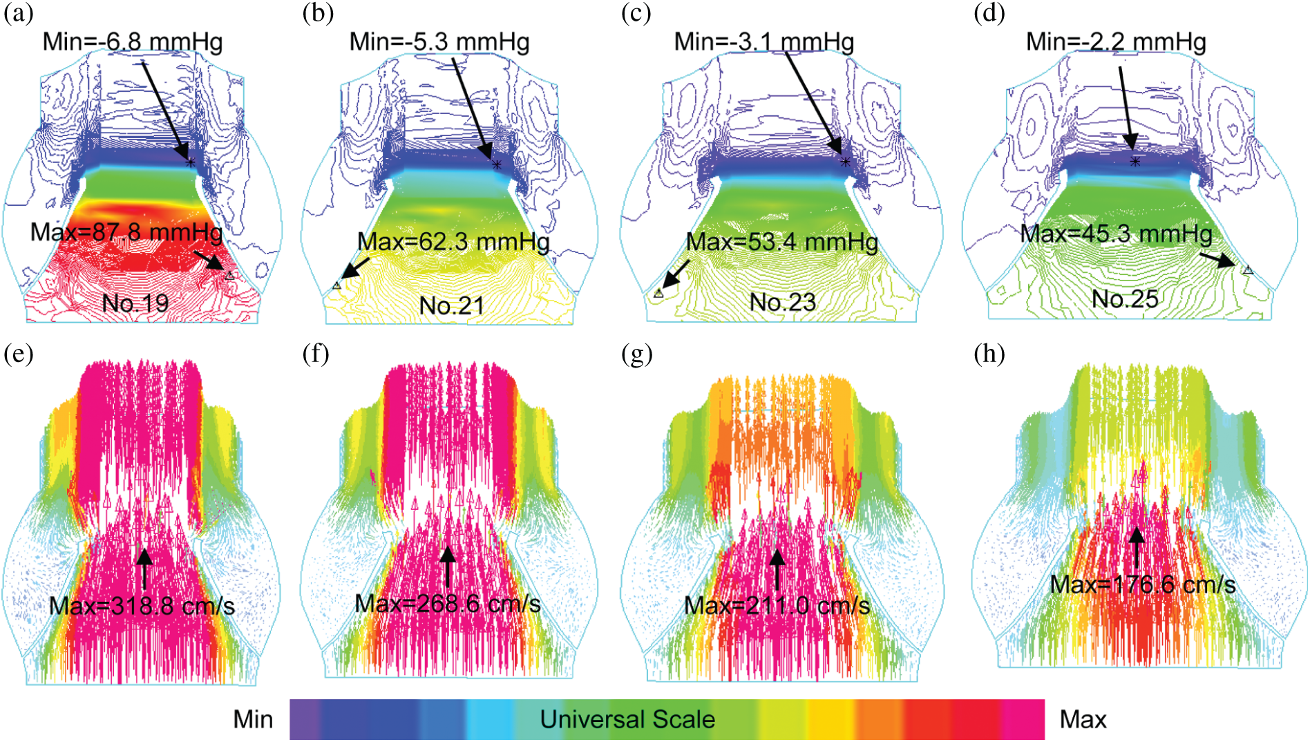
Figure 4: Blood pressure contour and velocity vector plots from the 4 valve models with valves fully open. (a–d): Pressure contour plots; (e–h): Velocity vector plots

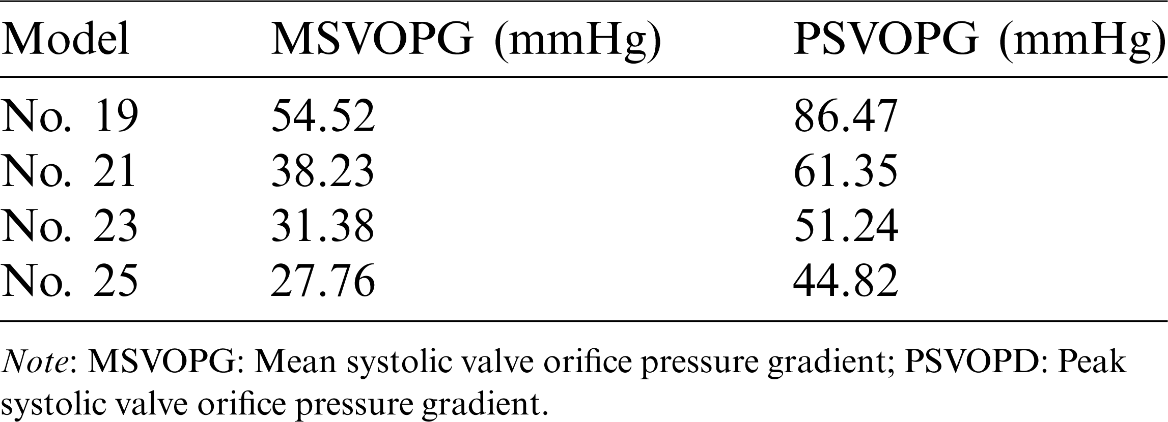
3.2 The Systolic Valve Orifice Pressure Gradient

Computational blood pressure values at an annulus cross-section and a sinotubular junction cross-section of valves were recorded and averaged over those cross-sections for analysis (Fig. 5a). Systolic valve orifice pressure gradient (SVOPG) was defined as the difference of the pressure values from the two cross-sections. Fig. 5 provided SVOPG waveforms obtained from the 4 valve models showing valves with smaller sizes had greater orifice pressure gradient. The time-averaged mean pressure gradient and the peak pressure gradient values are shown in Tab. 2. It is clear from Fig. 5d that SVOPG from Valve No. 25 was the lowest among the 4, only 51.83% of that from Valve No. 19 (maximum 44.82 mmHg vs. maximum 86.47 mmHg). While the locations of the selected cross-sections in the calculation will affect the pressure value, results for the relative differences of those valves should remain valid.

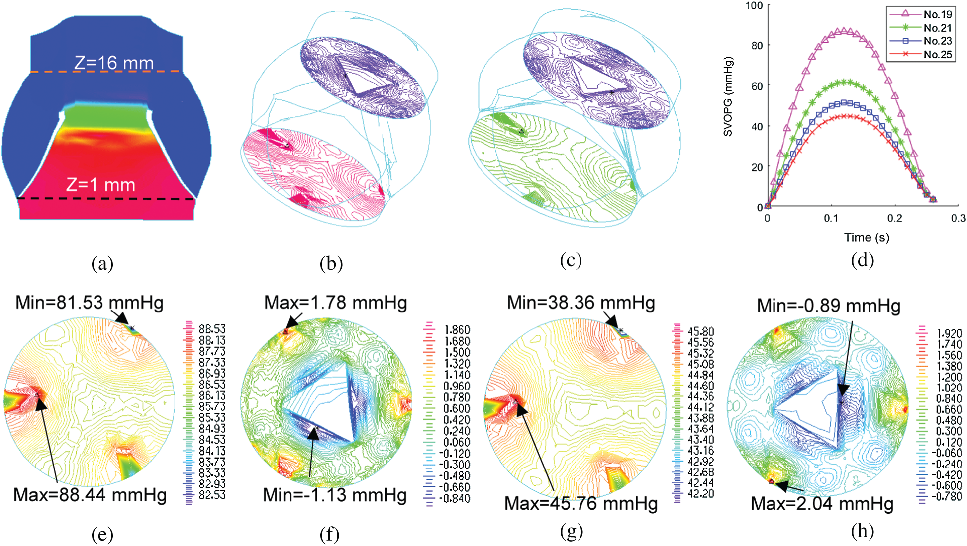
Figure 5: Systolic valve orifice pressure gradient (SVOPG) obtained from FSI simulations. (a)Location of two cross-sections selected for SVOPG calculation. (b and c) are 3D views of the aorta root when the valve was fully open with two cross-section pressure contour plots included. (b)is Valve No. 19. (c) is Valve No. 25. (d) The SVOPG profiles from the 4 FSI models during systole. (e and f) are pressure contour plots of No. 19 at Z = 1 mm (e) and Z = 16 mm (f), respectively. (g and h) are pressure contour plots of No. 25 at Z = 1 mm (g) and Z = 16 mm (h), respectively. Different color scale was used for each plot for (e–h) to show pressure field details since pressure variations on each cross-section were small

Table 2: The systolic valve orifice pressure gradient calculated from the results of FSI simulations

3.3 The Systolic Cross-Valve Pressure Difference

The true forces that the valve leaflets are subjected to are determined by the flow pressures on the two sides of the leaflets: The side facing LV (inlet) and the side facing aorta (outlet). Flow pressure data on the two sides from the FSI models (they are actually the FSI interfaces between the flow model and the structure model) were recorded and averaged (over the leaflets) for comparison analysis. The systolic cross-valve pressure difference (SCVPD) was the pressure difference from the two sides of the leaflets. Fig. 6 compared the mean (over time) SCVPD and peak SCVPD for the four valves during the systolic phases. As the valve size increased, both peak SCVPD and mean SCVPD decreased. Peak SCVPD of Valve No. 25 was 36.3 mmHg, 48.1% lower than that from Valve No. 19 (70.0 mmHg). Similarly, mean SCVPD from Valve No. 25 was 22.5 mmHg, 49.3% lower than that from Valve No. 19 (44.4 mmHg).

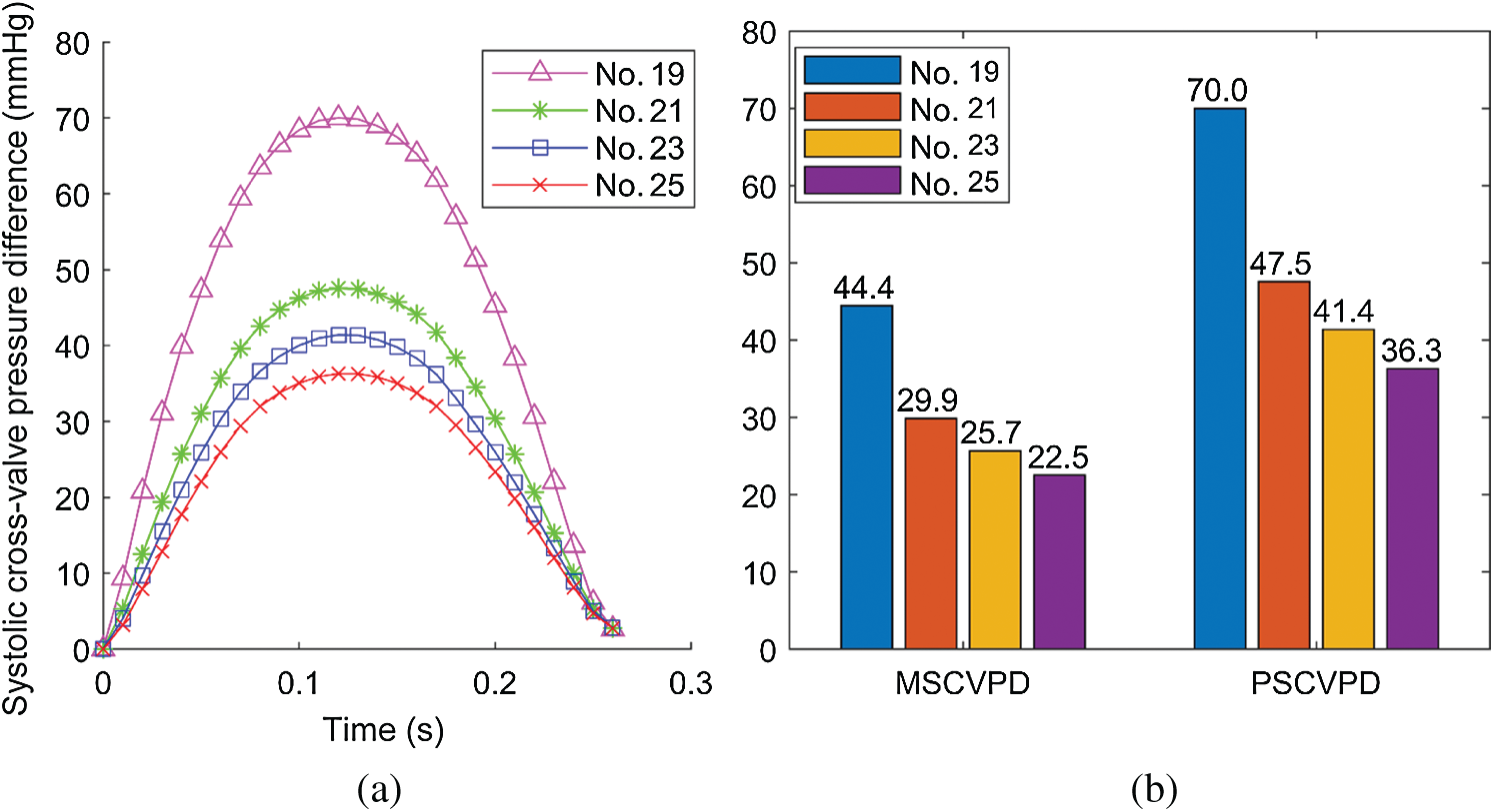
Figure 6: Systolic cross-valve pressure difference calculated from the results of FSI simulations. (a) The systolic cross-valve pressure difference waveforms of different valve sizes. (b) Comparison of mean systolic cross-valve pressure difference (MSCVPD) and peak systolic cross-valve pressure difference (PSCVPD) among the four models. Unit: mmHg

3.4 The Geometric Orifice Area

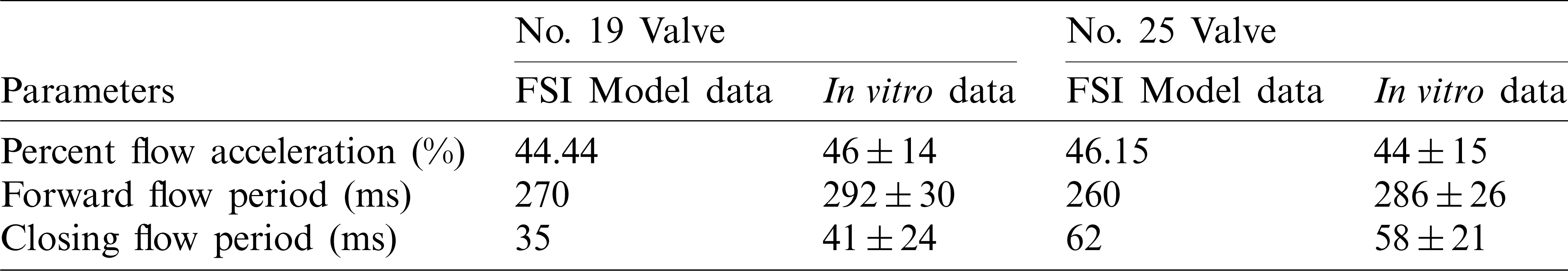
Geometric orifice area (GOA) was used as the main parameter to assess valve kinematics. It was calculated directly from the deformed valve geometry [16]. The GOA of valves from the 4 models were shown in Fig. 7. Valves with larger sizes had larger geometric orifice areas, with Valve No. 25 giving the maximum value 1.87 cm2, 52.03% higher than that of Valve No. 19 (1.23 cm2). Additionally, we estimated forward acceleration period and forward flow period to analyze the valve motion pattern. Forward acceleration period, forward flow period and closing flow period are defined as time durations from start forward flow to peak forward flow, from start forward flow to end forward flow and end forward flow to end closing flow, respectively [43]. The percent flow acceleration is flow acceleration period divided by forward flow period. FSI model results and in vitro measurements for valve size No. 19 (minimum size) and No. 25 (maximum size) were listed in Tab. 3. Tab. 3 confirmed the consistency of FSI model results with in vitro measurements.

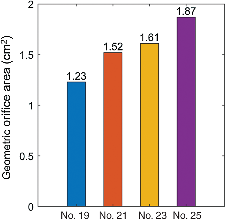
Figure 7: The geometric orifice area plots from the 4 valve models with valves fully open

Table 3: Comparison of percent forward acceleration, forward flow period and closing flow period between our FSI models and measured in vitro [43]

3.5 The Flow Shear Stress

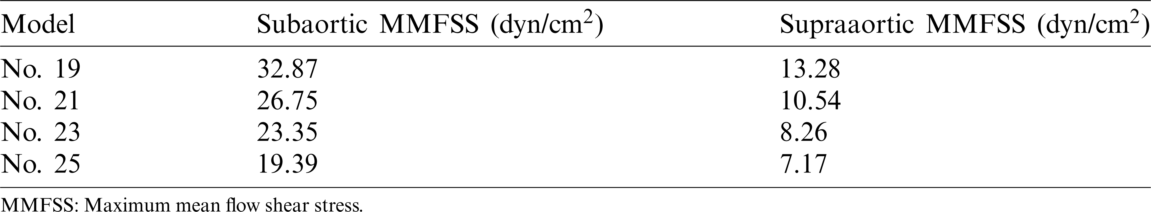
Flow shear stress (FSS) on valve leaflet surface plays an important role in valve functions, disease initiation, development and healing. FSS on all nodes on the supraaortic surface (the side of the leaflets facing aorta) and the subaortic surface (the side of the leaflets facing LV) were recorded, and mean FSS (averaged on the two leaflet surfaces, respectively) were obtained foranalysis. Time-varying mean FSS values in systolic phase are plotted in Fig. 8. The maximum values of those curves are given in Tab. 4. Tab. 4 shows that the subaortic maximum mean flow shear stress (MMFSS) was significantly higher than the supraaortic MMFSS for all 4 valve models (147.5%, 153.8%, 182.7%, and 170.4% for No. 19, No. 21, No. 23, and No. 25, respectively). Valves with larger sizes had lower MMFSS. Supraaortic MMFSS and subaortic MMFSS for Valve No. 25 were 46.00% and 41.01% lower than that from Valve No. 19, respectively. Our results indicated that implantation of larger valves could significantly reduce mean flow shear stress.

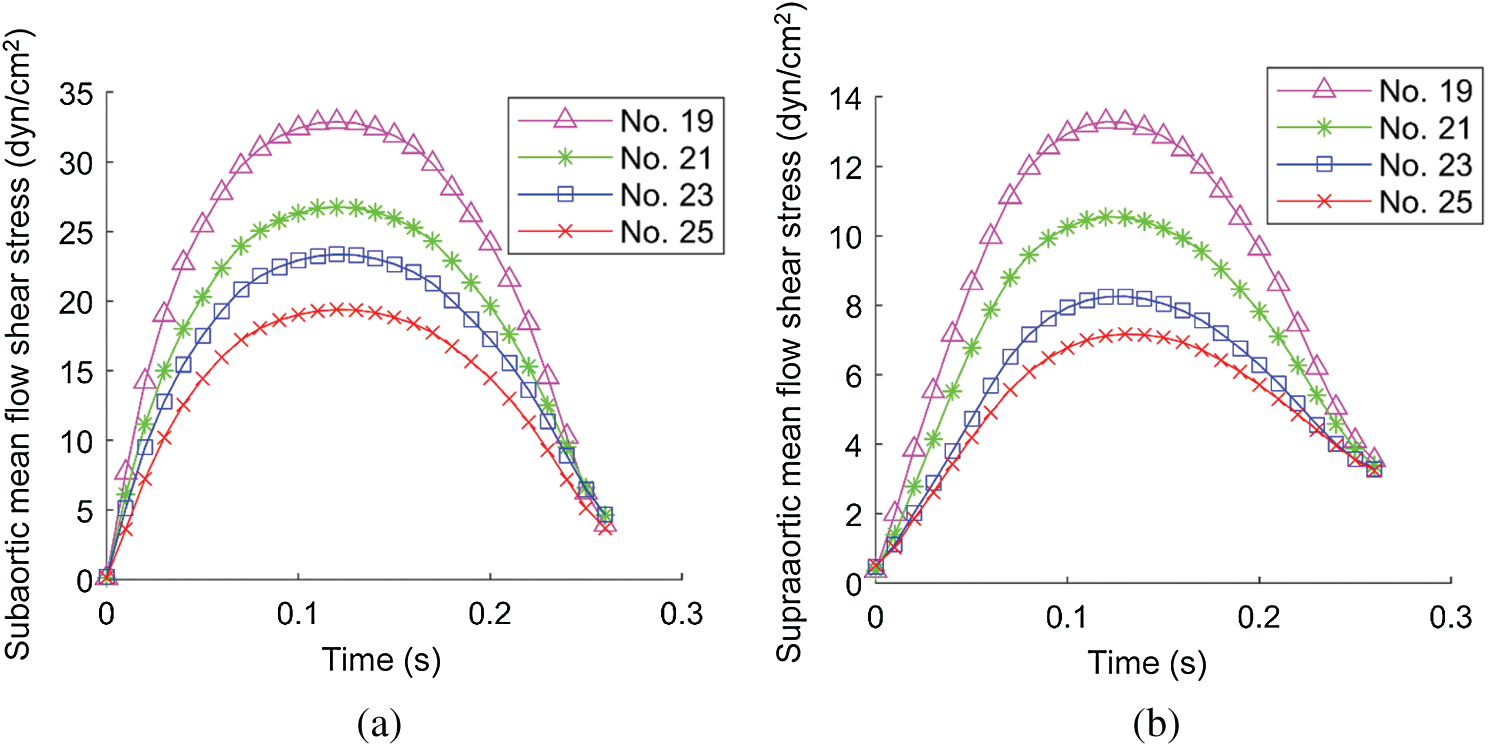
Figure 8: Systolic mean flow shear stress (MFSS) on the leaflet surface. (a) The systolic MFSS on the subaortic surface. (b) The systolic MFSS on the supraaortic surface

Table 4: The maximum mean flow shear stress of different valve sizes on the valve

4  Discussion

4.1 Computational Valve Model as a Tool for Potential Use in Optimizing AVR Outcome

This study applied a FSI modeling approach to patients undergoing AVR to investigate the effect of valve size on the outcome of AVR surgery. The computational modeling approach could be using to test the feasibility of novel high-risk surgical procedures to avoid performing those surgical procedures on humans. Aortic root valve FSI models were built sharing the same material properties of aortic root and inlet flow rate to simulate the AVR with different valve sizes for the same patient. Non-linear anisotropic material model was used to characterize the mechanical properties of aortic valve leaflets, which is consistent with the anisotropic properties of aortic valve leaflets reported in literature [10,39,44]. Our results indicated that implanted larger valves led to lower hemodynamic transvalvular pressure gradient, lower flow shear stress and larger geometric orifice area. The FSI models could be used as tools to analyze clinically relevant problems, optimize surgical procedures, and improve AVR outcome.

4.2 Morphological and Hemodynamic Factors in Optimizing Aortic Valve Replacement Surgical Outcome

In both routine clinical and research applications, evaluations of the hemodynamic performance of bioprosthetic valves are mainly focused on transprosthetic pressure gradient and orifice area which directly affect ventricle cardiac function [45]. Therefore, flow pressure, velocity, SVOPG, SCVPD, FSS and GOA were obtained using our FSI models and used for our valve comparisons. Our results demonstrated that larger valves led to lower maximum velocity, pressure, SVOPG and SCVPD (Figs. 4–6). Valve No. 25 had 44.60% lower maximum velocity, 48.41% lower maximum pressure, 48.17% lower peak SVOPG, and 49.32% lower mean SCVPD versus the No. 19 valve. Distribution patterns of pressure and velocity from the 4 valve models on the longitudinal cross-section were similar. These pressure and velocity distribution patterns were consistent with the literature [27,46].

Kinematics of the valves with different sizes were compared by GOA (Fig. 7). During systole, the valve commissures were pushed outward by strong unidirectional flow jet, therefore stretching the leaflets and forming a triangular opening. Our results showed that the larger size of valve allows for larger GOA, with Valve No. 25 (1.87 cm2) being the largest, 52.03% larger than Valve No. 19 (1.23 cm2).

FSS is closely related to ventricle remodeling and valve disease initiation and development such as inflammation and calcification. Fig. 8 showed that during systole subaortic surface (ventricular side) was exposed to higher FSS levels than supraaortic surface (aortic side) for all 4 valve models, which was consistent with literature [16]. FSS values were low during early systole and late-systole, and reached the maximum during mid-systole. We also observed that implantation of larger valves can significantly reduce mean flow shear stress during systole.

4.3 Model Limitations and Future Directions

Our first major limitation is that image-based patient-specific 3D valve geometry reconstruction was not included and data from root bioprosthesis and previous work were used [31]. Imaging valve leaflet geometry under in vivo conditions is challenging with current technology. Reconstructing the 3D geometry of the aortic root based on patient-specific data will be our next step in our research. The second limitation is that zero pressure outlet condition was used which should be replaced by actual time-dependent aortic pressure conditions. While this had only minor effect on transvalvular pressure gradients, actual pressure conditions should still be used to obtain correct aortic root structure stress/strain conditions. The third limitation is that our current aortic root model should be fully coupled with ventricle model to include ventricle and valve interactions so that the model would be more realistic.

Funding Statement: The research was supported in part by National Sciences Foundation of China Grants 11672001, 81571691 and 81771844.

Conflicts of Interest: The authors declare that they have no conflicts of interest to report regarding the present study.

This work is licensed under a Creative Commons Attribution 4.0 International License, which permits unrestricted use, distribution, and reproduction in any medium, provided the original work is properly cited.