| Computer Modeling in Engineering & Sciences |
DOI: 10.32604/cmes.2021.012720
ARTICLE
Redefined Extended Cubic B-Spline Functions for Numerical Solution of Time-Fractional Telegraph Equation
1Department of Mathematics, National College of Business Administration & Economics, Lahore, 54660, Pakistan
2Department of Mathematics, University of Sargodha, Sargodha, 40100, Pakistan
3Department of Mathematics, Faculty of Arts and Sciences, Cankaya University, Ankara, 06530, Turkey
4Department of Medical Research, China Medical University Hospital, China Medical University, Taichung, 40402, Taiwan
5Institute of Space-Sciences, Bucharest, 077125, Romania
6Department of Mathematics, Government College University, Faisalabad, 38000, Pakistan
7Department of Mathematics, University of Management and Technology, Lahore, 54700, Pakistan
*Corresponding Author: Muhammad Abbas. Email: muhammad.abbas@uos.edu.pk
Received: 10 July 2020; Accepted: 21 December 2020
Abstract: This work is concerned with the application of a redefined set of extended uniform cubic B-spline (RECBS) functions for the numerical treatment of time-fractional Telegraph equation. The presented technique engages finite difference formulation for discretizing the Caputo time-fractional derivatives and RECBS functions to interpolate the solution curve along the spatial grid. Stability analysis of the scheme is provided to ensure that the errors do not amplify during the execution of the numerical procedure. The derivation of uniform convergence has also been presented. Some computational experiments are executed to verify the theoretical considerations. Numerical results are compared with the existing schemes and it is concluded that the present scheme returns superior outcomes on the topic.
Keywords: Extended cubic B-spline; redefined extended cubic B-spline; time fractional telegraph equation; caputo fractional derivative; finite difference method; convergence
In recent years, fractional calculus has gained a remarkable importance. Fractional derivatives and integrals have manifold applications in science and engineering such as fluid mechanics, chemical physics, electricity, control theory, biomedical, epidemic diseases, hydrology, electro-chemistry, probability theory, signal processing, heat conduction and diffusion problems [1–7]. Many researchers developed fractional-order models to describe real-world problems and studied their analytical and numerical solutions [8–11]. These models involve different types of fractional derivative operators [12–15]. The fractional telegraph equation is one of the fundamental mathematical models arising in the study of electrical signals in transmission line and wave phenomena [16–18]. Basically, it belongs to the family of hyperbolic partial differential equations. Several numerical and analytical techniques have been proposed for solving these type of equations. In [19], the authors employed Adomian decomposition method for solving time and space fractional telegraph equations. Dehghan et al. [20] proposed variational method to explore the series solution to multi space telegraph equation. The authors in [21], employed Homotopy analysis method to explore the analytical solution of telegraph equation involving fractional time derivative. Later on, Hayat et al. [22] used Homotopy perturbation technique to study time fractional telegraph equation. They handled TFTE for both brownian and standard motion. In [23], Wei et al. applied fully discrete local discontinuous Galerkin finite element method to solve fractional telegraph equation. Hosseini et al. [24] studied the numerical solution of fractional telegraph equation by means of radial basis functions. Srivastava et al. [25] employed reduced differential transformation method for second order hyperbolic time fractional telegraph equation in one dimensional space. Wang et al. [26] analyzed an H1-Galerkin mixed finite element method for the numerical solution of time fractional telegraph equation. Modanli et al. [27] solved fractional order telegraph equation by means of Theta method. Xu et al. [28] applied Legendre wavelets direct method for solving fractional order telegraph equation. In [29], Wang et al. utilized spectral Galerkin approximation to study the approximate solution of TFTE. Kamran et al. [30] studied the numerical solution of TFTE by means of a Localized kernal-based approach. Here, in this work, we consider the following fractional order telegraph equation.
where
In this paper, we have studied the application of a redefined form of extended cubic B-spline (ECBS) functions for the numerical treatment of time-fractional Telegraph equation (TFTE). These functions are generalized forms of cubic B-spline functions involving one free shape parameter which provides the flexibility to modify the shape of the solution curve [31]. Although, the degree of the piecewise polynomials is enhanced by one and the continuity of RECBS remains of order three. A finite-difference formula is used for the discretization of the Caputo time-fractional derivative. Usually, in collocation techniques, the Dirichlet’s type end conditions are imposed where the basis of spline functions vanish, but the typical ECBS functions do not vanish at boundaries. We have employed RECBS functions for spatial discretization, as these basis functions die out on the boundaries where the Dirichlet’s types of conditions are specified. The present approach is novel for the approximate solution of fractional PDEs and as far as we are aware, it has never been employed for this purpose before.
The manuscript is composed as: Section 2 describes the redefined extended cubic B-spline functions. In Section 3, the numerical method has been explained. In Section 4, the stability analysis of proposed method is presented. In Section 5, we have derived the results for theoretical convergence. The approximate results and discussion are reported in Section 6. Finally, the concluding remarks have been given in Section 7.
2 Redefined Extended Cubic B-Spline Functions
Suppose the spatial domain
where
where
where
where the weight function
We divide the time domain
where
Also
where
•
•
•
Similarly,
where
Also
where
•
•
•
Substituting (10) and (12) in (1) at t = tr+1, we get
Using theta-weighted scheme for
where
For r = 0, v−1 appears in Eq. (15). We use the initial conditions and substitute
For
Now, we discretize the spatial domain [a, b] by M + 1 equally spaced knots
where
Solution at t = t1
The initial solution is given in (2). However, the control points
Solving (19), we get
Solution at
Using (18) in Eq. (17), we obtain
Eq. (20) represents a set of (M + 1) equations involving (M + 1) unknowns. This system of equations is solved to for
We apply Fourier method to study the stability of our numerical method. Let
where
If
After simplifying (23), we get the following result
where
For r = 0, the expression (23) takes the following form
Now, assuming
Consequently, following [34], we have
Hence, the scheme stable.
Let
where
The boundary conditions can be rewritten as
Moreover, following [34], we have
Therefore,
Now, we introduce
Involving the absolute values of
Hence, employing the end constraints, we get
Now, assuming that
Utilizing the boundary conditions, we obtain
Hence, the last result is true for all r. Using the result
Consequently, using (26) and (27), we get
Hence, in the light of above discussion together with (11) and (13), we conclude that the scheme is O(h2) accurate in spatial direction. However, (11) and (12) imply that the truncation error in temporal direction is
To investigate the accuracy of presented technique, some numerical experiments are presented. For this purpose, following error norms have been used
Also, the experimental order of convergence (EOC) is computed by following important formula [35]:
Example 6.1. As the first experiment, we take the following multi term TFTE [29]
The exact solution of the problem is
The absolute error and temporal order of convergence for Example 6.1 along temporal direction using M = 24 and different values of
Table 1: Experimental order of convergence (EOC) for Example 6.1 when M = 24 using different values of
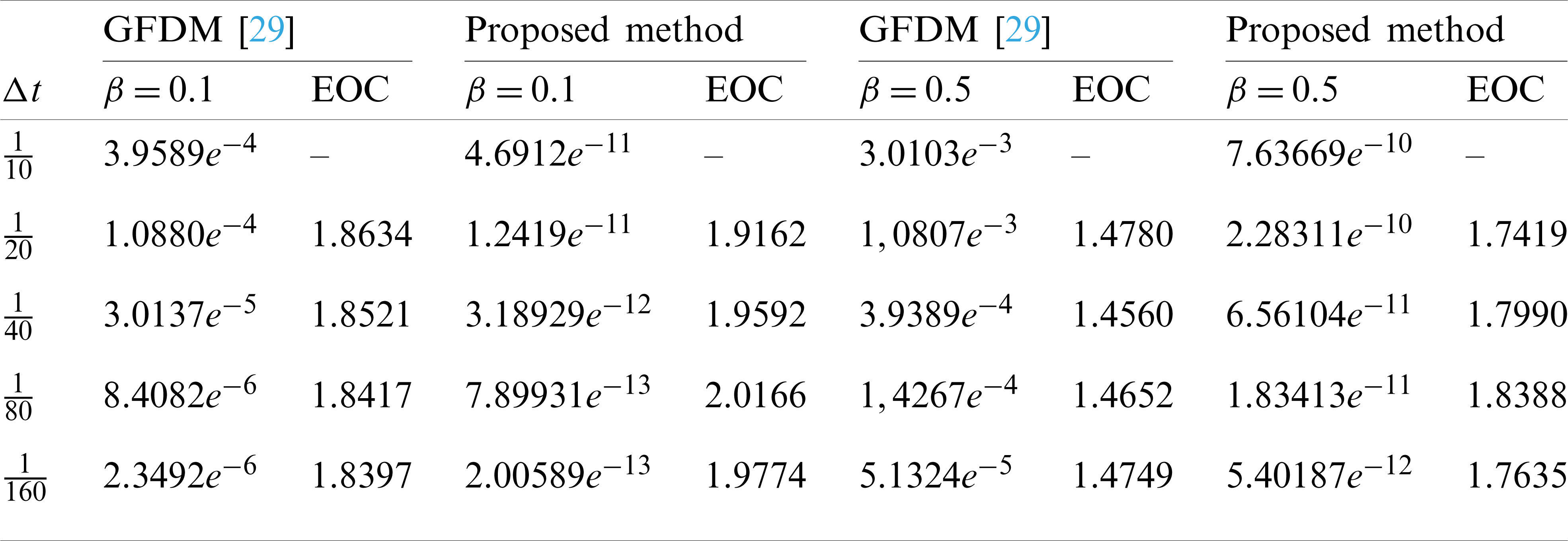
Table 2: Absolute errors for Example 6.1 when
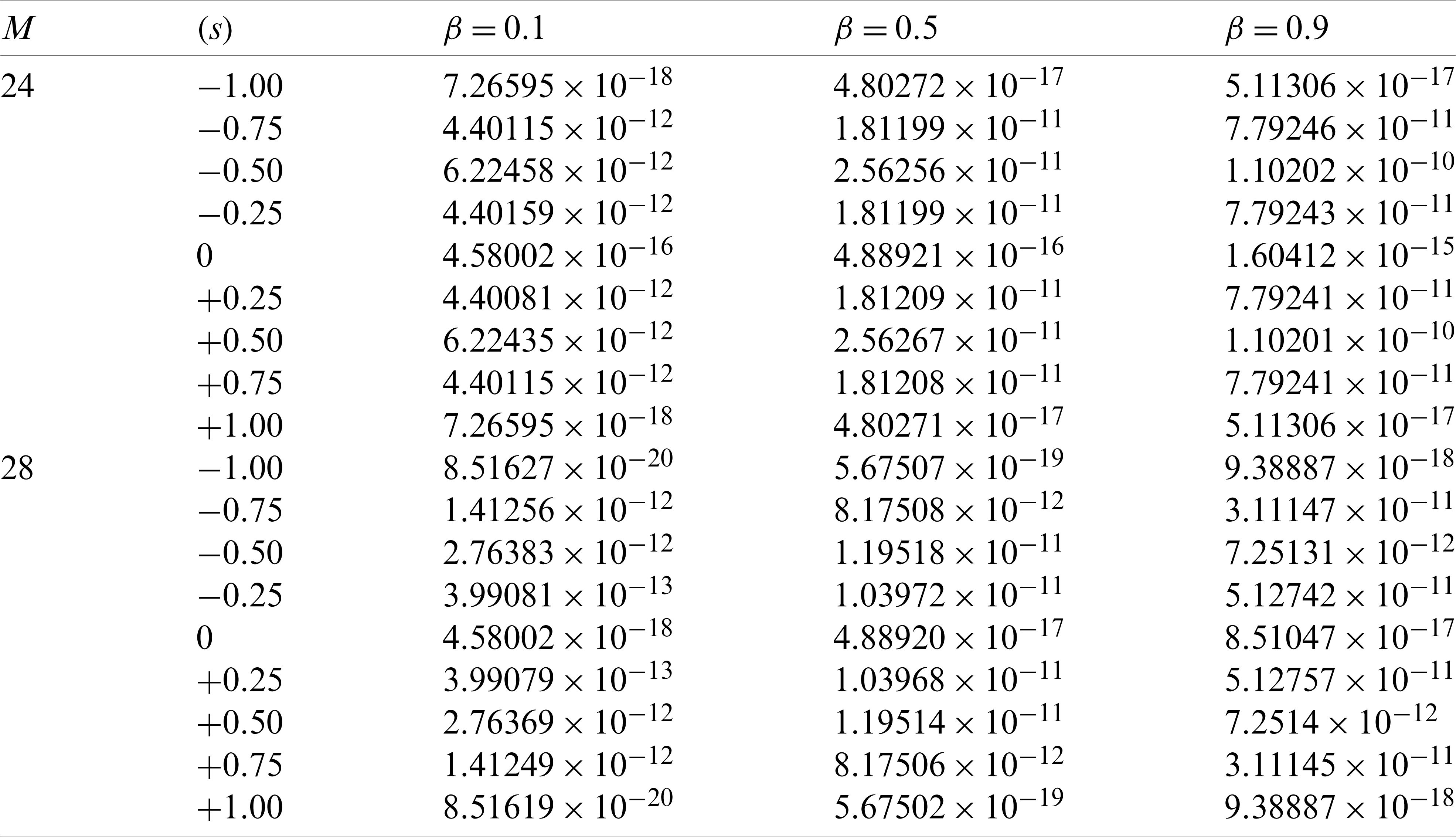
Table 3: Experimental order of convergence (EOC) for Example 6.1, when
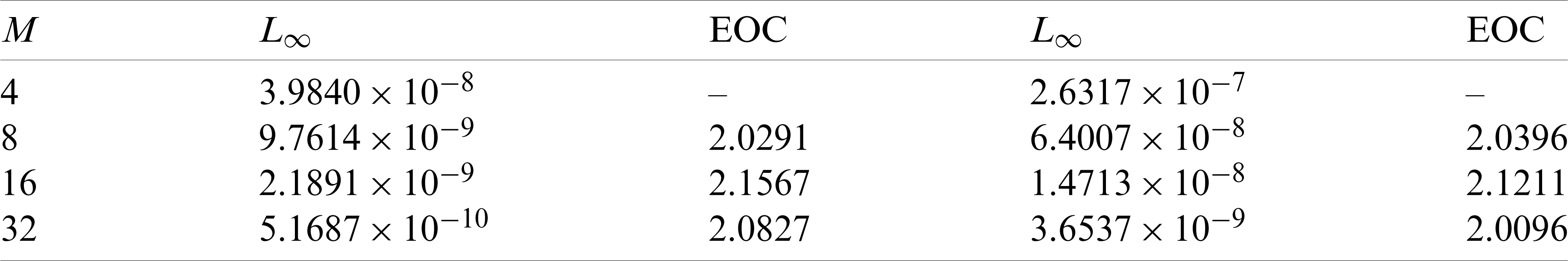
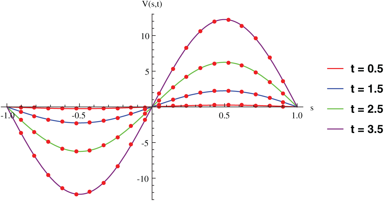
Figure 1: Exact and numerical solution for Example 6.1 at different time levels when
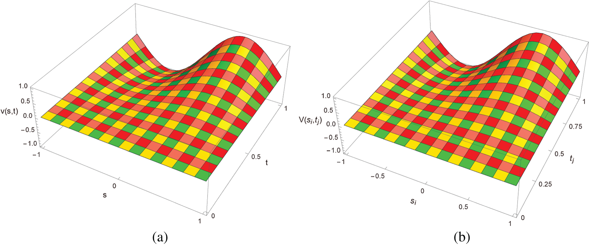
Figure 2: Exact and approximate solution for Example 6.1 with M = 24,
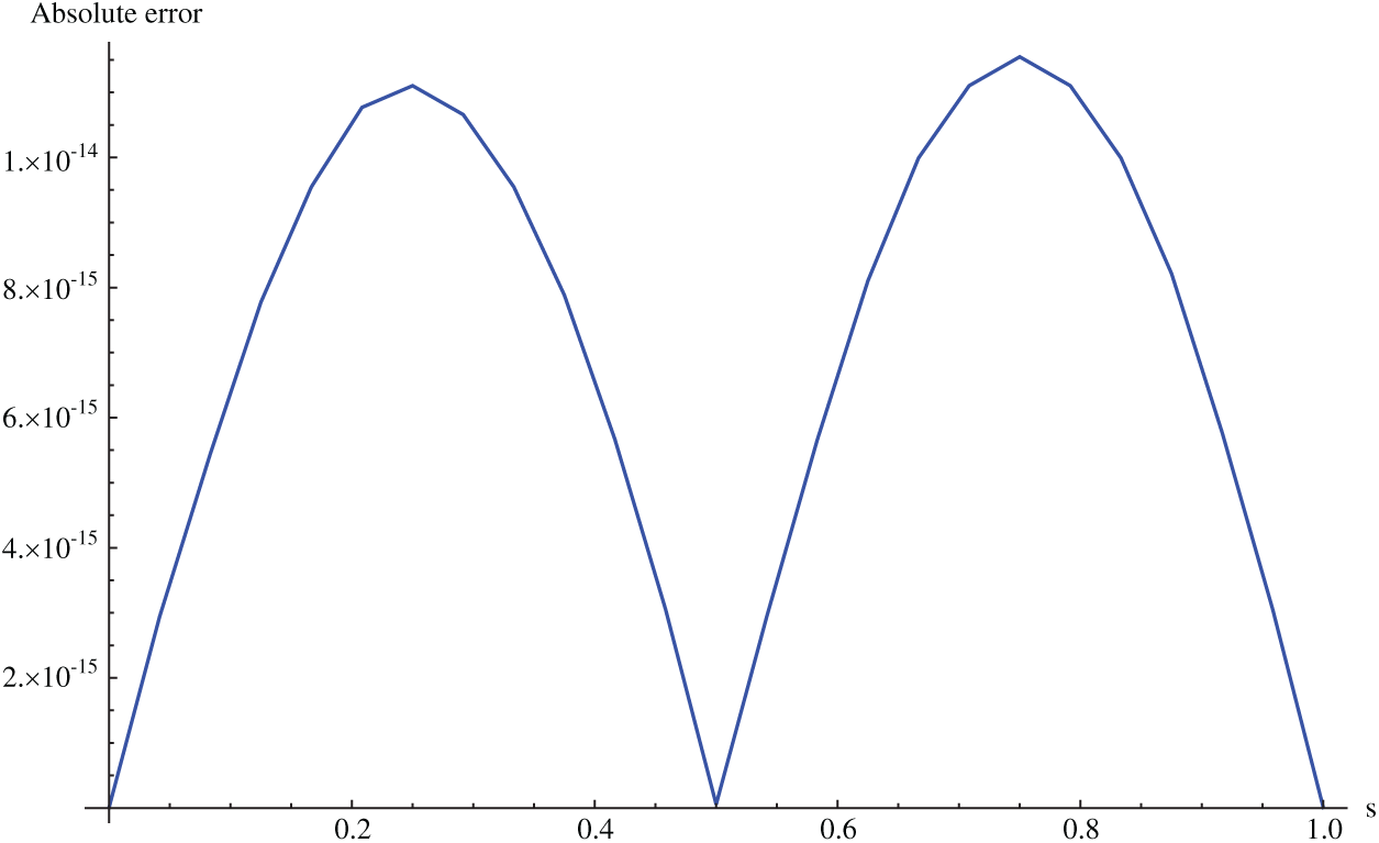
Figure 3: Absolute error for Example 6.1 when M = 36,
The piecewise defined approximate solution for Example 6.1 using proposed algorithm, when
Example 6.2. Consider the TFTE [27]
The analytical solution to this problem is
The approximate analytical solution for Example 6.2 using proposed method, when
The absolute numerical errors in RECBS solution for Example 6.2 setting
Table 4: Absolute error norms for Example 6.2 using different values of M and
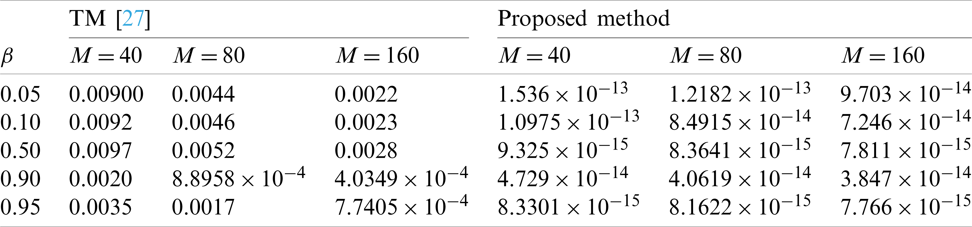
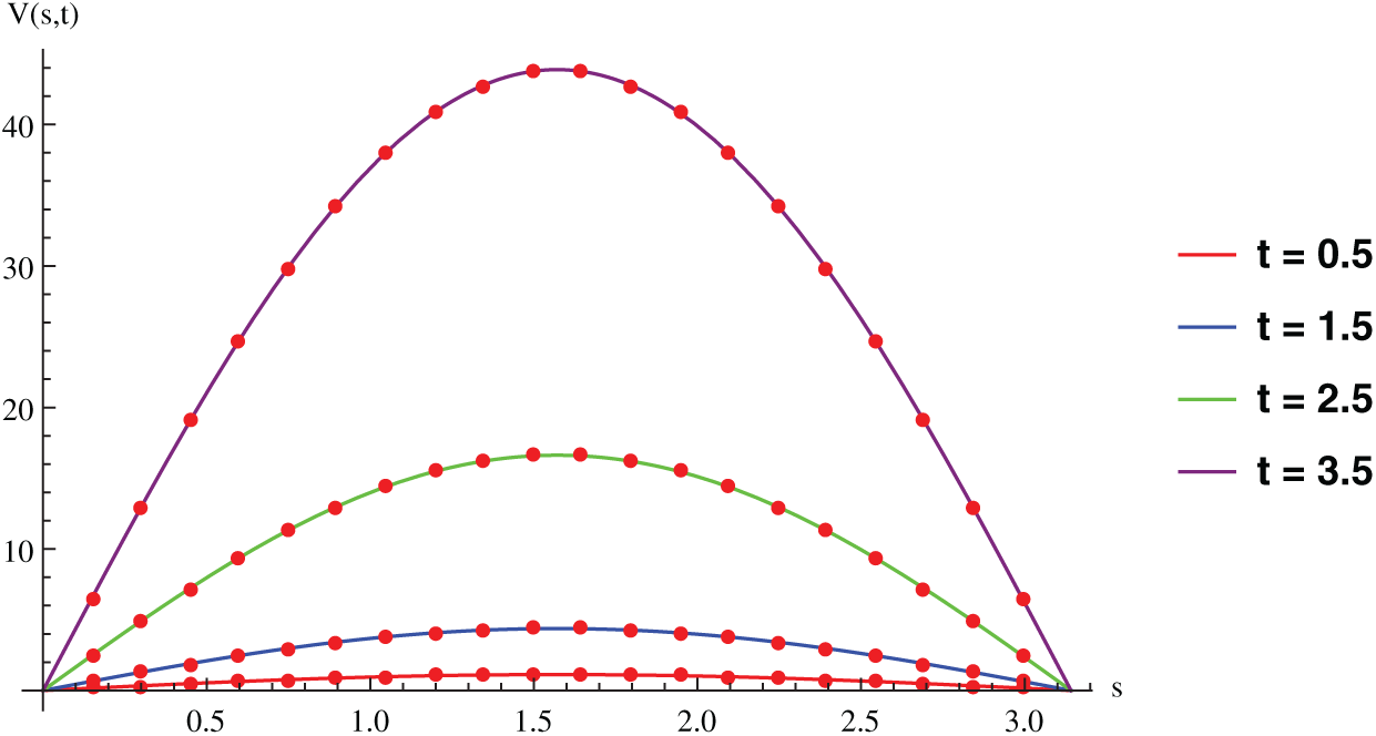
Figure 4: Exact and numerical solution for Example 6.2 at different time levels when
Example 6.3 Consider the multi term TFTE [30]
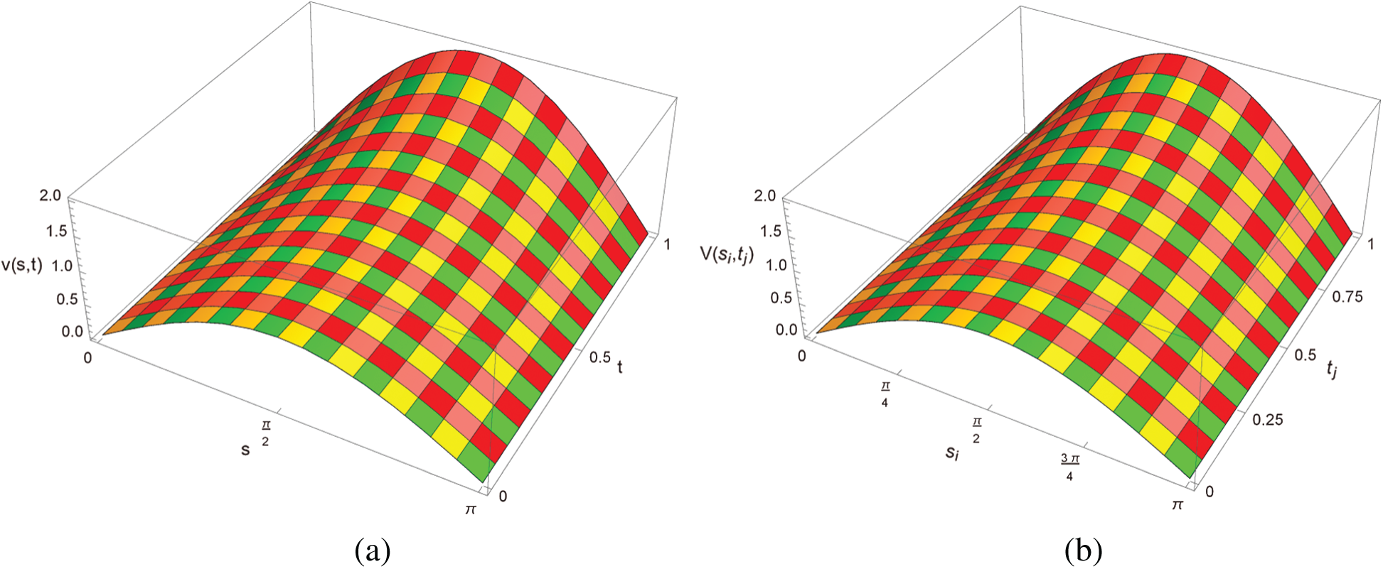
Figure 5: Exact and approximate solution for Example 6.2 with
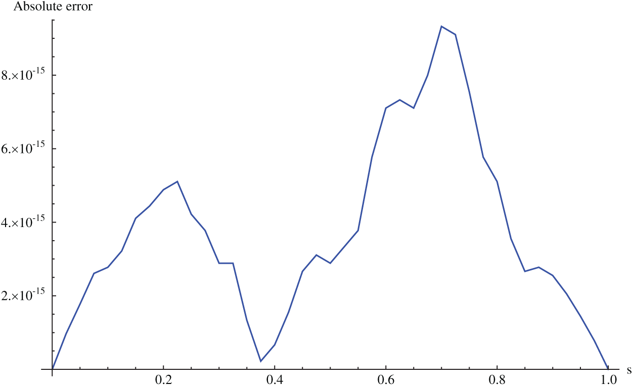
Figure 6: Absolute error for Example 6.2 when M = 40,
The exact solution is (s2 − s)t.
The numerical solution for Example 6.3, when
The absolute numerical errors in RECBS solution to Example 6.3 using
Table 5: Absolute error for Example 6.3 when
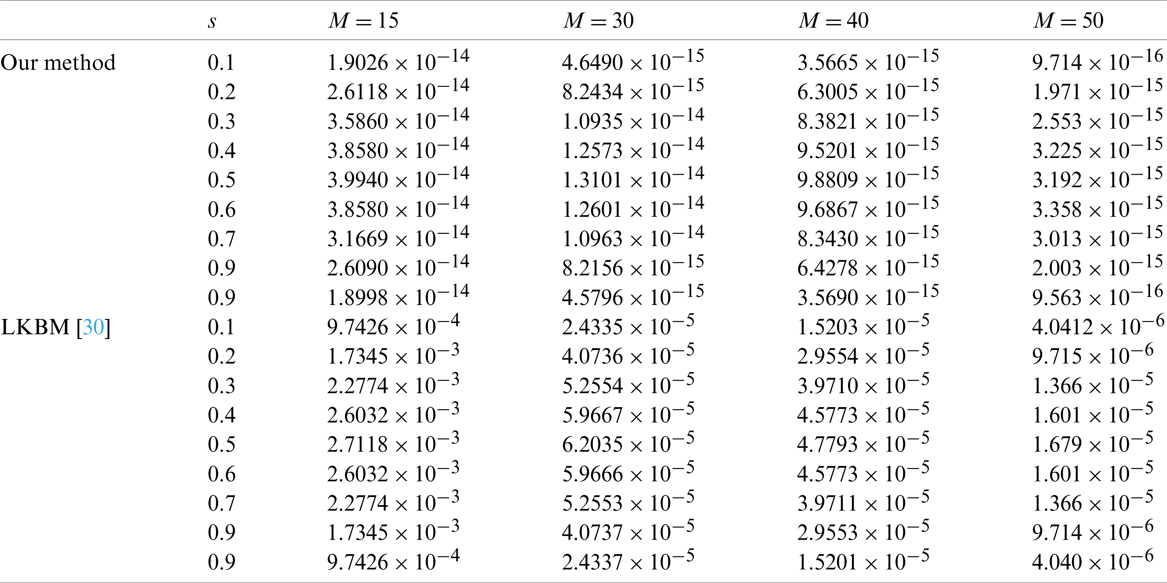
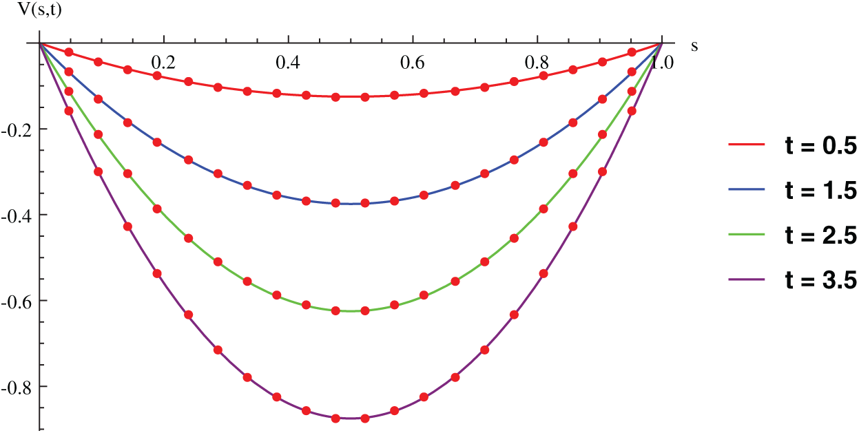
Figure 7: Exact and numerical solution for Example 6.3 at different time levels when
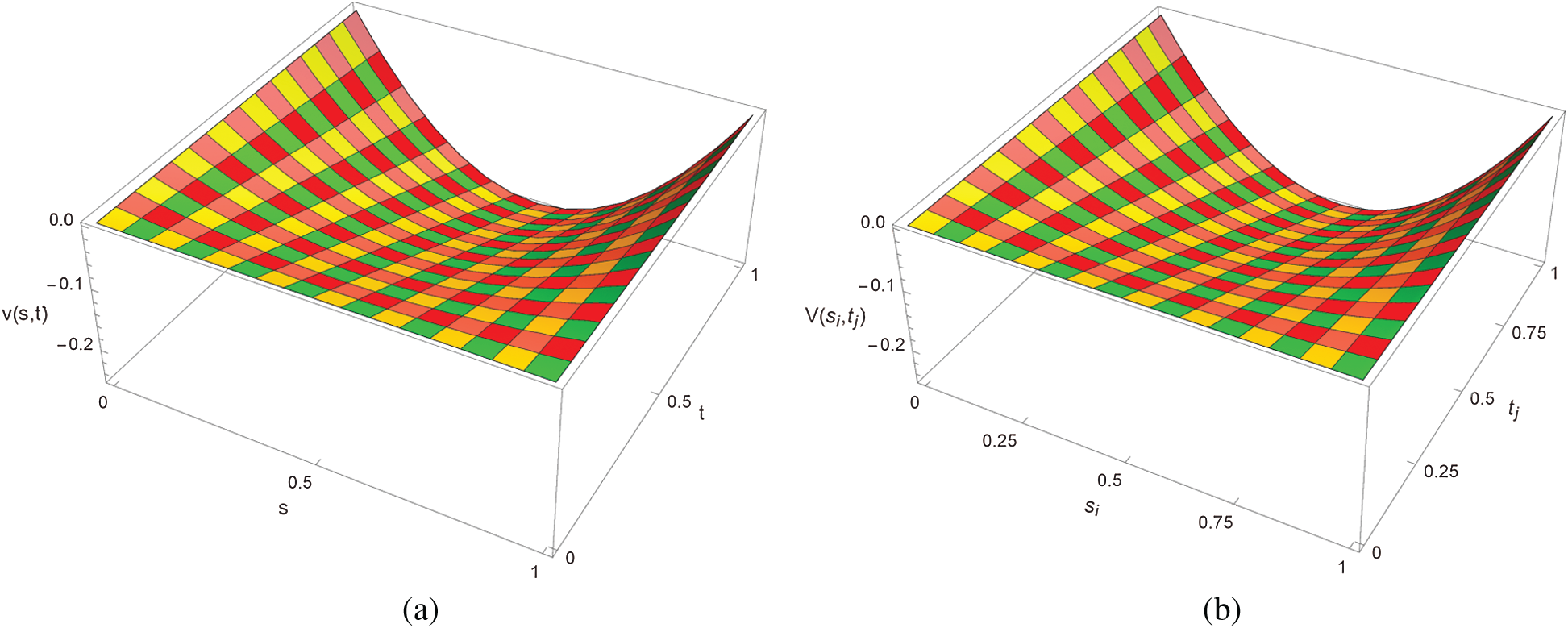
Figure 8: Exact and approximate solution for Example 6.3 with M = 100,
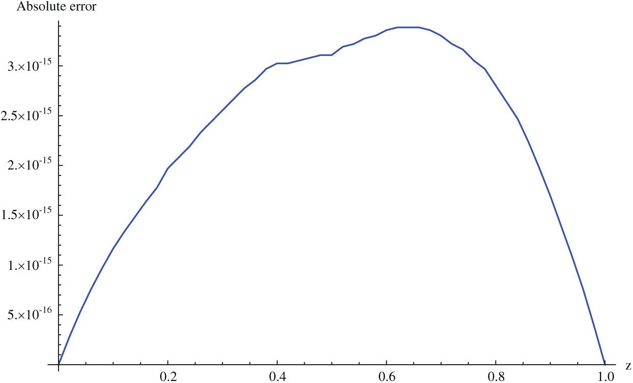
Figure 9: Absolute error for Example 6.3 when M = 100,
Example 6.4
The analytical solution is
The comparison of L2 − norm for Example 6.4 using h = 5,
Table 6: Absolute error norms for Example 6.4 using different values of M and
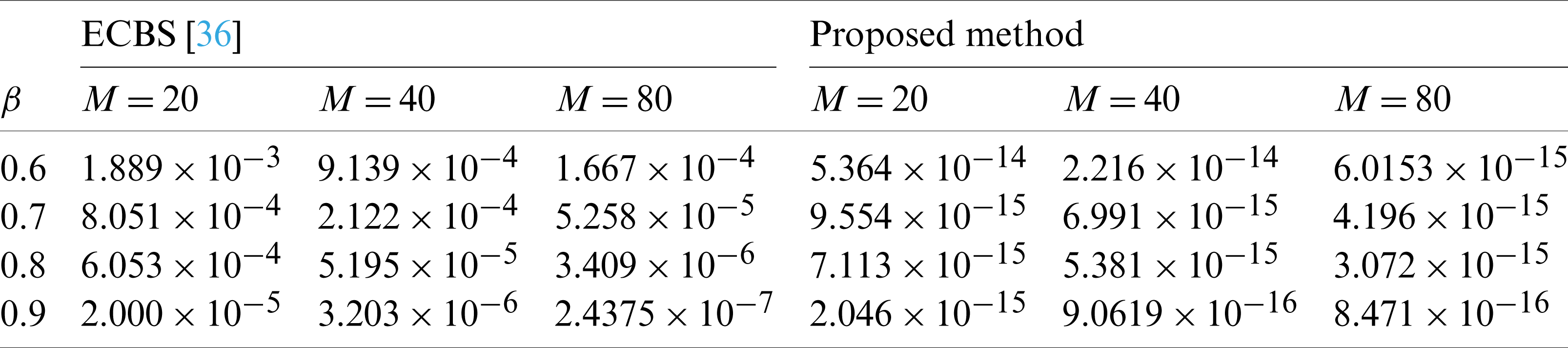
Table 7: Experimental order of convergence for Example 6.4 using different values of M and
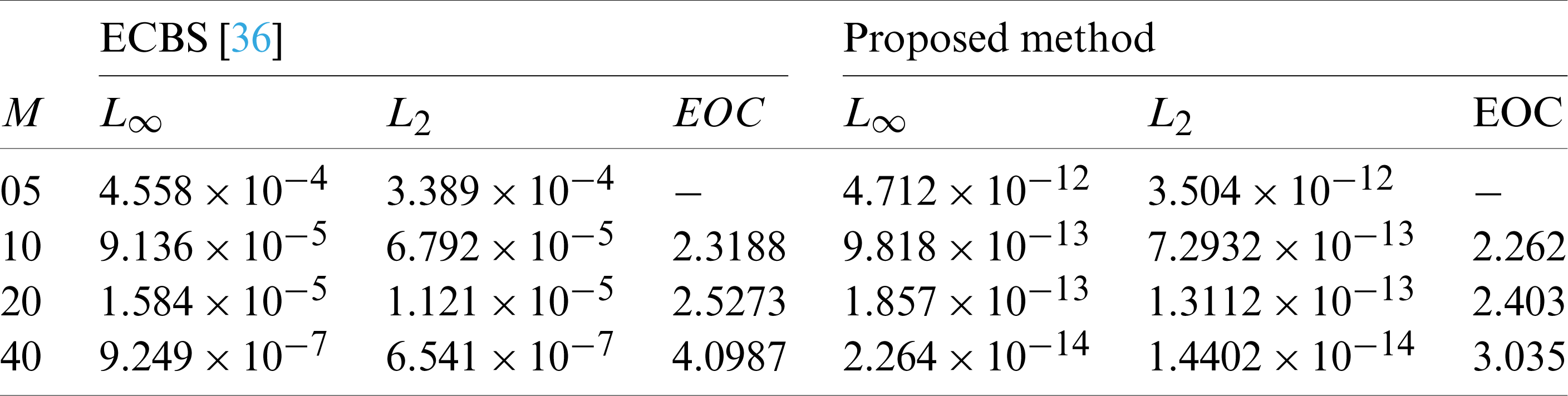
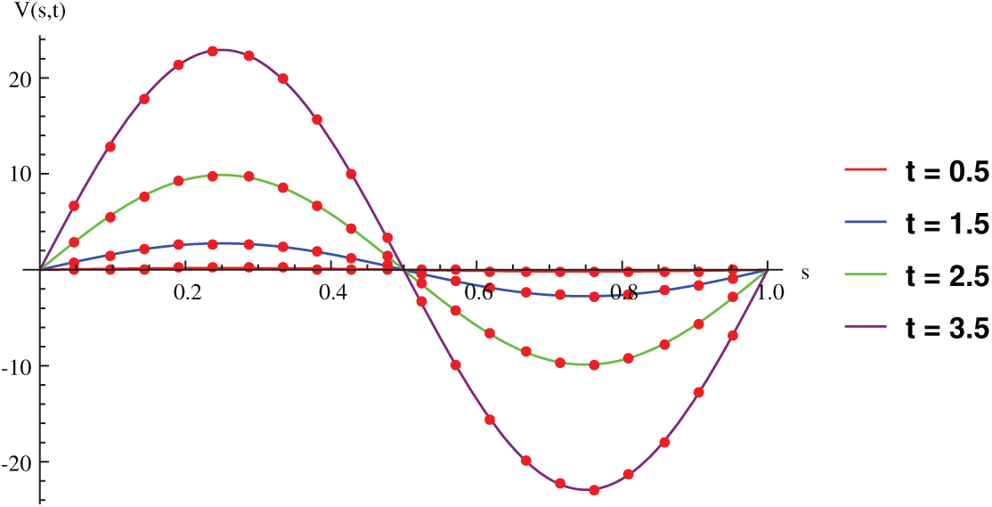
Figure 10: Exact and numerical solution for Example 6.4 at different time levels when
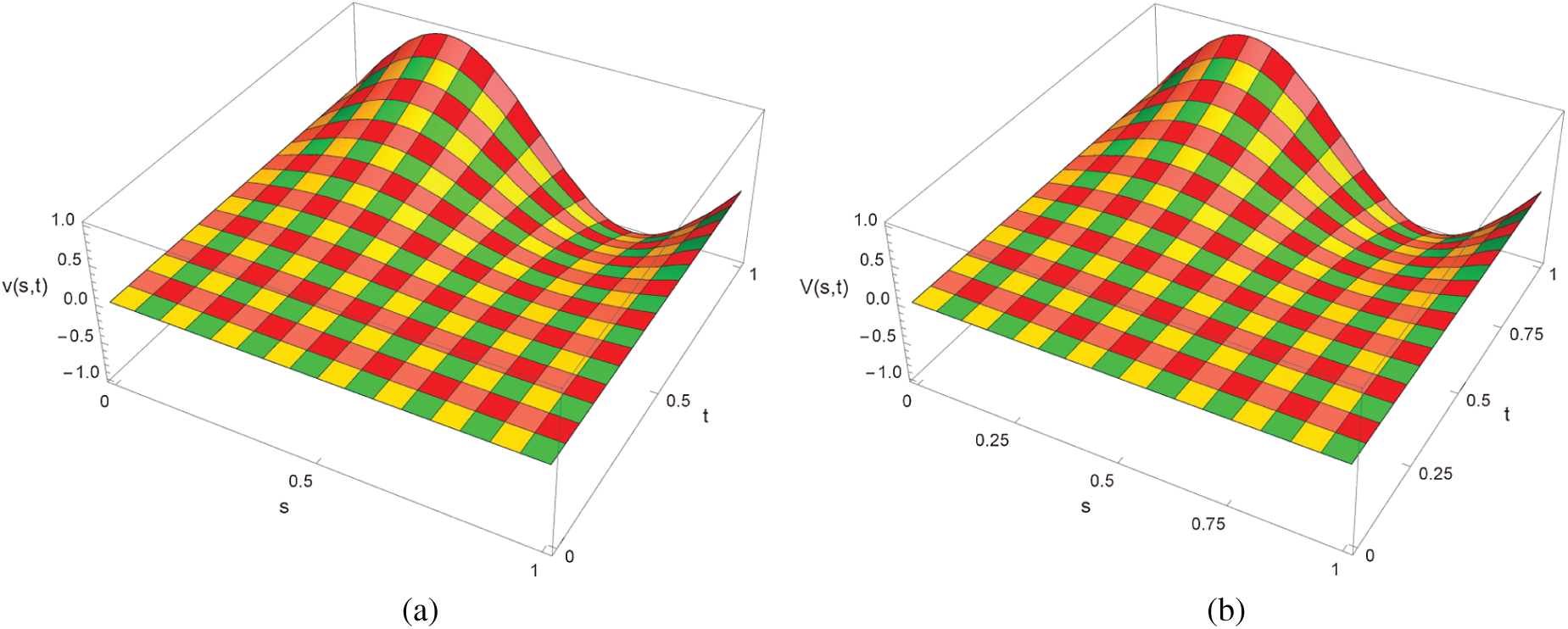
Figure 11: Exact and approximate solution for Example 6.4 with M = 20,
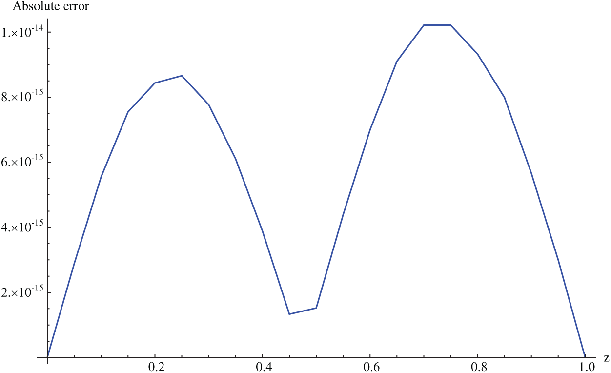
Figure 12: Absolute error for Example 6.4 when M = 20,
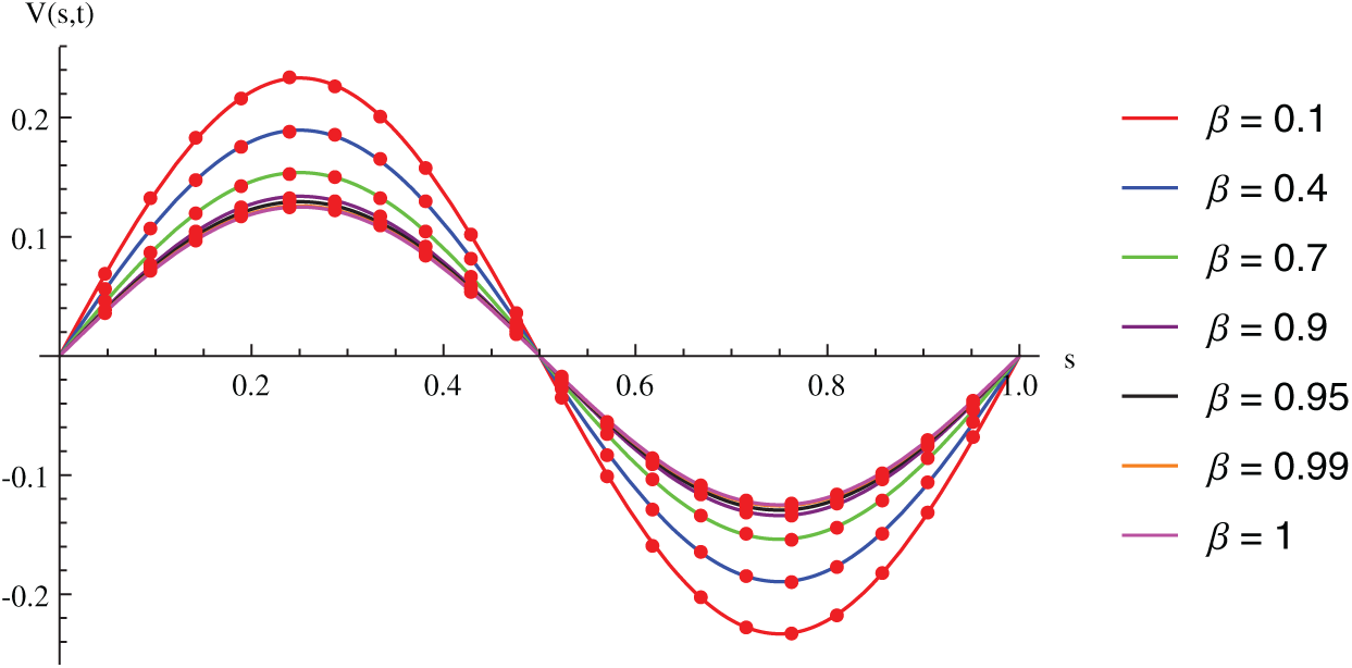
Figure 13: Exact and numerical solutions for Example 6.4 with different values of
This work is concluded with following remarks:
1. An efficient algorithm based on a redefined set extended basis splines is proposed for numerical solution of multi-term time-fractional telegraph equation.
2. The fractional time derivatives have been considered in the Caputo sense.
3. The finite difference formulae have been used to discretize time-fractional derivatives while the discretization of spatial derivatives has been achieved by means of redefined extended B-spline functions.
4. The spatial discretization used in this manuscript is superior to the other existing methods because the proposed method give continuous approximation with high accuracy to the solution curve of the unknown function and its derivatives at each and every point of the range of integration.
5. The stability of presented algorithm has been proved along temporal grid.
6. The theoretical results show that the accuracy of presented numerical approach in spatial direction is of order O(h2) whereas in time direction it is
7. The numerical rate of convergence is in the line with theoretical results.
8. The comparison of error norms reveals that in terms of accuracy and straightforward implementation, the proposed algorithm performs better than the methods in [27,29,30,36].
Acknowledgement: We thank Dr. Nauman Khalid, Govt Post Graduate College, Faisalabad, Pakistan for his assistance in proofreading the manuscript.
Funding Statement: The author(s) received no specific funding for this study.
Conflicts of Interest: The authors declare that they have no conflicts of interest to report regarding the present study.
1. Aguilar, J., Córdova-Fraga, T., Tórres-Jiménez, J., Escobar-Jiménez, R., Olivares-Peregrino, V. et al. (2016). Nonlocal transport processes and the fractional cattaneo-vernotte equation. Mathematical Problems in Engineering, 2016(1), 1–15. DOI 10.1155/2016/7845874. [Google Scholar] [CrossRef]
2. Gómez-Aguilar, J., Escobar-Jiménez, R., López-López, M., Alvarado-Martnez, V. (2016). Atangana-baleanu fractional derivative applied to electromagnetic waves in dielectric media. Journal of Electromagnetic Waves and Applications, 30(15), 1937–1952. DOI 10.1080/09205071.2016.1225521. [Google Scholar] [CrossRef]
3. Atangana, A. (2015). On the stability and convergence of the time-fractional variable order telegraph equation. Journal of Computational Physics, 293(3), 104–114. DOI 10.1016/j.jcp.2014.12.043. [Google Scholar] [CrossRef]
4. Touchent, K. A., Belgacem, F. B. M. (2015). Nonlinear fractional partial differential equations systems solutions through a hybrid homotopy perturbation sumudu transform method. Nonlinear Studies, 22(4), 591–600. [Google Scholar]
5. Atangana, A., Bonyah, E. (2019). Fractional stochastic modeling: New approach to capture more heterogeneity. Chaos: An Interdisciplinary Journal of Nonlinear Science, 29(1), 13118. DOI 10.1063/1.5072790. [Google Scholar] [CrossRef]
6. Riaz, M. B., Atangana, A., Iftikhar, N. (2020). Heat and mass transfer in maxwell fluid in view of local and non-local differential operators. Journal of Thermal Analysis and Calorimetry, 96(1), 1–17. DOI 10.1007/s10973-020-09383-7. [Google Scholar] [CrossRef]
7. Atangana, A., Bonyah, E., Elsadany, A. (2020). A fractional order optimal 4D chaotic financial model with mittag-leffler law. Chinese Journal of Physics, 65(2), 38–53. DOI 10.1016/j.cjph.2020.02.003. [Google Scholar] [CrossRef]
8. Atangana, A., Hammouch, Z. (2019). Fractional calculus with power law: The cradle of our ancestors. European Physical Journal Plus, 134(9), 429. DOI 10.1140/epjp/i2019-12777-8. [Google Scholar] [CrossRef]
9. Owolabi, K. M., Hammouch, Z. (2019). Mathematical modeling and analysis of two-variable system with noninteger-order derivative. Chaos: An Interdisciplinary Journal of Nonlinear Science, 29(1), 13145. DOI 10.1063/1.5086909. [Google Scholar] [CrossRef]
10. Owolabi, K. M., Hammouch, Z. (2019). Spatiotemporal patterns in the Belousov–Zhabotinskii reaction systems with atangana-baleanu fractional order derivative. Physica A: Statistical Mechanics and its Applications, 523(303), 1072–1090. DOI 10.1016/j.physa.2019.04.017. [Google Scholar] [CrossRef]
11. Ghalib, M. M., Zafar, A. A., Hammouch, Z., Riaz, M. B., Shabbir, K. (2020). Analytical results on the unsteady rotational flow of fractional-order non-newtonian fluids with shear stress on the boundary. Discrete & Continuous Dynamical Systems-S, 13(3), 683–693. DOI 10.3934/dcdss.2020037. [Google Scholar] [CrossRef]
12. Uçar, S., Uçar, E., Özdemir, N., Hammouch, Z. (2019). Mathematical analysis and numerical simulation for a smoking model with Atangana–Baleanu derivative. Chaos, Solitons & Fractals, 118, 300–306. DOI 10.1016/j.chaos.2018.12.003. [Google Scholar] [CrossRef]
13. Ullah, S., Khan, M. A., Farooq, M., Hammouch, Z., Baleanu, D. (2019). A fractional model for the dynamics of tuberculosis infection using caputo-fabrizio derivative. Discrete & Continuous Dynamical Systems-S, 13(3), 975–993. DOI 10.3934/dcdss.2020057. [Google Scholar] [CrossRef]
14. Asif, N., Hammouch, Z., Riaz, M., Bulut, H. (2018). Analytical solution of a maxwell fluid with slip effects in view of the caputo-fabrizio derivative. European Physical Journal Plus, 133(7), 272. DOI 10.1140/epjp/i2018-12098-6. [Google Scholar] [CrossRef]
15. Singh, J., Kumar, D., Hammouch, Z., Atangana, A. (2018). A fractional epidemiological model for computer viruses pertaining to a new fractional derivative. Applied Mathematics and Computation, 316(30), 504–515. DOI 10.1016/j.amc.2017.08.048. [Google Scholar] [CrossRef]
16. Weston, V., He, S. (1993). Wave splitting of the telegraph equation in R3 and its application to inverse scattering. Inverse Problems, 9(6), 789–812. DOI 10.1088/0266-5611/9/6/013. [Google Scholar] [CrossRef]
17. Dehghan, M., Shokri, A. (2008). A numerical method for solving the hyperbolic telegraph equation. Numerical Methods for Partial Differential Equations: An International Journal, 24(4), 1080–1093. DOI 10.1002/num.20306. [Google Scholar] [CrossRef]
18. El-Azab, M., El-Gamel, M. (2007). A numerical algorithm for the solution of telegraph equations. Applied Mathematics and Computation, 190(1), 757–764. DOI 10.1016/j.amc.2007.01.091. [Google Scholar] [CrossRef]
19. Momani, S. (2005). Analytic and approximate solutions of the space-and time-fractional telegraph equations. Applied Mathematics and Computation, 170(2), 1126–1134. DOI 10.1016/j.amc.2005.01.009. [Google Scholar] [CrossRef]
20. Dehghan, M., Yousefi, S., Lotfi, A. (2011). The use of He’s variational iteration method for solving the telegraph and fractional telegraph equations. International Journal for Numerical Methods in Biomedical Engineering, 27(2), 219–231. DOI 10.1002/cnm.1293. [Google Scholar] [CrossRef]
21. Das, S., Vishal, K., Gupta, P., Yildirim, A. (2011). An approximate analytical solution of time-fractional telegraph equation. Applied Mathematics and Computation, 217(18), 7405–7411. DOI 10.1016/j.amc.2011.02.030. [Google Scholar] [CrossRef]
22. Hayat, U., Mohyud-Din, S. (2013). Homotopy perturbation technique for time fractional telegraph equations. International Journal of Modern Theoretical Physics, 2(1), 33–41. DOI 10.1080/00207160902874653. [Google Scholar] [CrossRef]
23. Wei, L., Dai, H., Zhang, D., Si, Z. (2014). Fully discrete local discontinuous galerkin method for solving the fractional telegraph equation. Calcolo, 51(1), 175–192. DOI 10.1007/s10092-013-0084-6. [Google Scholar] [CrossRef]
24. Hosseini, V. R., Chen, W., Avazzadeh, Z. (2014). Numerical solution of fractional telegraph equation by using radial basis functions. Engineering Analysis with Boundary Elements, 38, 31–39. DOI 10.1016/j.enganabound.2013.10.009. [Google Scholar] [CrossRef]
25. Srivastava, V. K., Awasthi, M. K., Tamsir, M. (2013). Rdtm solution of caputo time fractional-order hyperbolic telegraph equation. AIP Advances, 3(3), 32142. DOI 10.1063/1.4799548. [Google Scholar] [CrossRef]
26. Wang, J., Zhao, M., Zhang, M., Liu, Y., Li, H. (2014). Numerical analysis of an H1-Galerkin mixed finite element method for time fractional telegraph equation. Scientific World Journal, 2014, 14. DOI 10.1155/2014/371413. [Google Scholar] [CrossRef]
27. Modanli, M., Akgül, A. (2017). Numerical solution of fractional telegraph differential equations by theta-method. European Physical Journal Special Topics, 226(16–18), 3693–3703. DOI 10.1140/epjst/e2018-00088-6. [Google Scholar] [CrossRef]
28. Xu, X., Xu, D. (2018). Legendre wavelets direct method for the numerical solution of time-fractional order telegraph equations. Mediterranean Journal of Mathematics, 15(1), 27. DOI 10.1007/s00009-018-1074-3. [Google Scholar] [CrossRef]
29. Wang, Y., Mei, L. (2017). Generalized finite difference/spectral galerkin approximations for the time-fractional telegraph equation. Advances in Difference Equations, 2017(1), 281. DOI 10.1186/s13662-017-1348-2. [Google Scholar] [CrossRef]
30. Uddin, M., Ali, A. (2018). On the approximation of time-fractional telegraph equations using localized kernel-based method. Advances in Difference Equations, 2018(1), 305. DOI 10.1186/s13662-018-1775-8. [Google Scholar] [CrossRef]
31. Xu, G., Wang, G. Z. (2008). Extended cubic uniform B-spline and α-B-spline. Acta Automatica Sinica, 34(8), 980–984. DOI 10.1016/S1874-1029(08)60047-6. [Google Scholar] [CrossRef]
32. Mohyud-Din, S. T., Akram, T., Abbas, M., Ismail, A. I., Ali, N. H. (2018). A fully implicit finite difference scheme based on extended cubic B-splines for time fractional advection-diffusion equation. Advances in Difference Equations, 2018(1), 109. DOI 10.1186/s13662-018-1537-7. [Google Scholar] [CrossRef]
33. Benson, D. A., Schumer, R., Meerschaert, M. M., Wheatcraft, S. W. (2001). Fractional dispersion, lévy motion, and the made tracer tests. Transport in Porous Media, 42(1–2), 211–240. DOI 10.1023/A:1006733002131. [Google Scholar] [CrossRef]
34. Khalid, N., Abbas, M., Iqbal, M. K., Baleanu, D. (2019). A numerical algorithm based on modified extended B-spline functions for solving time-fractional diffusion wave equation involving reaction and damping terms. Advances in Difference Equations, 2019(1), 378. DOI 10.1186/s13662-019-2318-7. [Google Scholar] [CrossRef]
35. Wasim, I., Abbas, M., Amin, M. (2018). Hybrid B-spline collocation method for solving the generalized burgers-fisher and burgers-huxley equations. Mathematical Problems in Engineering, 2018(10), 1–18. DOI 10.1155/2018/6143934. [Google Scholar] [CrossRef]
36. Akram, T., Abbas, M., Ismail, A. I., Ali, N. H. M., Baleanu, D. (2019). Extended cubic B-splines in the numerical solution of time fractional telegraph equation. Advances in Difference Equations, 2019(1), 365. DOI 10.1186/s13662-019-2296-9. [Google Scholar] [CrossRef]
 | This work is licensed under a Creative Commons Attribution 4.0 International License, which permits unrestricted use, distribution, and reproduction in any medium, provided the original work is properly cited. |