| Computer Modeling in Engineering & Sciences |
DOI: 10.32604/cmes.2021.013632
ARTICLE
Three-Dimensional Modeling of the Retinal Vascular Tree via Fractal Interpolation
1Electronics and Microelectronics Laboratory, Department of Physics, Faculty of Sciences, Monastir University, Monastir, 5019, Tunisia
2Department of Computer Science and Information, College of Science, Majmaah University, Zulfi, 11932, Saudi Arabia
3Department of Physics, College of Science Zulfi, Majmaah University, Zulfi, 11932, Saudi Arabia
*Corresponding Author: Hichem Guedri. Email: Hichem.Guedri@fsm.rnu.tn
Received: 14 August 2020; Accepted: 21 December 2020
Abstract: In recent years, the three dimensional reconstruction of vascular structures in the field of medical research has been extensively developed. Several studies describe the various numerical methods to numerical modeling of vascular structures in near-reality. However, the current approaches remain too expensive in terms of storage capacity. Therefore, it is necessary to find the right balance between the relevance of information and storage space. This article adopts two sets of human retinal blood vessel data in 3D to proceed with data reduction in the first part and then via 3D fractal reconstruction, recreate them in a second part. The results show that the reduction rate obtained is between 66% and 95% as a function of the tolerance rate. Depending on the number of iterations used, the 3D blood vessel model is successful at reconstruction with an average error of 0.19 to 5.73 percent between the original picture and the reconstructed image.
Keywords: Fractal interpolation; 3D Douglas–Peucker algorithm; 3D skeleton; blood vessel tree; iterated function system; retinal image
The three-dimensional reconstruction of vascular structures has major medical significance in the diagnosis and prognosis of several diseases, including atheromatous disorders [1]. The downside of three-dimensional reconstruction methods is they are too expensive in terms of storage capacity and transmission time [2–11].
The preliminary step to describe images or curves is the extraction of the interest regions. There are many detectors of interest points and interest regions whose purpose is to extract points or regions that have particular properties [12–20] (corners, outlines, projecting regions, etc.) and which are stable in acquisition conditions variations.
This study focused on the description of the regions provided by the Douglas–Peucker 3D procedure. The advantage of this constraint is to cancel all unnecessary geometric invariance of the descriptor in order to increase its discriminating power [21–27].
The aim of this study is to develop a technique that enables a large amount of data to be produced with few errors and very little information to be used as input.
In order to achieve the goal, a novel mathematical morphology-based technique is proposed to ensure a 3D reconstruction taking the entire problem into account.
This study interested in the reconstruction of the 3D skeletons of the blood vessels by the fractal technique. Beginning with a 3D model is based on an approximation of the actual topology of the human retina vascular trees. In the first step, the 3D thinning algorithm presented to detect the blood vessel centerline [12–16]. Thereafter, the crossing number techniques are used to extract the characteristic points [17–20]. Define the characteristic points using the Douglas–Peucker 3D algorithm represent the next step [21–27]. In the final critical step, the 3D Fractal Interpolation and IFS (iterated function systems) algorithm is implemented for 3D reconstruction [28–35].
Several methodologies have been developed in the literature for the reconstruction of a 3D model based on the fractal method. Several 3D fractal algorithms are available. Xiong et al. [29] has proposed a method based on 3D fractal interpolation to reconstruct the 3D terrain surface. This technique uses the fractional Brownian motion (fBm) model to interpolate the surface of this surface. Guedri et al. [30] have used fractal 3D and IFS 3D interpolation to reconstruct a 3D blood vessels model. The flowchart of their proposed algorithm: It consists of two main stages; Stage 1 for detection of the characteristic points by using the 2D Douglas–Peucker (DP) method, and subsequently, in Stage 2, more data points were added using random fractal interpolation approach, to reconstruct a three-dimensional (3D) model of the blood vessel. He et al. [31] have proposed a method to accelerate the execution of probability-based fractal interpolation. They have used the fractal interpolation to reconstruct 3D topography using a little scattered point in the Digital Elevation Model (DEM). Li et al. [32] have presented algorithms for estimating the fractal dimension and the texture gap as fractal characters. An improved subdivision scheme has been developed to reconstruct the fractal surface from extracted fractal characters. They have combined the demonstration of characterization and fractal reconstruction for irregularly measured geochemical data from 1767 stream sediment samples. Guo et al. [33] have proposed a method that combines the fractal dimension and the Marching Cubes algorithm to reconstruct a three-dimensional internal tissue model. They have used fractal interpolation to obtain detailed information on internal tissues. This 3D model of internal tissues is displayed using the Visualization Toolkit (VTK) software. Huang et al. [34] have used the 3D fractal technique to reconstruct two real-world 3D field data sets. They sampled data randomly and rebuilt it them by 3D fractal reconstruction. Guedri et al. [35] have proposed a 3D fractal technique to reconstruct the cylindrical form of blood vessels. They used the Douglas–Peucker 2D algorithm to detect control points. Then, they used 3D fractal interpolation and iterated function systems for reconstruction the cylindrical shaped of blood vessel.
Fig. 1 demonstrates the algorithms used in this work. There are two main steps: The process of extraction of the 3D blood vessels centerline followed by the process of 3D reconstruction of the blood vessels skeleton by the fractal technique. In a first step, the human retina images contain real information that can be digitally processed to obtain 3D organs models. To be used with confidence, these 3D models must be true to reality. The detection phase of the blood vessel curve is introduced in the next step. Then, 3D skeletal reconstruction of these vessels is performed. Thereafter, this study interested in the defining of distinguishing points based on the Douglas–Peucker procedure. In the final step, 3D Fractal and Iterated Function Systems (IFS) used to visualize and reconstruct the vessels in 3D.
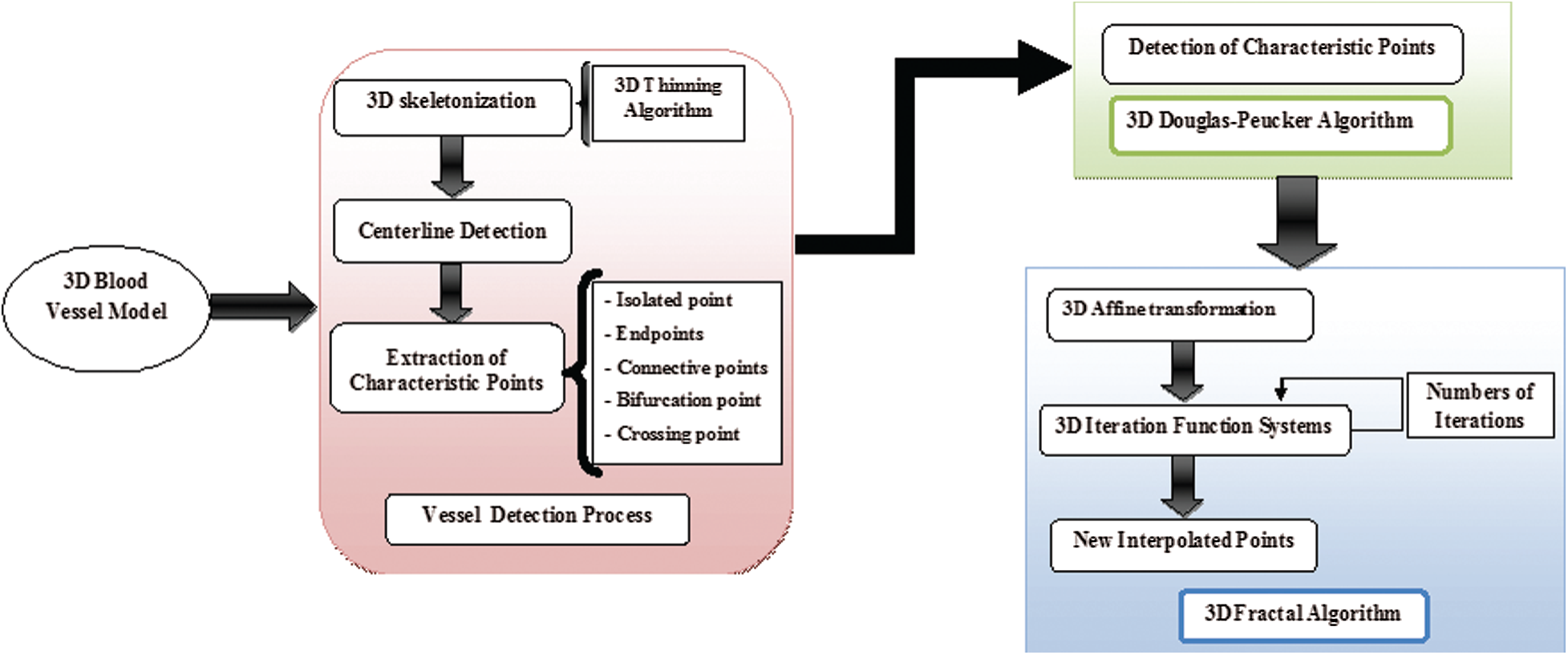
Figure 1: Synoptic flowchart of the proposed 3D fractal reconstruction method
3 Reconstruction of Three-Dimensional Blood Vessel Centerline Network
In recent years, 3D vessel reconstruction has been widely developed in the medical field to allow physicians to diagnose correctly. Several studies describe various numerical approaches to reconstruction of a blood vessel model that is nearest to reality. This section seeks to reconstruct 3D retinal blood vessels image, even when data are missing. The chosen technique allows an optimized the 3D blood vessels reconstruction of is a method related to that offered by Hichem et al. [3].
In the following sections, the results obtained with this procedure are used to obtain the 3D blood vessels centerline.
3.2 Reconstruction of 3D Skeleton
The 3D centerline is measured by an arbitrary 3D volume. It is a 3D thinning procedure implementation. This algorithm is used to detect centerline on images of tubular or filamentous structures. The skeleton must be thin 1-voxel, it must also be fixed for many effects such as shift zoom and rotation, which means that the geometric and topological characterization of the obtained skeleton is invariant when the 3D model is shifted, scaled or rotated [12–15].
In this section, a 3D thinning algorithm is applied to extract the 3D blood vessel centerlines. The complete description of the proposed algorithm has been published in the studies of Palágyi et al. [16].
A 3D thinning algorithm was used which has a directional strategy, there are 4 direction (South, East, North and West) and each direction has three stages (central, up and Down), which gives us generally 12 direction, as shown in Fig. 2. In the proposed approach, every iteration stage involves 12 parallel operations centered on 12 directions. The thinning Algorithm eliminates the border points in 12 iteration steps and repeats the process until no border points have been removed.
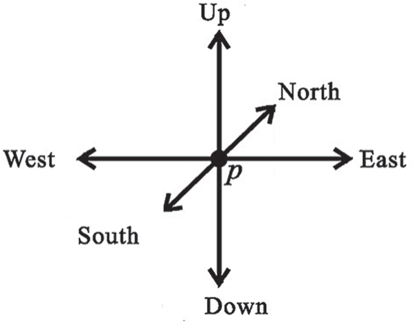
Figure 2: All main directions in 3D
3.3 Characteristic Point’s Extraction
The characteristic points are obtained from the thinned image.
A crossing number is generated for each pixel by an image scan. The Crossing Number CN(p) of a point P
where P
—If
—If
—If
—If
—If
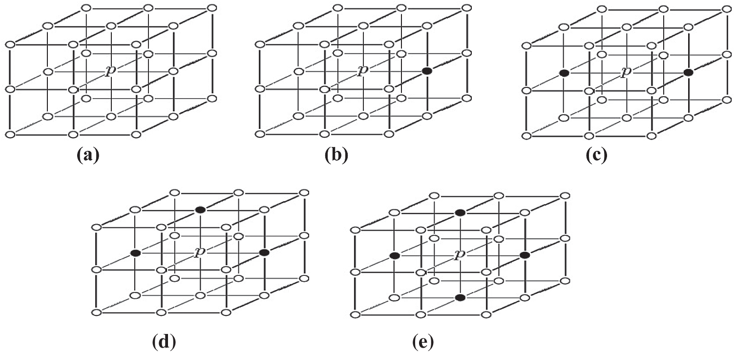
Figure 3: Determination of the different types of pixels in the skeleton image by crossing number algorithm (P: Test pixel, ‘1’: Black pixels, ‘0’: White pixels). (a) Example of isolated pixel (
Fig. 4 shows the example of this characteristics points extraction stage, where the endpoints, the bifurcation points and the central points.
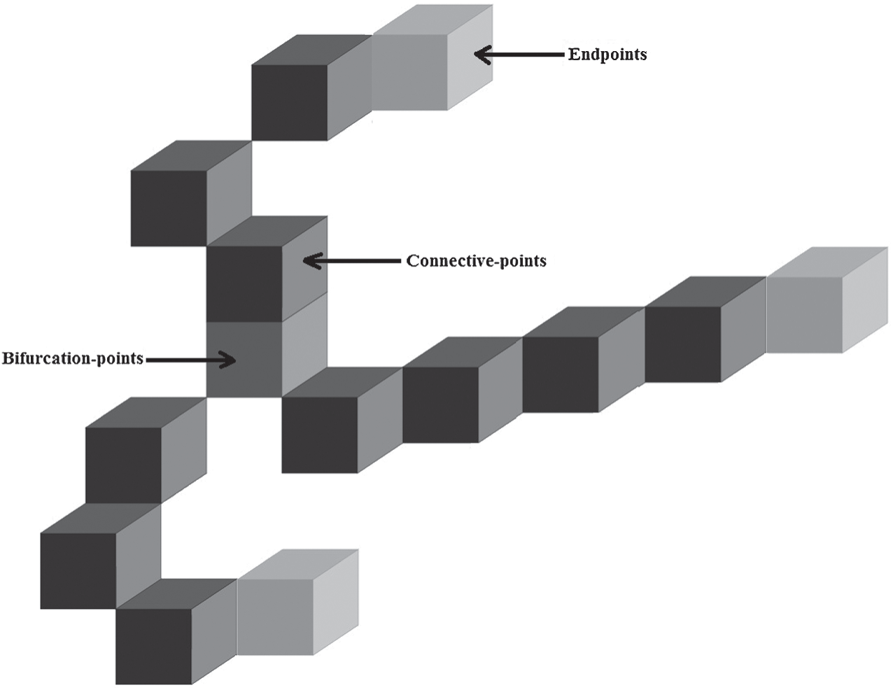
Figure 4: The characteristics points’ extraction
4 The 3D Douglas–Peucker Algorithm
The purpose of simplifying the curve in 2D or 3D is to decrease the number of points needed to represent the curve without changing its main features. The proposed technique of the characteristic point detection is illustrated in the following order [21–27]:
(a) A common origin point O, an anchor point (P) and a floating point (T) are determined to generate an initial basic plane. In this example, the coordinate point designated (
(b) The orthogonal distances between each 3D curve data point and the initial base plane are calculated, as shown in Fig. 5.
(c) If the maximum distance (MD) is less than the predefined threshold (
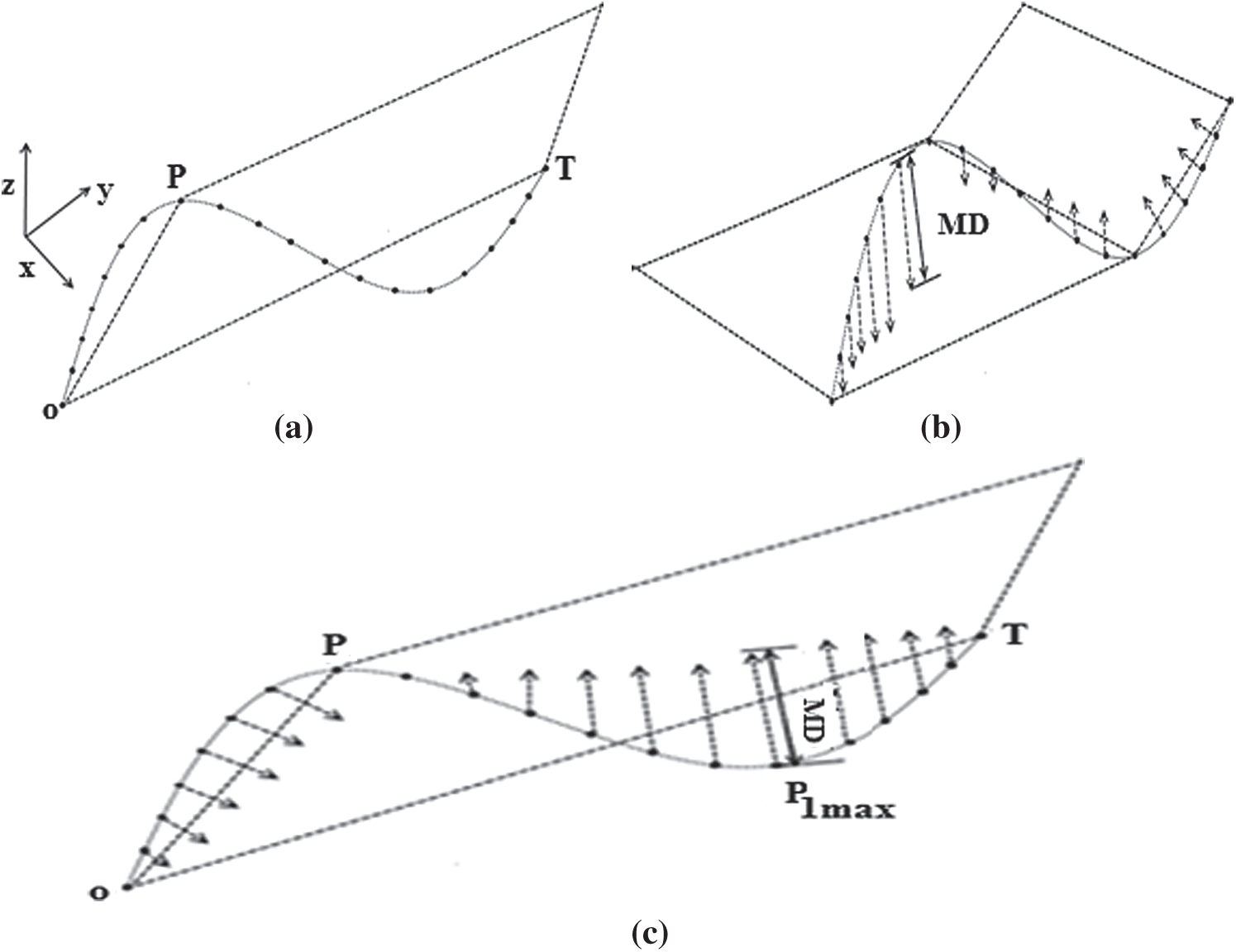
Figure 5: The 3D Douglas–Peucker method, (a) Generation of an initial basic plane, (b) Calculate the orthogonal distances, (c) Division of the 3D curve into two 3D sub-curves
The simplification rate is calculated by:
where I and
Indeed, by detecting regions of interest in images or curves, existing transformations between two regions, which represent the same surface elements, can be modeled by a rotation, a translation and a scaling.
Fractal geometry is a compact description of irregular objects where the use of Euclidean geometry becomes impossible. High complexity of the image, low content of knowledge, fractionality and self-similarity are characterized by fractal objects. They are extremely redundant, consisting of transformed versions of themselves or parts of themselves. Fractal interpolation is based on the modeling of a real-world curve or signal as a fractal object and on the exploitation of the redundancy and self-similarity appears in the fractal objects according to the iteration function systems (IFS). IFS are affine transformations set 3D [28–35] or 2D [36–41] combining rotation, scaling and translation at the same time.
This study presents the development of iterated functions systems for the reconstruction of the 3D skeleton.
5.1.1 2D Affine Transformation
Affine transformation transformations will map points in one space to another point. It combines many operations like Scaling, Rotation, Reflection and Shearing [28–30]. It can express as a single matrix multiplication (A) and a vector addition (T).
Let
Consider the IFS {[x0, x
It is usually written as a system of linear equations [29]:
Here (x, y) are the coordinates of the original curve, and (x
5.1.2 3D Affine Transformations
Consider the interpolation points in 3 dimensions
Let
The 3D transformation is defined by two matrices a diagonal
The 3D affine transformation used in this algorithm is defined as follows:
where (x, y, z) are the coordinates of the 3D original curve and (x
To estimate a solution of the equation, a resolution method proposed based on the division of the initial space (3D) into two sub-spaces 2D (XY) and (XZ). Where the first space (XY) could be modeled by the following transformation
Firstly, the IFS introduce in a 2D (xy) space. A 2D affine transformation consists of two parameters A and T. The y-axis has no rotation term, therefore, the parameter bi = 0 in Eqs. (3) and (4), the coefficients of the
It is represented as [29]:
Then, the same process repeated to the space x-z. For this, the coefficients of the
From this pseudo-division and both Eqs. (6) and (7), the different parameters of the 3D affine transformation were determined, that allows the passage from the origin space to the destination space. Hence the solution to the system is:
where Fractal dimension (DF), estimated by box-counting algorithm [42,43].
As shown in the section above, exploiting the control points, fractal interpolation functions generated, as shown in Fig. 6.
Figure 6: Exploiting the parameters of the fractal interpolation
These parameters are used to generate new interpolated points. The iteration operation started from the initial point P0, the initial point and the affine transforms set are used to create the initial points set. Then, this first points set used and the same affine transforms to create the next points set [38,41].
The same principle continues applied until the generated data point meets the user’s requirements as shown in the following Fig. 7:
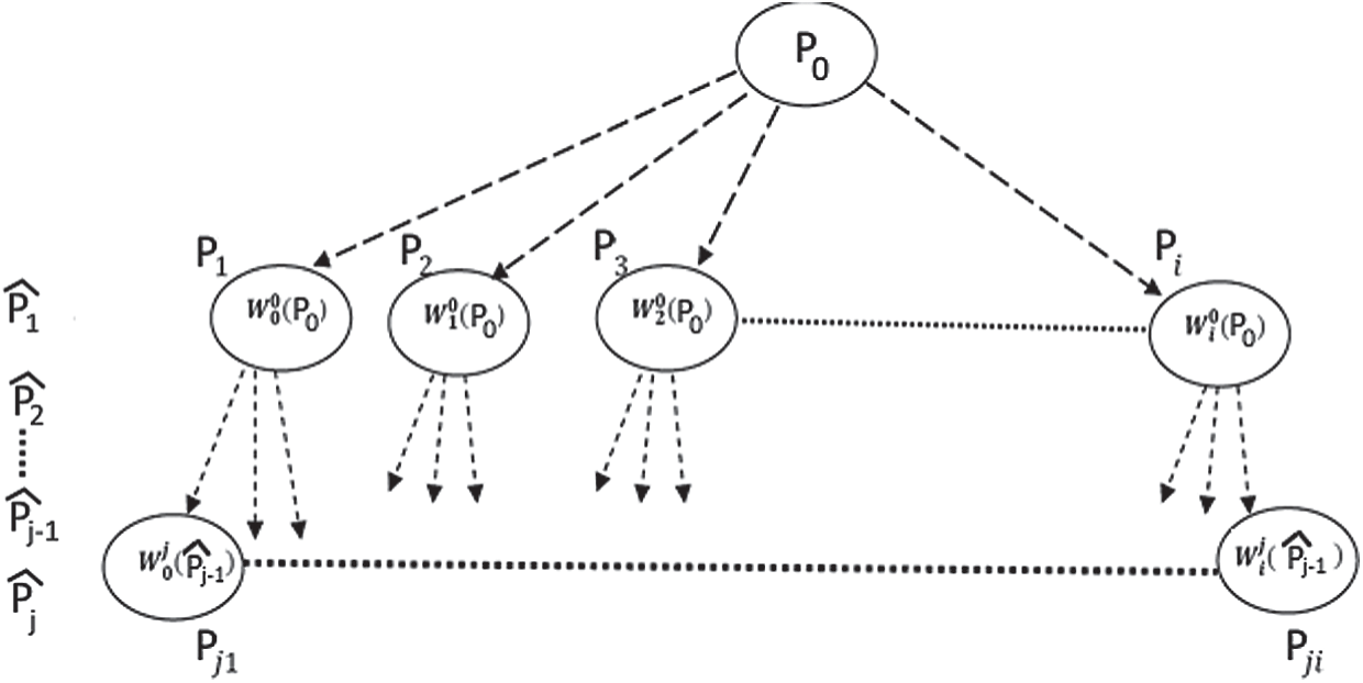
Figure 7: Generation of new 3D points based on fractal interpolation
In order to evaluate proposed method, the test had been coded in Matlab, The program test had been run on a workstation provided with an Intel Pentium processor B960 CPU@2.20 GHz and 4 GB RAM and the proposed algorithm applied on images from two database.
Several databases of retinal images are available. The Digital Retinal Images for Optical Nerve Segmentation Database (DRIONS) [44] are also the most popular databases for vessel segmentation containing low-resolution images, STructured Analysis of the Retina (STARE) [45] and Digital Retinal Images for Vessel Extraction (DRIVE) [46]. Alternatively, other databases such as ADCIS: A Team of Imaging Experts [47] is available, Retinal Identification Database (RIDB) [48], Glaucoma Database Glaucoma (DB) [49] and High-Resolution Fundus (HRF) with higher resolutions [50]. During this study, the images illustrated from the database STARE and HRF, to test whether the resolution of the image used has an influence on the reconstruction error.
6.1.1 High-Resolution Fundus (HRF)
The database had three image sets: Each set had 15 images, first set for normal, second set for patients with diabetic retinopathy and third one for glaucomatous patients. All images are taken with a fundus camera CANON CF-60 UVi outfitted with CANON EOS-20D digital cameras, the capture angle with a field of view of 45
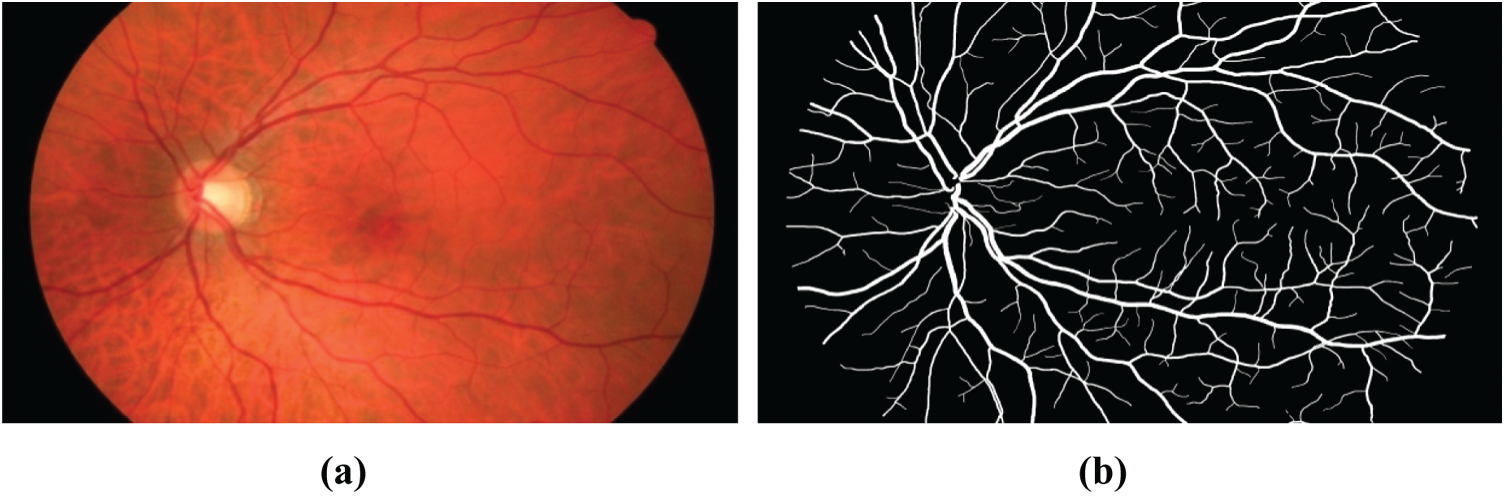
Figure 8: Fundus image of the high-resolution fundus (HRF) database: (a) Raw image, (b) Manual blood vessel segmentation
6.1.2 STructured Analysis of the Retina (STARE)
In this database, there are twenty retinal fundus images with ten of them have pathologies. The images were captured by a TopCon TRV-50 fundus camera at 35
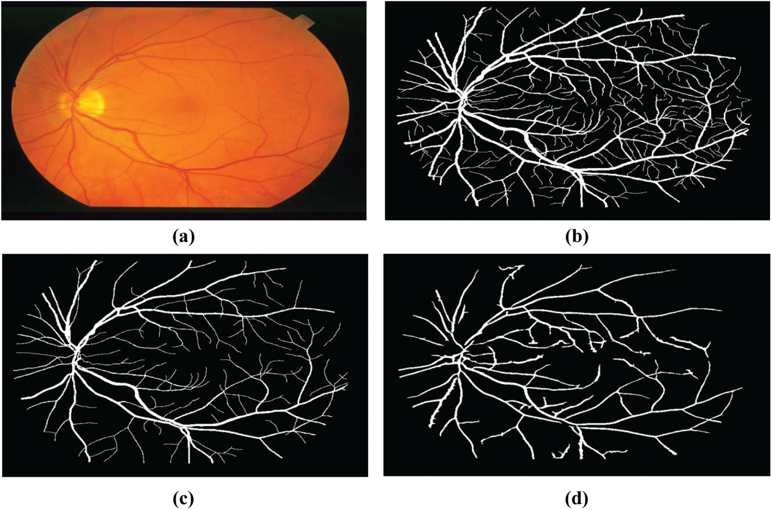
Figure 9: Example fundus image of the structured analysis of the Retina (STARE), (a) Raw image im0162.jpg, (b, c) Their respective manual segmentation, (d) Segmentation results created by matched spatial filter probing algorithm
The proposed technique by Hichem et al. [3] was applied, to reconstruct 3D blood vessels from retinal images. The result of the 3D retinal blood vessels model of this algorithm is shown in Fig. 10.
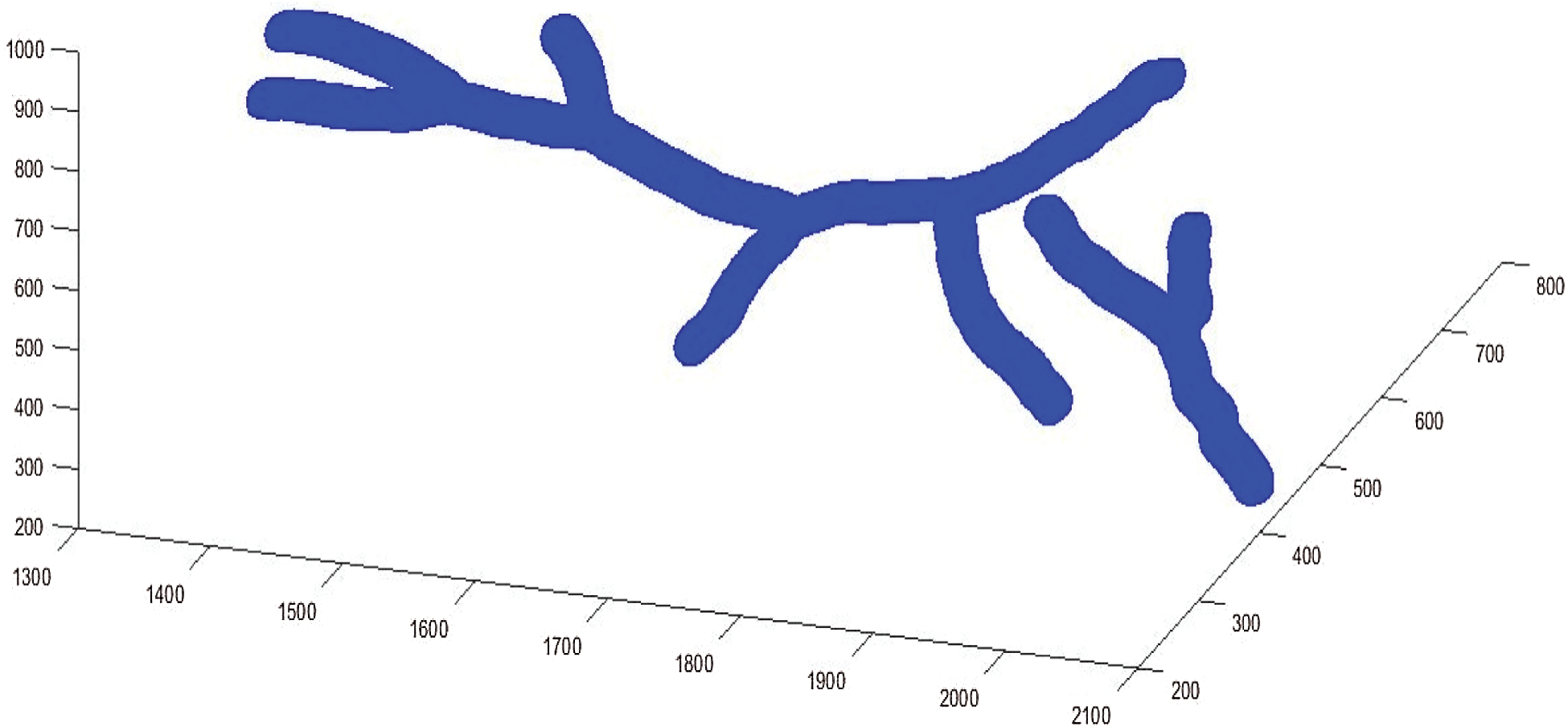
Figure 10: 3D models reconstructed
6.2 3D Skeletons Reconstruction
After getting the 3D model, the 3D thinning algorithm was used, it is then possible to retain geometric characteristics, the result is called 3D skeleton. These results are given in Fig. 11.
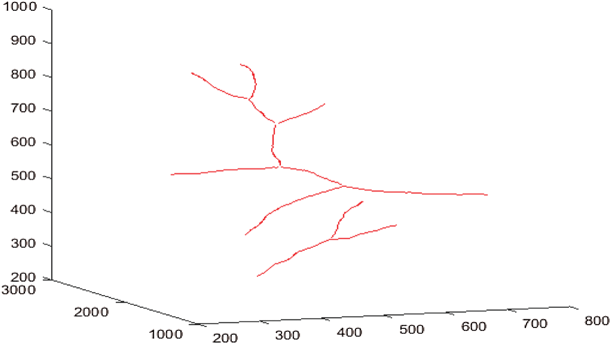
Figure 11: 3D models reconstructed
Fig. 11 shows the experimental results tests by applying the suggested method to segment the blood vessels from image 02_h.jpg and im0162.ah.jpg with different arc length (from 50 to 385 pixels). After performing the 3D skeleton reconstruction of the human retina, the approach we have adopted in this work consists to use the properties of curves simplified by the Douglas–Peucker algorithm.
To evaluate the implemented algorithm, some results will present for the simplification of the 3D blood vessels curve from the centerline of the human retina.
By analyzing the 3D skeleton obtained, it could be noted that the voxel corresponding to the characteristic points have a crossing-number different from 2.
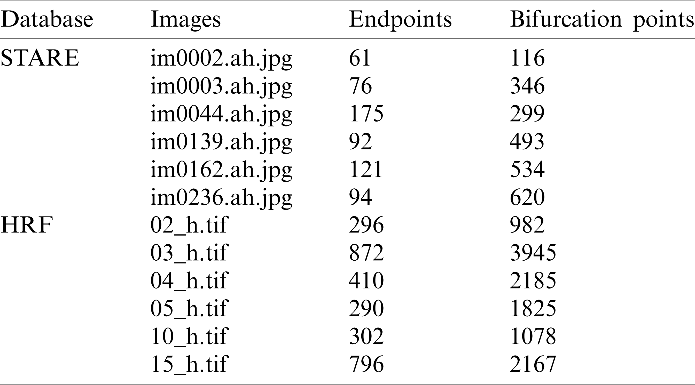
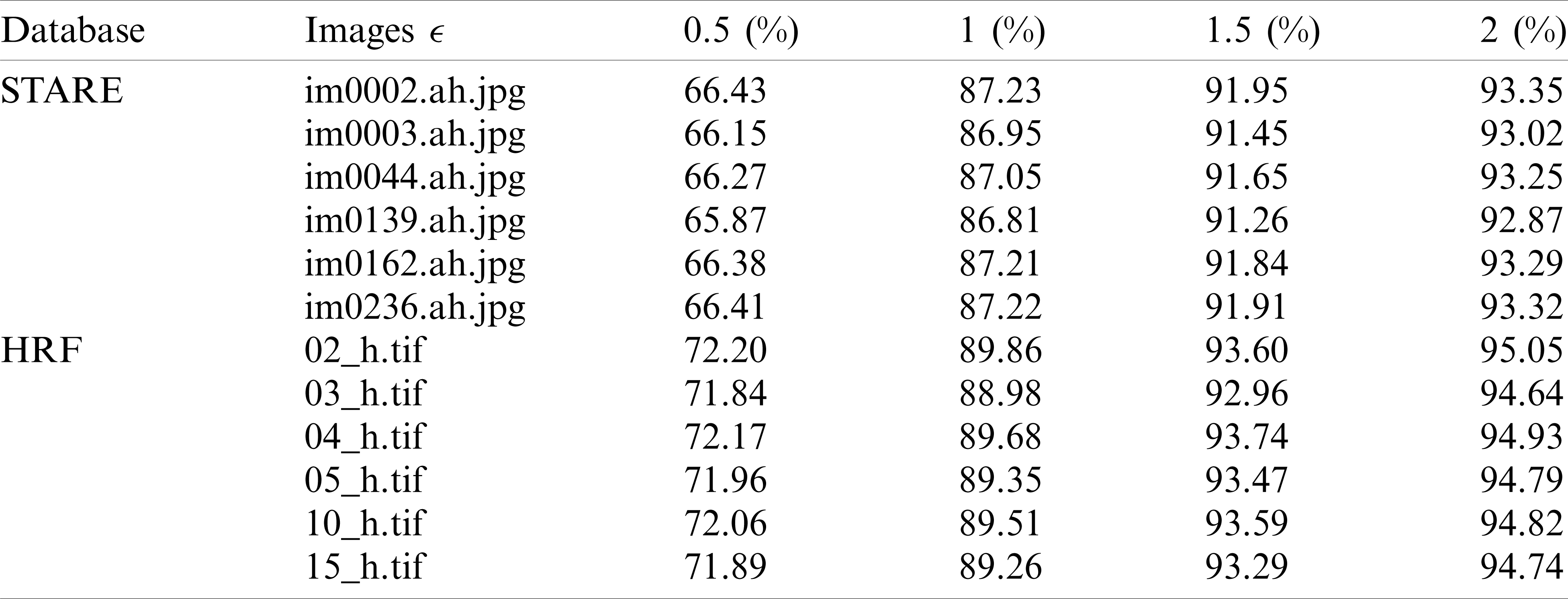
Tab. 1 show several typical results of endpoints and bifurcation point recognition for 6 test images, 3 images from STARE database and 3 images from HRF database. Based on the results, the HRF database sample images received more endpoints and the bifurcations than the images from the remaining database. This is due to the image quality and the appearance in these images of a greater number of blood vessels.
Table 1: Detection of endpoints and bifurcation points for an image from High Resolution Image Database (HRF) and image from STARE database
Figs. 12a–12d shows respectively the simplifications with a tolerance of 0.5, 1, 1.5 and 2 pixels of the 3D blood vessel curve by the Douglas–Peucke algorithm. In red color, it appears the 3D blood vessels curve. In addition, the characteristic points that will be stored and which will be used in the fractal interpolation are in blue.
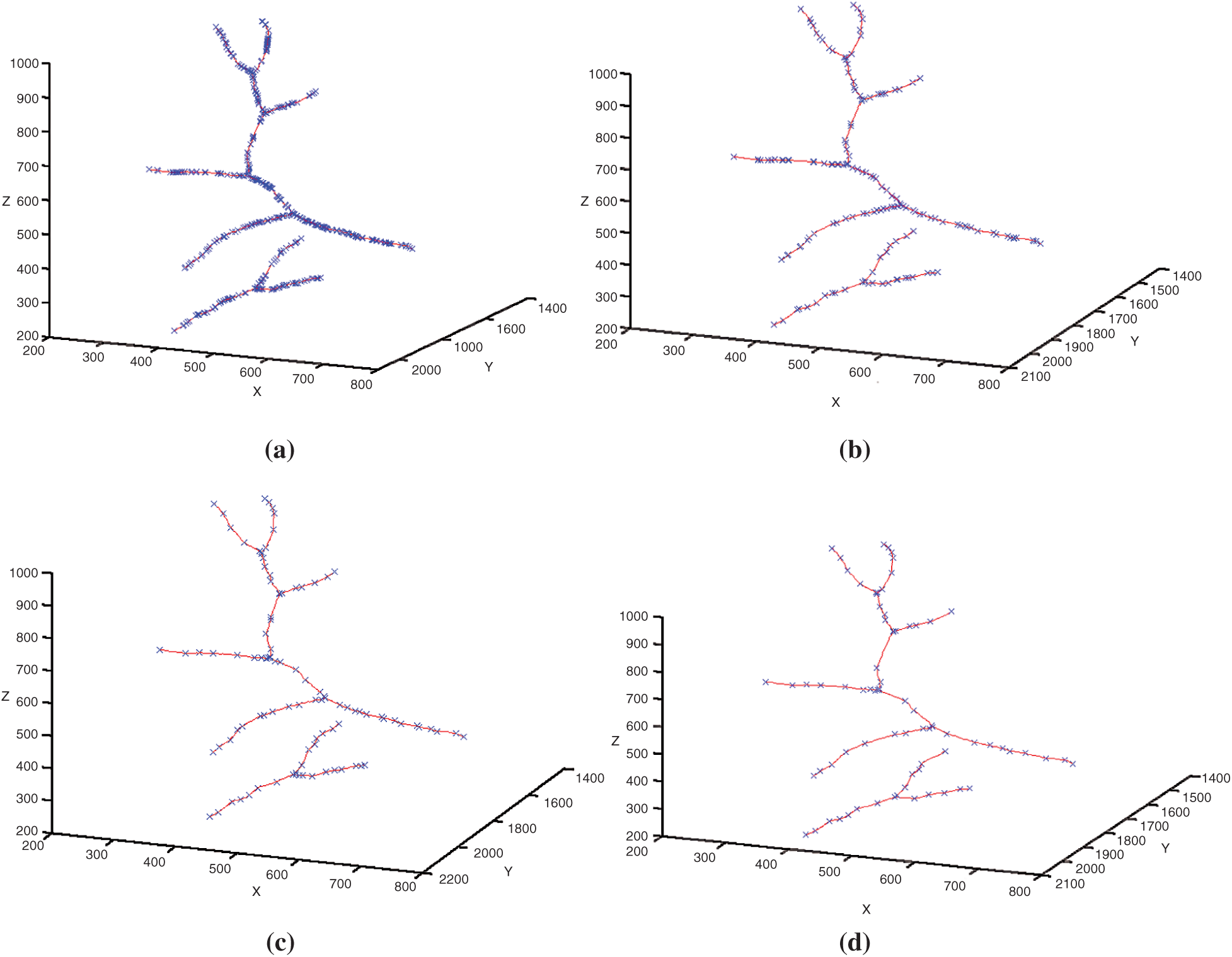
Figure 12: Simplifications of the 3D blood vessel curve by the Douglas–Peucker algorithm for different values of
Tab. 2 reviews the results obtained by the Douglas–Peucker procedure. The oversimplification tolerance is given in column ‘
Table 2: The simplification rate for different tolerance values
The findings in Tab. 2 show that the simplification rate is more than 66 percent and can go up to 95 percent. This simplification rate grows in proportion to the tolerance value ‘
6.4 Reconstruction of the 3D Blood Vessels Skeleton by the Technique Fractal Interpolation
In fact, the results of the Douglas–Peucker algorithm are used first to calculate the different coefficients of the affine transformations matrices Wn. The technique introduced in Section 5 was applied to the 3D blood vessel skeleton curve, and the resulting approximations are shown in Fig. 13.
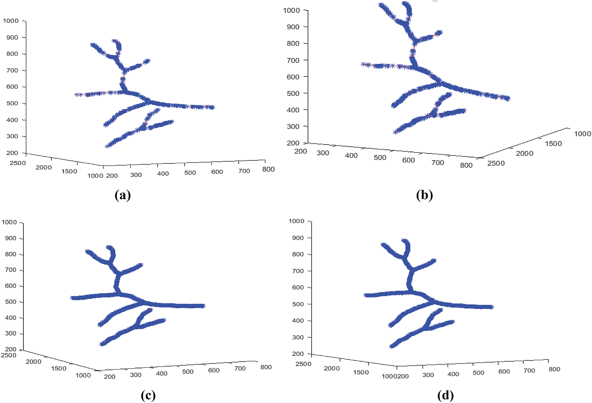
Figure 13: 3D models reconstructed at different iteration numbers N. (a) For
Fig. 13 shows the pseudo-continuous evolution of the 3D models reconstituted after IFS interpolation of the 3D blood vessels curves. The limit case appears for the iterations
In addition, the error rate between the original and the interpolated image in equations is estimated for the study of the efficiency of our interpolation algorithm (8):
If the number of wrong pixels is the number of pixels that do not appear in the interpolated image and the total pixel number is the number of the original image pixels.
The error rate for different iterations numbers N is presented in Figs. 14a, 14b. These two figures show how the quality of the reconstructed images is successively improved by increasing the number of iterations. The results reveal that the error rate is about 5% if the number of iterations
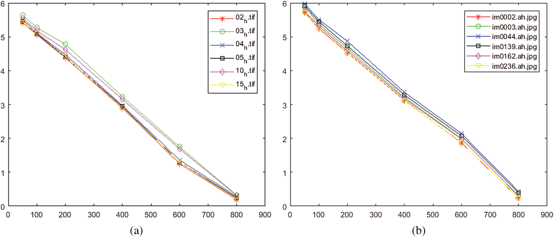
Figure 14: Performance of the proposed method for different numbers of iterations. (a) For test set from HRF database, (b) For test set from STARE database
In this paper, two steps are discussed in the visualization and reconstruction the 3D blood vessels centerlines, using the fractal technique. The first one is carried out for the determination of the characteristic points of the 3D curve of the vascular network, while the second step is carried out for the 3D fractal reconstruction.
As for the first problem, the determination of the characteristic points by the use of the Douglas–Peucker algorithm was studied. Numerous studies have shown that this algorithm has the best rate of data reduction. In a previous work, the numerical results achieved in this study are compared to the values derived from literature formulations. The drop rate of the 2D NEM (numerical elevation model) data profile obtained by the Douglas–Peucker linear simplification method (DP) in the research of Chen et al. [41] is between 50% and 99%. The result obtained by Guedri et al. [30] offers a reduction in the blood vessel curve that is between 78% and 96%. With regard to the structure of the reduction rates, the difference between the above data and the test data in Tab. 2 is between 4 and 10%. It is due to the large difference in asymmetry coefficient. In terms of data point reduction skills, the DP method gives a fast reduction with a high reduction rate. The results obtained show that using the Douglas–Peucker algorithm allows reducing the storage memory of the 3D blood vessels images and reducing costs and transmission time.
Concerning the evolution of 3D fractal reconstruction, the results obtained by Guedri et al. [30] offers an innovative approach for 3D fractal reconstruction with an error between 0.8% and 8%. The method proposed in this research is indeed better in terms of error. The error value is between 0.19% and 5.7%. It is noted that our proposed method can correctly follow all the 3D branches of the blood vessels while having a minimal error.
The advantage of fractal interpolation that it can give points interpolated more than those initially observed. It allows determining the interconnection between these points, so that the 3D curve of the reconstructed blood vessels gets more natural details and more real. However, it requires specialized equipment such as Calculating Unit and digital signal processor (DSP) due to the computational complexity in the algorithm.
In this study, a 3D model of a tree of retinal blood vessels presented, reconstructed from a fundus image using the fractal technique and IFS 3D, also a 3D model of a tree of retinal blood vessels, reconstructed from a fundus image using the fractal technique and IFS 3D. First, a 3D model relies on an approximation of the real topology of the human retina vascular trees. In the first part, the 3D thinning algorithm is used to detect the blood vessel centerline (3D skeleton). Then, the characteristic points are extracted from the curve of centerline obtained. The next step illustrated the use of Douglas–Peucker 3D algorithm to determine the characteristic points. The reduction rate obtained to maintain the whole structure of the vascular tree is between 66% and 95% as a function of the tolerance value. It is found that the reduction rate is relatively higher in the case of a larger tolerance value. Finally, a 3D fractal descriptor and 3D IFS algorithm were used for 3D fractal reconstruction. The results obtained showed that the error committed between the original image and the reconstructed image is between 0.19% and 5.73%. As well as, the interpolated data points gave a higher resolution than the original model. On the other hand, the reconstructed 3D models have an almost real and natural appearance with more detailed characteristics with a higher resolution than initially observed.
Funding Statement: The author(s) received no specific funding for this study.
Conflicts of Interest: The authors declare that they have no conflicts of interest to report regarding the present study.
1. Abdeljabbar, G., lbrahim, A. A. (2019). An analytical study on the fractional transient heating within the skin tissue during the thermal therapy. Journal of Thermal Biology, 82, 229–233. DOI 10.1016/j.jtherbio.2019.04.003. [Google Scholar] [CrossRef]
2. Yu, M., Meng, H., Liu, G. Z. (2018). 3D reconstruction of fundus vascular structure based on binocular stereovision. 4th Annual International Conference on Network and Information Systems for Computers, pp. 140–143. Wuhan, China. [Google Scholar]
3. Hichem, G., Chouchene, F., Belmabrouk, H. (2015). 3D model reconstruction of blood vessels in the retina with tubular structure. International Journal on Electrical Engineering and Informatics, 7, 724–773. DOI 10.15676/ijeei.2015.7.4.14. [Google Scholar] [CrossRef]
4. Zhao, Y. T., Xie, J. Y., Zhang, H. Z., Zheng, Y. L., Zhao, Y. F. et al. (2020). Retinal vascular network topology reconstruction and artery/vein classification via dominant set clustering. IEEE Transactions on Medical Imaging, 39(2), 341–356. DOI 10.1109/TMI.2019.2926492. [Google Scholar] [CrossRef]
5. Son, J. W., Lee, W. S., Lee, S. J., Choi, Y. (2017). Accurate three-dimensional modeling of blood vessels using computer tomography, intravascular ultrasound, and biplane angiogram images. Journal of Mechanical Science and Technology, 31(4), 2023–2031. DOI 10.1007/s12206-017-0352-5. [Google Scholar] [CrossRef]
6. Jiong, Z., Yuchuan, Q., Mona, S. S., Maziyar, M. K., Jin, K. G. et al. (2020). 3D shape modeling and analysis of retinal microvasculature in OCT-angiography images. IEEE Transactions on Medical Imaging, 39(5), 1335–1346. DOI 10.1109/TMI.2019.2948867. [Google Scholar] [CrossRef]
7. Aishwarya, N., Sangeeta, C. (2020). A review on 3D reconstruction of retinal images using fundus image for increased anatomic view. International Journal of Creative Research Thoughts, 8(5), 1889–1891. [Google Scholar]
8. Martinez-Perez, M. E., Espinosa-Romero., A. (2012). Three-dimensional reconstruction of blood vessels extracted from retinal fundus images. Optics Express, 20, 11451–11465. DOI 10.1364/OE.20.011451. [Google Scholar] [CrossRef]
9. Liu, D., Wood, N., Xu, X., Witt, N., Hughes, A. et al. (2009). 3D reconstruction of the retinal arterial tree using subject-specific fundus images. Advances in Computational Vision and Medical Image Processing, Computational Methods in Applied Sciences, 13, 187–201. [Google Scholar]
10. Caiand, J., Miklavcic, S. (2012). Automated extraction of three-dimensional cereal plant structures from two-dimensional orthographic images. IET Image Processing, 6, 687–696. [Google Scholar]
11. Theileand, T., Schneebeli, M. (2011). Algorithm to decompose three-dimensional complex structures at the necks: Tested on snow structures. IET Image Processing, 5, 132–140. DOI 10.1049/iet-ipr.2009.0410. [Google Scholar] [CrossRef]
12. Post, T., Gillmann, C., Wischgoll, T., Hagen, H. (2016). Fast 3D thinning of medical image data based on local neighborhood lookups. Eurographics Conference on Visualization, pp. 43–47. Brno, Czech Republic. [Google Scholar]
13. Jin, X., Kim, J. (2017). 3D skeletonization algorithm for 3D mesh models using a partial parallel 3D thinning algorithm and 3D skeleton correcting algorithm. Applied Sciences, 7, 1–17. [Google Scholar]
14. Tabb, A., Medeiros, H. (2018). Fast and robust curve skeletonization for real-world elongated objects. IEEE Winter Conference on Applications of Computer Vision. Lake Tahoe: NV/CA2018 [Google Scholar]
15. Wagner, M. (2020). Real-time thinning algorithms for 2D and 3D images using GPU processors. Journal of Real-Time Image Processing, 17, 1255–1266. DOI 10.1007/s11554-019-00886-7. [Google Scholar] [CrossRef]
16. Palágyi, K., Kuba, A. (1999). A parallel 3D 12-subiteration thinning algorithm. Graphical Models and Image Processing, 61, 199–221. DOI 10.1006/gmip.1999.0498. [Google Scholar] [CrossRef]
17. Cheng, Y., Hu, X., Wang, Y., Wang, J., Tamura, S. (2014). Automatic centerline detection of small three-dimensional vessel structures. Journal of Electronic Imaging, 23, 013007-1–013007-12. DOI 10.1117/1.JEI.23.1.013007. [Google Scholar] [CrossRef]
18. She, F. H., Chen, R., Gao, W. M., Hodgson, P. H., Kong, L. et al. (2009). Improved 3D thinning algorithms for skeleton extraction. Proceedings of the Digital Image Computing: Techniques Applications, pp. 14–18. Melbourne, Australia. DOI 10.1109/DICTA.2009.13. [Google Scholar] [CrossRef]
19. Lohou, C., Bertrand, G. (2007). Two symmetrical thinning algorithms for 3D binary images, based on P-simple points. Pattern Recognition, 40, 2301–2314. DOI 10.1016/j.patcog.2006.12.032. [Google Scholar] [CrossRef]
20. Ming, F. Z., Rui, F., Ying, S. G., Li, W. (2020). Moving object classification using 3D point cloud in Urban traffic environment. Journal of Advanced Transportation, 2020(3), 1–12. [Google Scholar]
21. Hao, M., Wang, D., Deng, C., He, Z., Zhang, J. et al. (2020). Research on 3D geological modeling method based on section thinning-densification and close-range photogrammetry. Earth Science Informatics, 13, 763–772. [Google Scholar]
22. Wang, P. P., Liu, X. L., Fei, L. F. (2016). The integration of water and soil based on three-in-one 3DD-P algorithm. IOP Conference Series: Materials Science and Engineering, 490(6), 1–7. [Google Scholar]
23. Dou, S., Zhang, X. (2014). The improvement of the three dimensional Douglas–Peucker algorithm. Advanced Materials Research, 926-930, 3701–3704. DOI 10.4028/www.scientific.net/AMR.926-930.3701. [Google Scholar] [CrossRef]
24. Hu, X., Ye, L. (2013). A fast and simple method of building detection from lidar data based on scan line analysis. The ISPRS Workshop on 3D Virtual City Modeling, Regina, Canada, 3, W1. [Google Scholar]
25. Dou, S. Q., Zhao, X. S., Liu, C. J., Lin, Y. W., Zhao, Y. Q. (2016). The three dimensional douglas-peucker algorithm for generalization between river network line element and DEM. Acta Geodaetica et Cartographica Sinica, 45, 450–457. [Google Scholar]
26. Marino, D. L., Manic, M. (2016). Fast trajectory simplification algorithm for natural user interfaces in robot programming by demonstration. Proceedings of the IEEE 25th International Symposium on Industrial Electronics, pp. 905–911. Santa Clara, CA, USA. [Google Scholar]
27. Ankit, G., Ashish, N., Geeta, C. (2018). Analysis of iterated affine transformation function and linear mapping for content preservation. International Journal of Engineering & Technology, 7(4), 50–57. [Google Scholar]
28. Yang, M., Chen, X. X., Huang, B. Y. (2018). Ultra-short-term multi-step wind power prediction based on fractal scaling factor transformation. Journal of Renewable and Sustainable Energy, 10, 053310-1–053310-17. DOI 10.1063/1.5042795. [Google Scholar] [CrossRef]
29. Xiong, B., Oude Elberink, S., Vosselman, G. (2016). Footprint map partitioning using airborne laser scanning data. ISPRS Annals of Photogrammetry, Remote Sensing and Spatial Information Sciences, 3(3), 241–247. [Google Scholar]
30. Guedri, H., Malek, J., Belmabrouk, H. (2015). 3D reconstruction of blood vessels of the human retina by fractal interpolation. Journal of Nanotechnology in Engineering and Medicine, 6, 0310031–0310035. DOI 10.1115/1.4032170. [Google Scholar] [CrossRef]
31. He, W., Niu, Z., Liang, L. (2009). An improved fractal construction on 3D DEM terrain profile. IEEE International Geoscience and Remote Sensing Symposium, pp. 654–657. Cape Town, South Africa. [Google Scholar]
32. Li, C. J., Zhao, N. L., Ma, T. H. (2002). Fractal Reconstruction with unorganized geochemical data. Mathematical Geology, 34, 809–829. DOI 10.1023/A:1020924626958. [Google Scholar] [CrossRef]
33. Guo, C., Zhuang, Z., Josephraj, A. N. (2018). 3D reconstruction of ultrasonic carotid artery based on fractal dimension and marching cubes. Proceedings SPIE 10806, Tenth International Conference on Digital Image Processing, 10806, 108063B-7. [Google Scholar]
34. Huang, Y. M., Chen, C. (2009). 3D Fractal reconstruction of terrain profile data based on digital elevation model. Chaos, Solitons & Fractals, 40, 1741–1749. DOI 10.1016/j.chaos.2007.09.091. [Google Scholar] [CrossRef]
35. Guedri, H., Belmabrouk, H. (2019). Reconstruction of three-dimensional blood vessels model using fractal interpolation. Computer methods and programs in biomedical signal and image processing, open science open minds, pp. 1–18. IntechOpen, London. [Google Scholar]
36. Barnsley, M. F., Harrington, A. N. (1989). The calculus of fractal interpolation functions. Journal of Approximation Theory, 57, 14–34. DOI 10.1016/0021-9045(89)90080-4. [Google Scholar] [CrossRef]
37. Wanga, G., Qin, X., Shen, J., Zhang, Z., Han, D. et al. (2019). Quantitative analysis of microscopic structure and gas seepage characteristics of low-rank coal based on CT three-dimensional reconstruction of CT images and fractal theory. Fuel, 256, 115900–115910. DOI 10.1016/j.fuel.2019.115900. [Google Scholar] [CrossRef]
38. Craciunescu, O. I., Das, S. K., Samulski, T. V. (2020). Piecewise fractal interpolation models to reconstruct the three-dimensional tumor perfusion [MRI data analysis]. Proceedings of the 22nd Annual International Conference of the IEEE Engineering in Medicine and Biology Society, pp. 292–305. Chicago, IL, USA. [Google Scholar]
39. Al-Jawfi, R. A. (2020). 3D fractal interpolation functions. Nanoscience and Nanotechnology Letters, 12(1), 120–123. DOI 10.1166/nnl.2020.3081. [Google Scholar] [CrossRef]
40. Michael, J. S. G., Yeong, S. C., Ji-Jinn, F. (2020). A method for 3D reconstruction of net undulation for fluid structure interaction of fractal induced turbulence. IEEE Sensors Journal, 20(20), 12013– 12023. DOI 10.1109/JSEN.2020.2987643. [Google Scholar] [CrossRef]
41. Chen, C., Lee, T. Y., Huang, Y. M., Lai, F. J. (2009). Extraction of characteristic points and its fractal reconstruction for terrain profile data. Chaos, Solitons & Fractals, 39, 1732–1743. DOI 10.1016/j.chaos.2007.06.074. [Google Scholar] [CrossRef]
42. Azemin, M. Z. C., Hamid, F. A., Wang, J. J., Kumar, D. K. (2018). Box-counting fractal dimension algorithm variations on retina images. Advanced Computer and Communication Engineering Technology, 362, 337–343. [Google Scholar]
43. Ostwald, M. J., Vaughan, J. (2016). Introducing the box-counting method: The fractal dimension of architecture. The Series Mathematics and the Built Environment, 1, 39–66. [Google Scholar]
44. Digital Retinal Images for Optic Nerve Segmentation Database (DRIONS). (2020). http://www.ia.uned.es/~ejcarmona/DRIONS-DB. [Google Scholar]
45. Structured Analysis of the Retina (STARE). (2020). http://cecas.clemson.edu/~ahoover/stare/index.html. [Google Scholar]
46. Digital Retinal Images for Vessel Extraction (DRIVE). (2020). http://www.isi.uu.nl/Research/Databases/DRIVE/. [Google Scholar]
47. ADCIS: A Team of Imaging Experts. (2020). http://www.adcis.net/en/home/. [Google Scholar]
48. Retinal Identification Database (RIDB). (2020). http://biomisa.org/ridb.html. [Google Scholar]
49. Glaucoma Database (GlaucomaDB). (2020). http://biomisa.org/glaucomadb.html. [Google Scholar]
50. High-Resolution Fundus Image Database (HRF). (2020). https://www5.cs.fau.de/research/data/fundus-images/. [Google Scholar]
 | This work is licensed under a Creative Commons Attribution 4.0 International License, which permits unrestricted use, distribution, and reproduction in any medium, provided the original work is properly cited. |