Exact Run Length Evaluation on a Two-Sided Modified Exponentially Weighted Moving Average Chart for Monitoring Process Mean

Piyatida Phanthuna; Yupaporn Areepong; Saowanit Sukparungsee

doi:10.32604/cmes.2021.013810

Department of Applied Statistics, King Mongkut’s University of Technology North Bangkok, Bangkok, 10800, Thailand
*Corresponding Author: Yupaporn Areepong. Email: yupaporn.a@sci.kmutnb.ac.th
Received: 22 August 2020; Accepted: 09 December 2020

Statistical analysis is important for confirming consistency and has received interest from many business areas requiring increased reliability. In the manufacturing industry, statistical process control is used extensively and a control chart is one of the quality control tools and has been applied in many fields such as finance [1], health [2] and medicine [3]. In 1924, Shewhart created the first control chart which can detect a large-sized process shift quickly [4]. Next, the exponentially weighted moving average (EWMA) chart [5] and the cumulative sum (CUSUM) chart [6] were developed and found to be faster for small shift detection. In addition, other new control charts have been developed, one of which is the modified EWMA control chart. Patel et al. [7] expanded the modified EWMA control chart from a fusion of the characteristics of the Shewhart and EWMA control charts that could detect a small size shift quickly and was more effective for autocorrelated data. The modified EWMA statistic is based on the classical EWMA statistic by using past observations with additional consideration of changes in the recent past for pairs of observations in the process. Next, Khan et al. [8] increased the performance of the modified EWMA scheme by maintaining a constant r in the last term of the modified EWMA statistic.

The average run length (ARL) [9] is the average number of in-control observations before an out-of-control signal occurs and is classified based on two stages: ARL at the initial mean (ARL0) and ARL when the process mean has shifted (ARL1). It is now a popular performance measure for a control chart and has been frequently used for research evaluation with many methods, such as Monte Carlo simulation, a Markov Chain approach, a Martingale approach, a numerical integral equation (NIE), and an explicit formula. All of these methods can be used to approximate the ARL but only the last one can be calculated using the least time and obtained the accuracy ARL. For research examples, Flury et al. [10] simulated the ARL to evaluate the multivariate EWMA control chart performance with highly asymmetric gamma distributions. The Markov Chain approach was used by Chananet et al. [11] for the ARL evaluation of EWMA and CUSUM control charts based on the zero-inflated negative binomial (ZINB) model. The Martingale approach was predicated by Sukparungsee [12] to approximate the ARL with optimal parameters of one and two-sided EWMA control chart.

There are many examples in the literature of using the explicit formula and the NIE method for the ARL on control charts. First, Suriyakat et al. [13] presented an explicit formula and a numerical method to solve the ARL on an EWMA control chart for a first-order autoregressive (AR(1)) process with an exponential white noise. Meanwhile, Busaba et al. [14] proposed numerical approximations of ARL on a CUSUM chart for an AR(1) model with exponential white noise. Next, Pecharat et al. [15] derived an explicit formula and a numerical integration scheme for the ARL on a CUSUM control chart for a moving average process of order q (MA(q)) with an exponential white noise. Later, Peerajit et al. [16] solved the NIEs for the ARL for a long memory process with non-seasonal and seasonal autoregressive fractionally integrated moving average (ARFIMA) models on a CUSUM control chart. After that, Sukparungsee et al. [17] analyzed explicit formulas of the ARL for an EWMA control chart using an autoregressive model. Moreover, Sunthornwat et al. [18] reported an explicit formula and a numerical technique to find the ARL on an EWMA control chart for a long memory ARFIMA process, and also presented the evaluation of ARL of an EWMA control chart for a long memory ARFIMA process with optimal parameters [19]. Recently, Peerajit et al. [20] introduced the ARL evaluation for CUSUM chart on a seasonal autoregressive fractionally integrated moving average (SARFIMA) process with an exponential white noise by using explicit analytical solutions.

Autoregressive models are often used on control charts in the recent literature [21–23]. The order of an autoregressive model is the number of immediate previous values used to predict the present value. A first-order autoregressive model considered in this research is an appropriate process for numerous data sources in real life such as environmental [24], physical [25] and industrial [26] data. Moreover, the modified EWMA control chart can be effectively used with an autocorrelated data.

In this paper, we present the explicit formula to evaluate the ARL on a two-sided modified EWMA control chart for the AR(1) process with an exponential white noise, which is the error term with an exponential distribution that has been studied recently [27–29]. In the next section, the AR(1) process features are shown and applied to a modified EWMA scheme. Following this, the ARL is calculated using the explicit formula and the NIE method, and after that, the performance of the schemes to detect shifts between the CUSUM, the classical EWMA and the modified EWMA control charts with simulated and real-world data are reported and compared.

The modified exponentially weighted moving average (EWMA) control chart introduced by Patel et al. [7] and Khan et al. [8] were adjustments of the classical EWMA scheme. Let {Xt} for t=1,2,3,… be a sequence of random variables on the AR(1) process with mean μ and variance σ2, and λ is an exponential smoothing parameter, where 0<λ<1. The modified EWMA statistic with adjusted constant r is expressed as:

and the asymptotic variance of Zt is (λ+2λr+2r22-λ)σ2. From Eq. (1), we can show that

2. If r = 1, the primal modified EWMA statistic coincides with Zt=(1-λ)Zt-1+λXt+(Xt-Xt-1).

where μ is the process mean, σ is the process standard deviation and L and Lm are suitable control width limits.

The cumulative sum (CUSUM) chart has been widely used to detect small shifts similar to the EWMA chart on the control process and was initially proposed by Page [6]. Let {Xt} for t=1,2,3,… be a sequence of random variables on the AR(1) process with mean μ and variance σ2. The upper CUSUM statistic can be expressed by:

where q is usually called a reference value or a constant of CUSUM chart, Z0 = u is an initial value with u∈[0,b] and b is an upper control limit (UCL).

The equation of observations for the AR(1) process in the case of an exponential white noise is defined as:

where Xt(t=1,2,3,…) is a sequence of random variables, η is a suitable constant, ϕ is an autoregressive coefficient (|ϕ|<1), and εt denotes white noise sequences of the exponential distribution (εt~Exp(β)).

The modified EWMA statistic under the upper bound assumption for the AR(1) process substituted from Eq. (5) into Eq. (1) can be arranged by recursion:

Zt=(1-λ)Zt-1+λXt+r(Xt-Xt-1)Zt=(1-λ)Zt-1+λ(η+ϕXt-1+εt)+r(η+ϕXt-1+εt-Xt-1)Zt=(1-λ)Zt-1+(λϕ+rϕ-r)Xt-1+(r+λ)εt+(r+λ)η(6)

The corresponding stopping time for detecting an out-of-control process on a two-sided modified EWMA control chart can be written as:

where a is the lower control limit and b is the upper control limit. If Zt is in an in-control process and substituted with the term of εt, then

a≤Zt≤ba≤(1-λ)u+(λϕ+rϕ-r)Xt-1+(r+λ)εt+(r+λ)η≤ba-(1-λ)u-(λϕ+rϕ-r)Xt-1(r+λ)-η≤εt≤b-(1-λ)u-(λϕ+rϕ-r)Xt-1(r+λ)-η.(8)

where θ is the change-point time, Eθ(⋅) is the expectation under the assumption that the change-point occurs at time θ.

For analytical solutions, the ARL on the modified EWMA control chart with the AR(1) model is developed under the condition of a unique integral equation. L(u) is defined for an initial ARL and L(u)=E∞(τa,b). In accordance with the method of Champ et al. [30], L(u) can be found as:

L(u)=1+∫a-(1-λ)u-(λϕ+rϕ-r)Xt-1(r+λ)-ηb-(1-λ)u-(λϕ+rϕ-r)Xt-1(r+λ)-ηL[(1-λ)u+(λϕ+rϕ-r)Xt-1+(r+λ)y+(r+λ)η]f(y)dy.

If k=(1-λ)u+(λϕ+rϕ-r)Xt-1+(r+λ)y+(r+λ)η is defined for changing the variable of integration, then L(u) is transformed as:

L(u)=1+e(1-λ)uβ(r+λ)⋅e(λϕ+rϕ-r)Xt-1β(r+λ)⋅eηββ(r+λ)∫abL(k)⋅e-kβ(r+λ)dk.(11)

From Eq. (11), the existence and uniqueness of the solutions for the integral equation are proved by the mathematical theory. The integral equation for solving the ARL on the modified EWMA chart with the AR(1) process is proved that can be existed and has a unique solution by using Banach’s fixed point theory [31].

Theorem 1: Let X be a complete metric space (V,∥⋅∥). If Λ is a contraction mapping whereby Λ:X→X, then Λ has a unique fixed point x.

Theorem 2: Let X be a complete metric space (V,∥⋅∥). Λ:X→X is a contraction mapping if L is any vector in X and Λ has a Lipschitz constant c∈[0,1) such that L= limn→∞Λ(Ln) and

Proof: For a first part, let Λ be a contraction mapping in the complete metric space (V,∥⋅∥) when L0∈V, and define a sequence {Ln}n∈N given by Ln+1=Λ(Ln) for n≥0. Show that L= limn→∞Λ(Ln) such that {Ln}n∈N is supposed to be Cauchy sequence, so

∥Ln+1-Ln∥=∥Λ(Ln)-Λ(Ln-1)∥≤c∥Ln-Ln-1∥≤cn∥L1-L0∥ where ∥L1-L0∥ is a finite number. After that, using this solution and the triangle inequality for all m>n≥N can be solved as:∥Ln+m-Ln∥≤∑i=0m-1cn+i∥L1-L0∥≤cn1-c∥L1-L0∥<ε, where ε>0 and c∈[0,1). Therefore, the sequence {Ln}n∈N is a Cauchy such that:Λ(L)=Λ(limn→∞Ln)= limn→∞Λ(Ln)= limn→∞Ln+1=L.

Next part has to show that this fixed point is unique. Given Lg,Lh∈V in the complete metric space (V,∥⋅∥) for all u∈[a,b], then Eqs. (11) and (12) are considered as:

‖Λ(Lg)−Λ(Lh)‖∞=supu∈[ a,b ]| Lg(u)−Lh(u) |‖ Λ(Lg)−Λ(Lh) ‖∞≤supu∈[ a,b ]{ ‖ Lg−Lh ‖∞e(1−λ)uβ(r+λ)⋅e(λϕ+rϕ−r)Xt−1β(r+λ)⋅eηββ(r+λ)| ∫abe−kβ(r+λ)dk | }‖ Λ(Lg)−Λ(Lh) ‖∞=supu∈[ a,b ]{ e(1−λ)bβ(r+λ)⋅e(λϕ+rϕ−r)Xt−1β(r+λ)⋅eηβ(e−aβ(r+λ)−e−bβ(r+λ)) }‖ Lg−Lh ‖∞‖ Λ(Lg)−Λ(Lh) ‖∞≤c‖ Lg−Lh ‖∞.

Hence, ∥Λ(Lg)-Λ(Lh)∥∞≤c∥Lg-Lh∥∞, where positive constant c∈[0,1) and Λ is the contraction mapping on a complete metric space (V,∥⋅∥). Therefore, the integral equation for solving of ARL on the modified EWMA chart with the AR(1) process has a unique solution.

The explicit analytical solutions of the ARL on the modified EWMA control chart with the AR(1) model constructed after checking for unique solutions are:

L(u)=1-λe(1-λ)uβ(r+λ)(e-bβ(r+λ)-e-aβ(r+λ))λe-(λϕ+rϕ-r)Xt-1+(r+λ)ηβ(r+λ)+e-λbβ(r+λ)-e-λaβ(r+λ).(13)

Proof: In the first step, the solution of Eq. (11) as: L(u)=1+e(1-λ)uβ(r+λ)⋅e(λϕ+rϕ-r)Xt-1β(r+λ)⋅eηββ(r+λ) ∫abL(k)⋅e-kβ(r+λ)dk is determined as: D=∫abL(k)⋅e-kβ(r+λ)dk which is a constant and C(u)=e(1-λ)uβ(r+λ)⋅e(λϕ+rϕ-r)Xt-1β(r+λ)⋅eηβ; a≤u≤b such that it can be rewritten as:

D=∫abL(k)⋅e−kβ(r+λ)dkD=∫ab(1+C(k)β(r+λ)⋅D)e−kβ(r+λ)dkD=∫abe−kβ(r+λ)dk+∫abC(k)β(r+λ)⋅D⋅e−kβ(r+λ)dkD=−β(r+λ)[ e−bβ(r+λ)−e−aβ(r+λ) ]−Dλ⋅e(λϕ+rϕ−r)Xt−1β(r+λ)⋅eηβ[ e−λbβ(r+λ)−e−λaβ(r+λ) ] D=−β(r+λ)[ e−bβ(r+λ)−e−aβ(r+λ) ]1+1λ⋅e(λϕ+rϕ−r)Xt−1β(r+λ)⋅eηβ[ e−λbβ(r+λ)−e−λaβ(r+λ) ].(15)

Finally, by substituting constant D from Eq. (15) into Eq. (14), then L(u) can be found:

L(u)=1+C(u)β(r+λ)⋅DL(u)=1+e(1−λ)uβ(r+λ)⋅e(λϕ+rϕ−r)Xt−1β(r+λ)⋅eηββ(r+λ)(−β(r+λ)[ e−bβ(r+λ)−e−aβ(r+λ) ]1+1λ⋅e(λϕ+rϕ−r)Xt−1β(r+λ)⋅eηβ[ e−λbβ(r+λ)−e−λaβ(r+λ) ])L(u)=1−λe(1−λ)uβ(r+λ)⋅e(λϕ+rϕ−r)Xt−1β(r+λ)⋅eηβ[ e−bβ(r+λ)−e−aβ(r+λ) ]λ+e(λϕ+rϕ−r)Xt−1β(r+λ)⋅eηβ[ e−λbβ(r+λ)−e−λaβ(r+λ) ]L(u)=1−λe(1−λ)uβ(r+λ)[ e−bβ(r+λ)−e−aβ(r+λ) ]λe−(λϕ+rϕ−r)Xt−1β(r+λ)⋅e−ηβ+[ e−λbβ(r+λ)−e−λaβ(r+λ) ]L(u)=1−λe(1−λ)uβ(r+λ)(e−bβ(r+λ)−e−aβ(r+λ))λe−(λϕ+rϕ−r)Xt−1+(r+λ)ηβ(r+λ)+e−λbβ(r+λ)−e−λaβ(r+λ)

For an in-control process, the exponential parameter is set to β=β0 and the explicit formula with β0 called ARL0 can be written as:

ARL0=1-λe(1-λ)uβ0(r+λ)(e-bβ0(r+λ)-e-aβ0(r+λ))λe-(λϕ+rϕ-r)Xt-1+(r+λ)ηβ0(r+λ)+e-λbβ0(r+λ)-e-λaβ0(r+λ).(16)

On the other hand, the exponential parameter for an out-of-control process is defined as β1=(1+δ)β0, where β1>β0 and δ is the shift size such that the explicit formula of β1 can be described as:

ARL1=1-λe(1-λ)uβ1(r+λ)(e-bβ1(r+λ)-e-aβ1(r+λ))λe-(λϕ+rϕ-r)Xt-1+(r+λ)ηβ1(r+λ)+e-λbβ1(r+λ)-e-λaβ1(r+λ).(17)

The NIE method is used to solve the ARL for the AR(1) process of the two-sided modified EWMA control chart in Eq. (10). The ARL solution or LNIE(u) is approximated with the m linear equation systems over the interval [a, b] by using the composite midpoint quadrature rule [32]. This NIE method is proposed for the two-sided modified EWMA control chart by using the length of m equal divided intervals wj=b-am and the middle point of the jth interval xj=(j-12)wj+a. Therefore, the ARL solution of the NIE method can be rewritten as:

In this section, the performances of the explicit formula and the NIE method are compared by using the ARL solutions such that the NIE method determines the number of division points m = 1,000. ARL0 of 370 is used for the experiments with the classical and modified EWMA control charts and the AR(1) process; a lower ARL value signifies better effective detection. For the in-control process, the initial parameter values β0=1, u = 1, X0 = 1 as this process mean are determined. In addition, the process mean is tested with shift sizes (δ) of 0.01, 0.02, 0.03, 0.04, 0.05, 0.06, 0.08, 0.10, 0.20, 0.30, 0.40, 0.50, 0.60, 0.80 and 1.00. The optimization procedure in Fig. 1 can be summarized as follows:

Step 2: Determine the initial values of the process mean on an exponential distribution as: β0, u, X0.

Step 3: Compute b when a is known by using Eq. (13) for the explicit formula or Eq. (18) for the NIE method.

Step 4: Compute ARL1 from the b solution in Step 3 by shifting mean (δ) where β1=(1+δ)β0.

The efficiency comparison of the ARL between the explicit formula and the NIE method is measured using the absolute relative change (ARC) [33] which can be calculated as:

In addition, the speed test results are computed by the CPU time (PC System: Windows 10 Education, i7-6500U CPU@2.50 GHz Processor, 8.00 GB RAM, 64-bit Operating System) in seconds.

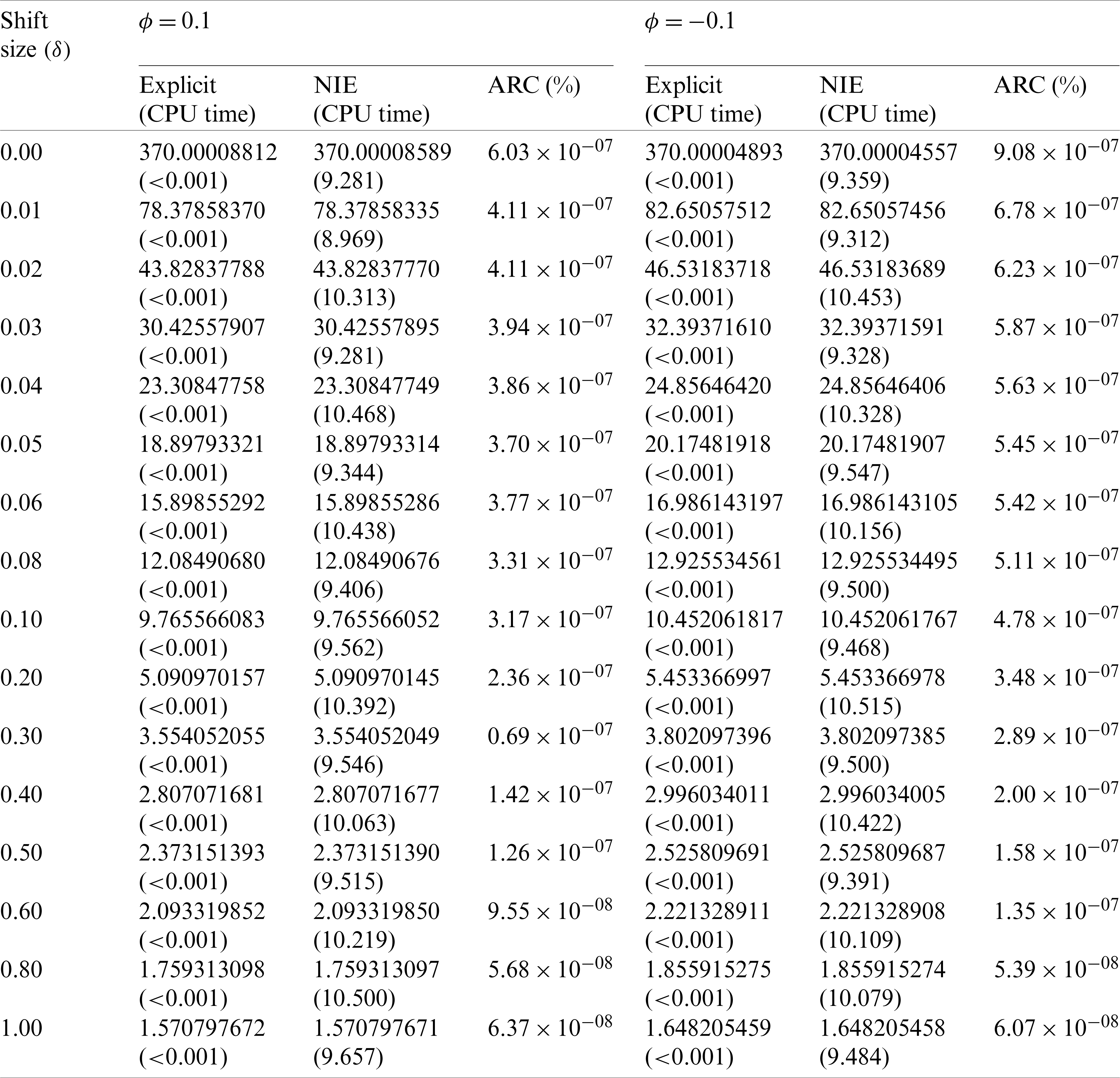
The performance comparison of the explicit formula and the NIE method is explained with the ARL, the ARC and the CPU time (Tab. 1). The first results indicate that the ARL values of the explicit formula are similar to those of the NIE method according to the ARC criterion such that ARC solutions are very low and converge to 0. For the CPU time for calculating the ARL, the explicit formula is faster than the NIE method by around 9 s.

Table 1: Comparison of ARL values on the modified EWMA control chart with the AR(1) model using explicit formulas against the NIE method given λ=0.05, η=2, r = 1, a = 0 at ϕ=0.1 (b = 0.333987011), ϕ=-0.1 (b = 0.408730497) for ARL0=370

The performance of the modified EWMA control chart on varying scales of constant r, different bound control limits [a, b] and various λ are further tested by using the relative mean index (RMI) [34] which can be written as:

where ARLi(c) is the ARL of the control chart for the shift size of row i, ARLi(s) is the smallest ARL of all of the control charts on row i and the RMI value is smaller, then the control chart has more performance for detecting shifts.

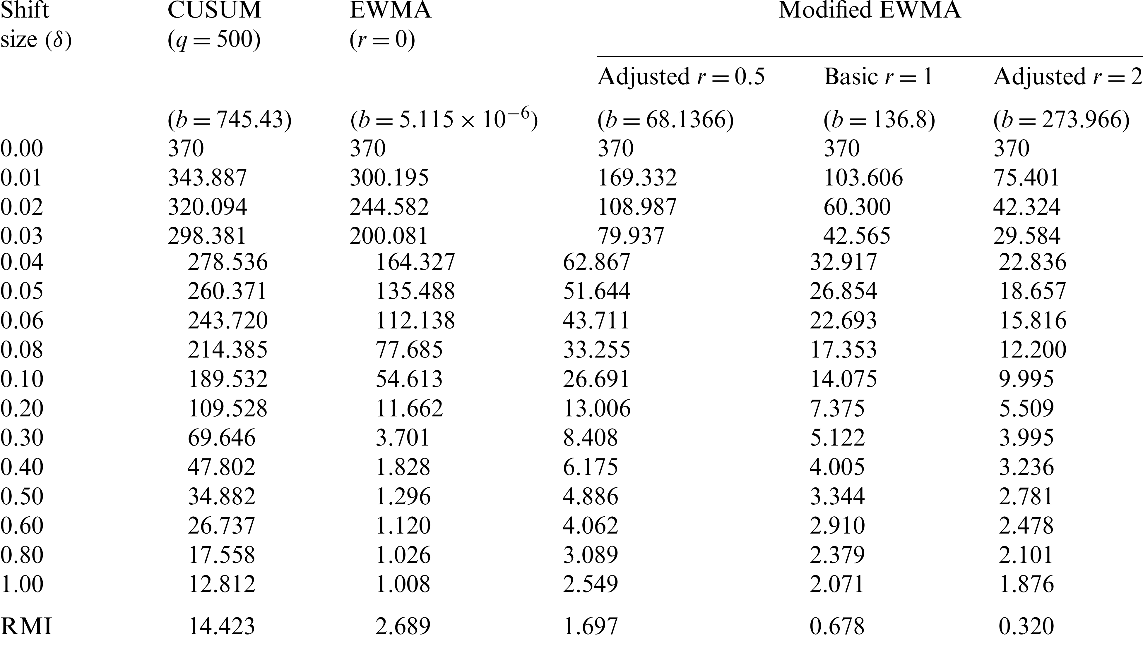
The CUSUM, the classical EWMA (r = 0), the classical modified EWMA (r = 1) and the modified EWMA control charts with adjusted r = 0.5 and r = 2 measured a capability by using the ARL and the RMI at ϕ=0.2, −0.2 for ARL0=370 are compared and reported in Tab. 2 and Fig. 2. When the process mean is shifted, the ARL results of the modified EWMA control charts have abrupt decrease and lower values in small and intermediate shifts. For large shifts, the classical EWMA chart is obtained the least ARL. Therefore, the performance of modified EWMA control charts is better than the classical EWMA scheme for small and intermediate shifts. Moreover, the results show that the CUSUM chart has lower performance than modified EWMA control charts for all levels of shifts. From ARL and RMI comparisons, the modified EWMA control charts with higher r values are more effective.

Table 2: Comparison of the ARL values between the CUSUM, the classical EWMA and modified EWMA control charts given λ=0.05, η=2, a = 0 at ARL0=370

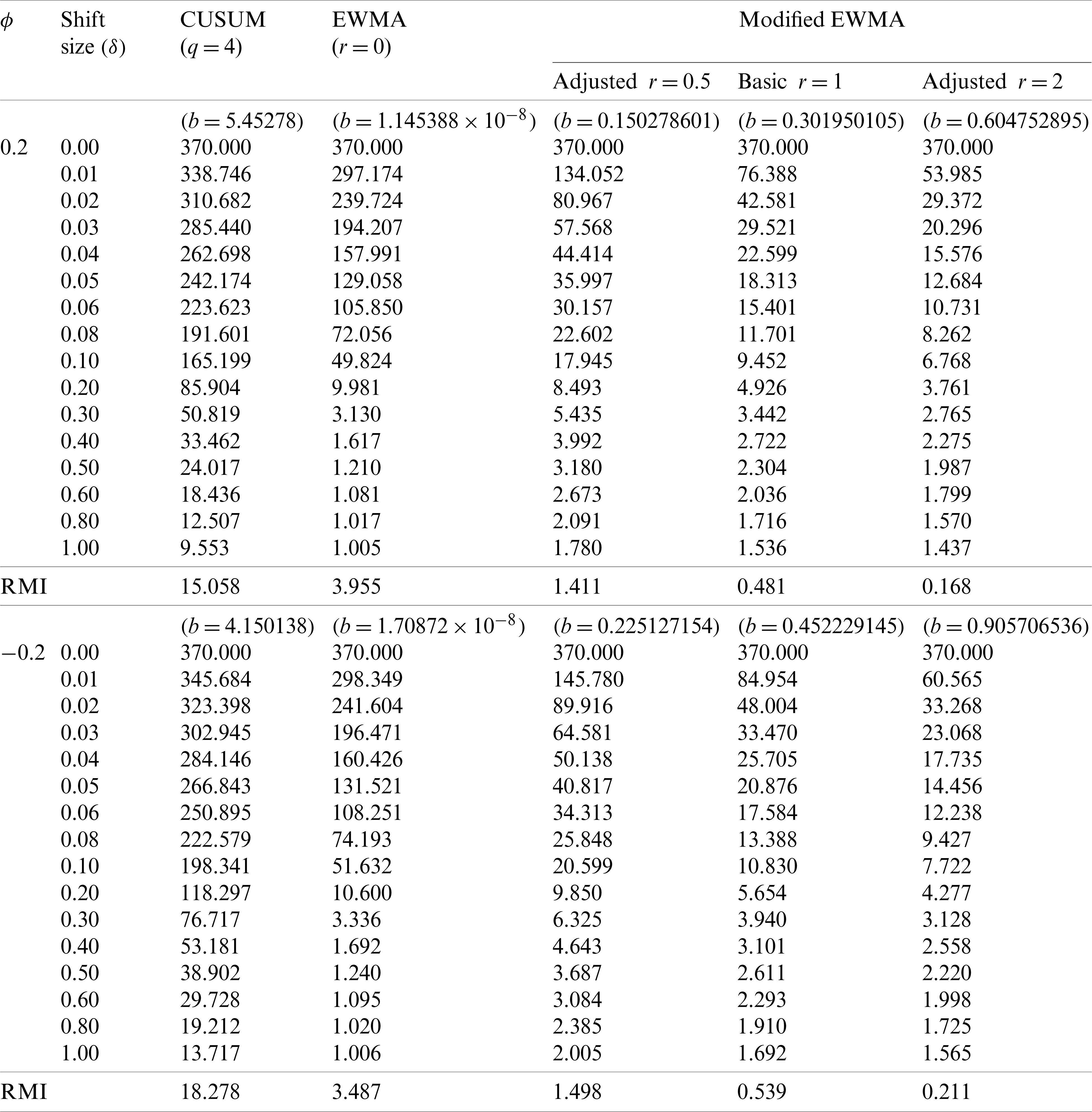
Figure 2: Plot of the CUSUM, the classical EWMA and modified EWMA control charts given (a) ϕ=0.2 and (b) ϕ=-0.2

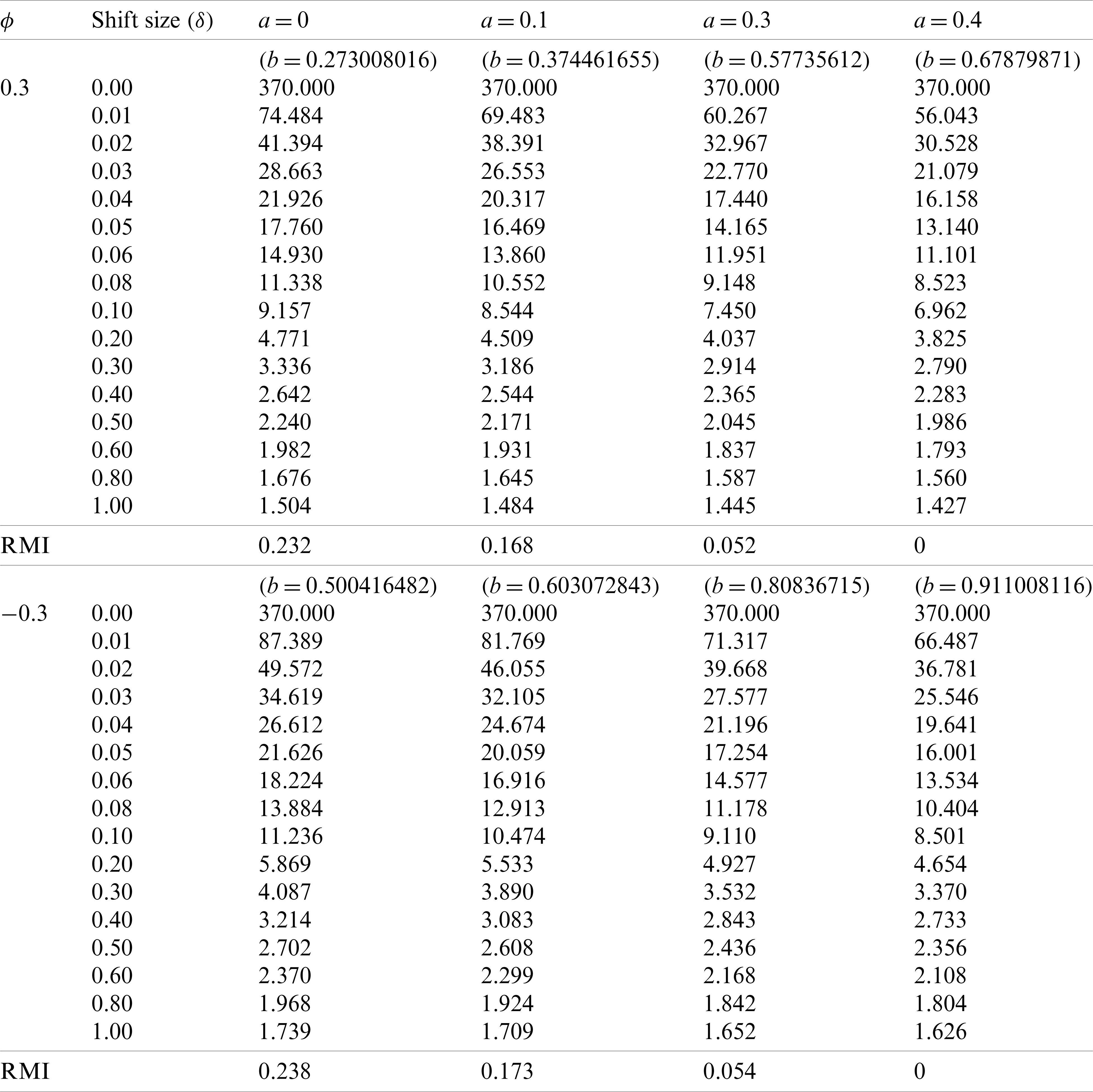
For Tab. 3, the ARL results with ARL0=370 show the performance of the modified EWMA control chart on various bound control limits [a, b] for ϕ=0.3, −0.3 and a = 0, 0.1, 0.3, 0.4. The RMI values of the lower bound a = 0.4 are 0. When the lower bound (a) is higher, then the modified EWMA control chart can detect better shifts when comparing the ARL and the RMI values in one direction.

Table 3: Comparison of the ARL values on the modified EWMA control chart with difference control bounds given λ=0.05, η=2, r = 1 at ARL0=370

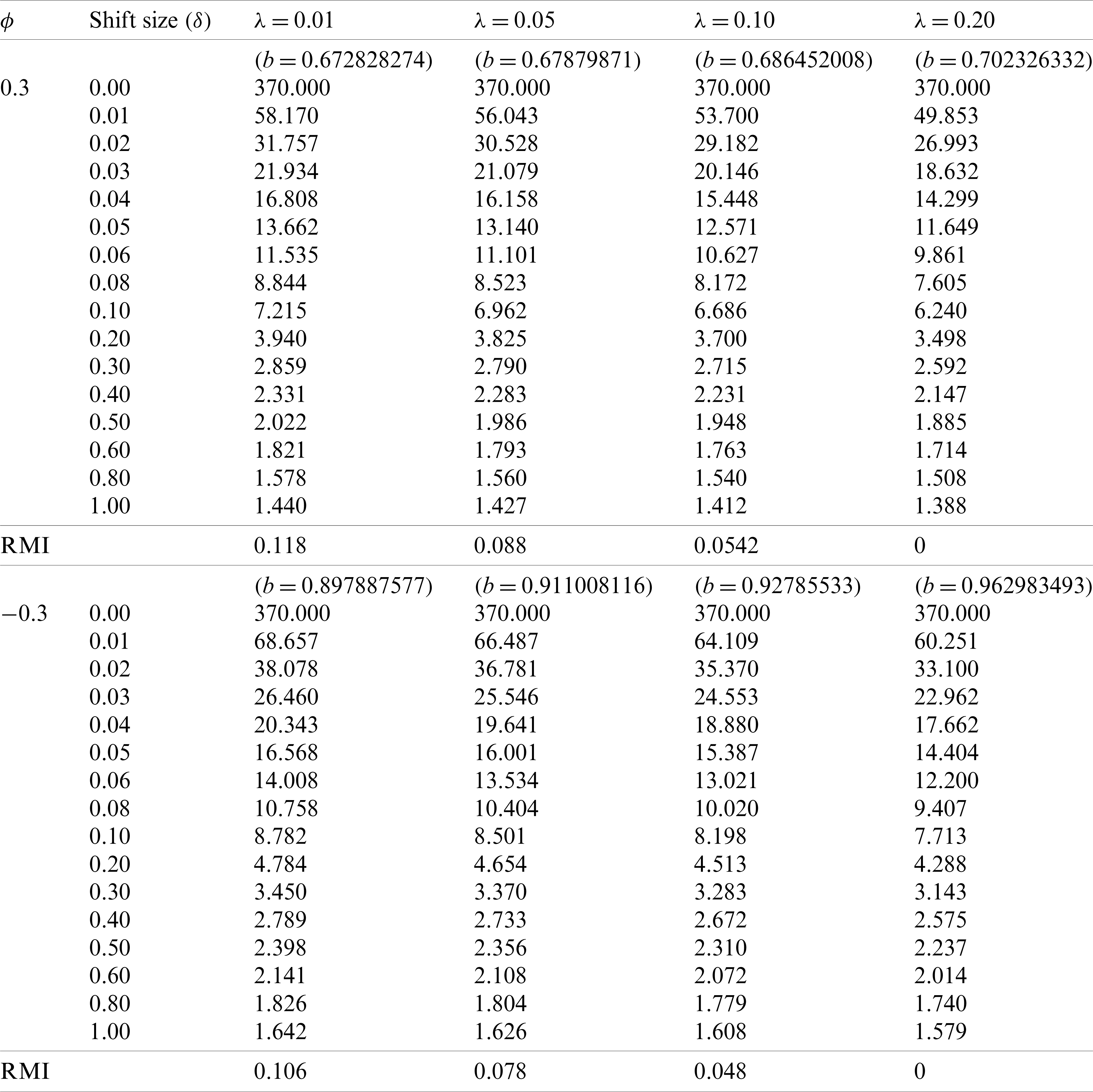
Moreover, the modified EWMA control chart is compared for various λ = 0.01, 0.05, 0.10 and 0.20 at ARL0=370, a = 0.4 and ϕ=0.3, −0.3 (Tab. 4). The RMI values of λ=0.20 are 0. The ARL and the RMI results show that more λ values affect for increasing a detected performance of the modified EWMA control chart.

Table 4: Comparison of the ARL values on the modified EWMA control chart with various λ given η=2, r = 1, a = 0.4 at ARL0=370

As an example, the modified EWMA control chart is applied to COVID-19 data in Thailand and Singapore [35,36] such that the 100 days of newly infected cases are studied when the more summation of 100 cases. These data are checked to a suitable AR(1) process with an exponential white noise at parameters of COVID-19 data in Thailand β0=34.78, η=10.06, ϕ=0.664 and Singapore β0=159.47, η=48.99, ϕ=0.863. Moreover, their error term have be tested an exponential distribution and plotted graphs in Figs. 3 and 4, respectively.

From Tabs. 5 and 6, the results of ARL and the RMI are used to compare the CUSUM, the classical EWMA and modified EWMA control charts with real-world data of COVID-19 data in Thailand and Singapore. The results are in accordance with the simulation data in Tab. 2 and show that the modified EWMA control chart adjusted for high r performs well for small and intermediate level shifts.

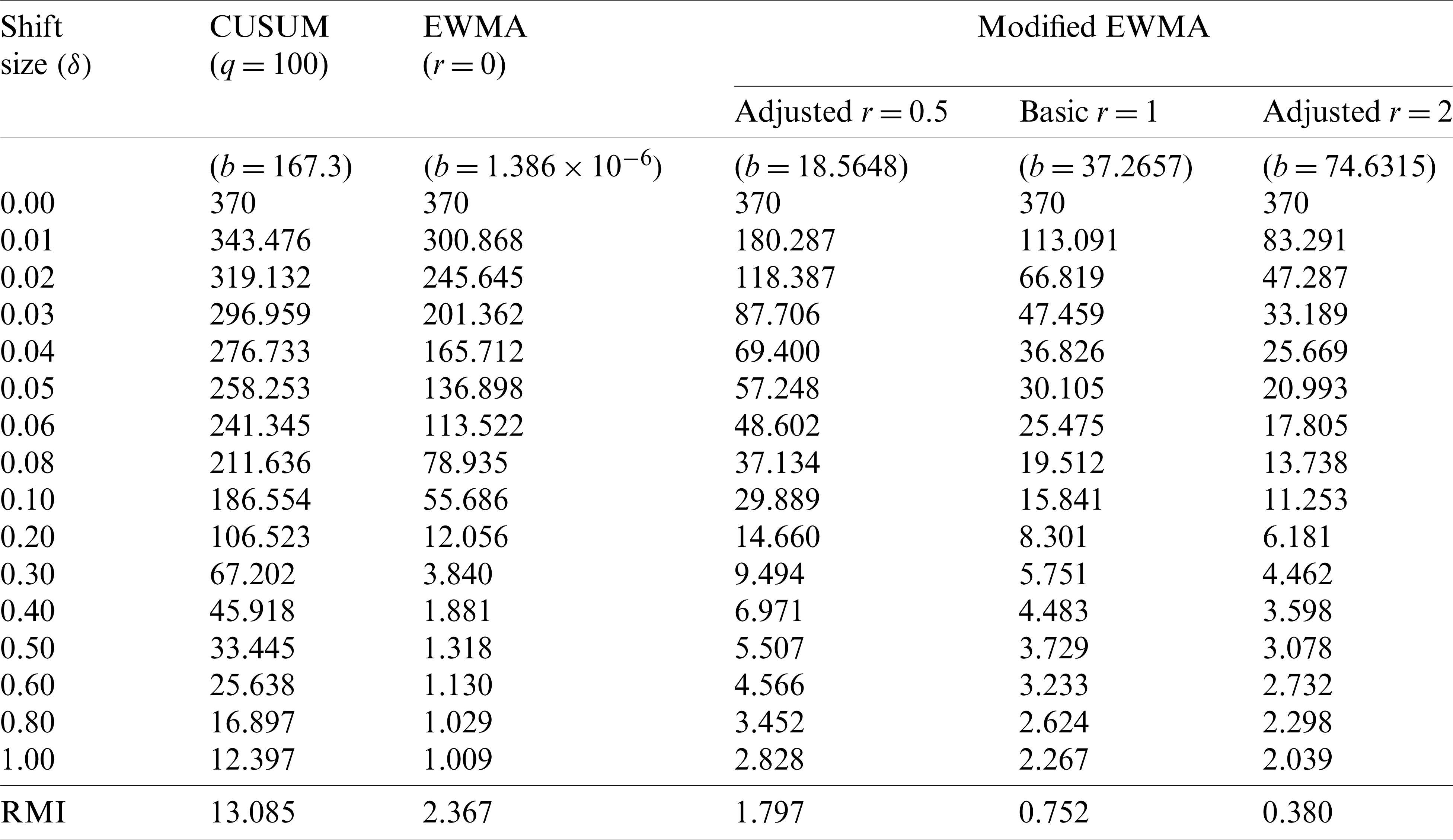
Table 5: Comparison of ARL values between the CUSUM, the classical EWMA and modified EWMA control charts for COVID-19 data in Thailand with β0=34.78, η=10.06, ϕ=0.664, a = 0 at λ=0.05 and ARL0=370

Table 6: Comparison of ARL values between the CUSUM, the classical EWMA and modified EWMA control charts for COVID-19 data in Singapore with β0=159.47, η=48.99, ϕ=0.863, a = 0 at λ=0.05 and ARL0=370

In Fig. 5, the modified EWMA control chart with r = 2 and the classical EWMA control chart are plotted by calculating Zt of COVID-19 data in Thailand and Singapore at the exponential smoothing parameter λ=0.05 with the optimal control width limit of EWMA chart L = 2.615 [37] and the calculated control width limit of the modified EWMA chart Lm = 0.204 at bound control limits of Thailand [10.92, 49.84] and bound control limits of Singapore [519.16, 237]. The results show that Zt values of the modified EWMA control chart with r = 2 exceed the bound since the 4th observation, while Zt values of the classical EWMA control chart are the out-of-control limit at the 9th observation for Thailand. In Singapore, Zt values of the modified EWMA control chart with r = 2 exceed the bound since the first observation, while the classical EWMA control chart signals an alarm in the 10th observation. Therefore, the modified EWMA control chart can detect shifts more quickly than the classical EWMA control chart.

Figure 5: Plot of the classical EWMA and modified EWMA control chart with r = 2 for COVID-19 data in (a) Thailand and (b) Singapore

The performance of a control chart can be evaluated by using the ARL. In this paper, the explicit formula and the numerical integral equation (NIE) method of ARL solutions are established on a two-sided modified EWMA control chart for an AR(1) process with an exponential white noise. The ARL results of both methods are computed and their performances compared via the ARC and the CPU time. The explicit formula shows the actual values of the ARL and is faster calculation than the NIE approach. Moreover, the ARL and RMI results are compared between the CUSUM, the classical and modified EWMA control charts with various r, for which the latter provides better detection for small and intermediate shifts. Next, the performance of the modified EWMA control chart is tested on various bound control limits and is found to be better for higher upper bound values. In addition, this model is applied to the real-world data (COVID-19 data in Thailand and Singapore), with which it obtains similar results as with the simulated data; this result supports the excellent performance of the modified EWMA control chart. In future research, we will establish the optimal bound control limits of the modified EWMA control chart and hope to extend our approach to many new control charts currently under development for different processes.

Funding Statement: The research was supported by King Mongkut’s University of Technology North Bangkok Contract No. KMUTNB-62-KNOW-018.

Conflicts of Interest: The authors declare that they have no conflicts of interest to report regarding the present study.

References

Kovarik, M., Sarga, L., & Klimek, P. (2015). Usage of control charts for time series analysis in financial management. Journal of Business Economics and Management, 16(1), 138-158. [Google Scholar] [CrossRef]
Ozilgen, S. (2011). Statistical quality control charts: New tools for studying the body mass index of populations from the young to the elderly. Journal of Nutrition, Health & Aging, 15(5), 333-334. [Google Scholar] [CrossRef]
Poovarasan, R., Keerthi, S., Yuvashree, K., & Thirumalai, C. (2018). Analysis on diabetes patients using Pearson, cost optimization, control chart. Proceedings of the International Conference on Trends in Electronics and Informatics, 1, 1139-1142. [Google Scholar] [CrossRef]
Montgomery, D. C. (2013). Introduction to statistical quality control. New Jersey: John Wiley & Sons.
Roberts, W. S. (1959). Control chart tests based on geometric moving averages. Technometrics, 1(3), 239-250. [Google Scholar] [CrossRef]
Page, E. S. (1954). Continuous inspection schemes. Biometrika, 41(1–2), 100-115. [Google Scholar] [CrossRef]
Patel, A. K., & Divecha, J. (2011). Modified exponentially weighted moving average (EWMA) control chart for an analytical process data. Journal of Chemical Engineering and Materials Science, 2, 12-20. [Google Scholar] [CrossRef]
Khan, N., Aslam, M., & Jun, C. H. (2017). Design of a control chart using a modified EWMA statistic. Quality and Reliability Engineering International, 33(5), 1095-1104. [Google Scholar] [CrossRef]
Khusna, H., Mashuri, M., Suhartono, S., Prastyo, D. D., & Ahsan, M. (2018). Multioutput least square SVR-based multivariate EWMA control chart: The performance evaluation and application. Cogent Engineering, 5(1), 1-14. [Google Scholar] [CrossRef]
Flury, M. I., & Quaglino, M. B. (2018). Multivariate EWMA control chart with highly asymmetric gamma distributions. Quality Technology & Quantitative Management, 15(2), 230-252. [Google Scholar] [CrossRef]
Chananet, C., Areepong, Y., & Sukparungsee, S. (2015). A markov chain approach for average run length of EWMA and CUSUM control chart based on ZINB Model. International Journal of Applied Mathematics and Statistics, 53(1), 126-137. [Google Scholar]
Sukparungsee, S. (2012). Combining martingale and integral equation approaches for finding optimal parameters of EWMA. Applied Mathematical Sciences, 6, 4471-4482. [Google Scholar]
Suriyakat, W., Areepong, Y., Sukparungsee, S., & Mititelu, G. (2012). On EWMA procedure for AR(1) observations with exponential white noise. International Journal of Pure and Applied Mathematics, 77, 73-83. [Google Scholar]
Busaba, J., Sukparungsee, S., & Areepong, Y. (2012). Numerical approximations of average run length for AR(1) on exponential CUSUM. Proceedings of the International MultiConference of Engineers and Computer Scientists, 2, 1268-1273. [Google Scholar]
Petcharat, K., Sukparungsee, S., & Areepong, Y. (2015). Exact solution of the average run length for the cumulative sum chart for a moving average process of order q. ScienceAsia, 41(2), 141-147. [Google Scholar] [CrossRef]
Peerajit, W., Areepong, Y., & Sukparungsee, S. (2018). Numerical integral equation method for ARL of CUSUM chart for long-memory process with non-seasonal and seasonal ARFIMA models. Thailand Statistician, 16(1), 26-37. [Google Scholar]
Sukparungsee, S., & Areepong, Y. (2017). An explicit analytical solution of the average run length of an exponentially weighted moving average control chart using an autoregressive model. Chiang Mai Journal of Science, 44(3), 1172-1179. [Google Scholar]
Sunthornwat, R., Areepong, Y., & Sukparungsee, S. (2017). Average run length of the long-memory autoregressive fractionally integrated moving average process of the exponential weighted moving average control chart. Cogent Mathematics, 4(1), 1-11. [Google Scholar] [CrossRef]
Sunthornwat, R., Areepong, Y., & Sukparungsee, S. (2018). Average run length with a practical investigation of estimating parameters of the EWMA control chart on the long memory AFRIMA process. Thailand Statistician, 16(2), 190-202. [Google Scholar]
Peerajit, W., Areepong, Y., & Sukparungsee, S. (2019). Explicit analytical solutions for ARL of CUSUM chart for a long-memory SARFIMA model. Communications in Statistics–Simulation and Computation, 48(4), 1176-1190. [Google Scholar] [CrossRef]
Vanhatalo, E., & Kulahci, M. (2014). The effect of autocorrelation on the Hotelling control chart. Quality and Reliability Engineering International, 31(8), 1779-1796. [Google Scholar] [CrossRef]
He, Z., Wang, Z., Tsung, F., & Shang, Y. (2016). A control scheme for autocorrelated bivariate binomial data. Computers and Industrial Engineering, 98, 350-359. [Google Scholar] [CrossRef]
Kim, H., & Lee, S. (2017). On first-order integer-valued autoregressive process with Katz family innovations. Journal of Statistical Computation and Simulation, 87(3), 546-562. [Google Scholar] [CrossRef]
Yadav, V., & Nath, S. (2017). Forecasting of using autoregressive models and exponential smoothing technique. Asian Journal of Water, Environment and Pollution, 14(4), 109-113. [Google Scholar] [CrossRef]
Shapoval, A., Mouel, J. L. L., Shnirman, M., & Courtillot, V. (2015). Stochastic description of the high-frequency content of daily sunspots and evidence for regime changes. Astrophysical Journal, 799(1), 1-8. [Google Scholar] [CrossRef]
Hirsch, S., & Hartmann, M. (2014). Persistence of firm-level profitability in the European dairy processing industry. Agricultural Economics, 45(1), 53-63. [Google Scholar] [CrossRef]
Andel, J. (1988). On AR(1) processes with exponential white noise. Communications in Statistics–Theory and Methods, 17(5), 1481-1495. [Google Scholar] [CrossRef]
Fellag, H., & Ibazizen, M. (2001). Estimation of the first-order autoregressive model with contaminated exponential white noise. Journal of Mathematical Sciences, 106(1), 2652-2656. [Google Scholar] [CrossRef]
Pereira, I., & Amaral-Turkman, M. A. (2004). Bayesian prediction in threshold autoregressive models with exponential white noise. Test, 13(1), 45-64. [Google Scholar] [CrossRef]
Champ, C. W., & Rigdon, S. E. (1991). A comparison of the Markov Chain and the integral equation approaches for evaluating the run length distribution of quality control charts. Communication in Statistics–Simulation, 20(1), 191-203. [Google Scholar] [CrossRef]
Davison, K. R., Donsig, A. P. (2010). Real analysis with real applications. New York: Springer-Verlag.
Phanthuna, P., Areepong, Y., & Sukparungsee, S. (2018). Numerical integral equation methods of average run length on modified EWMA control chart for exponential AR(1) process. Proceedings of the International MultiConference of Engineers and Computer Scientists, 2, 845-847. [Google Scholar]
Nguyen, Q. T., Tran, K. P., Castagliola, P., Celano, G., & Lardjane, S. (2019). One-sided synthetic control charts for monitoring the multivariate coefficient of variation. Journal of Statistical Computation and Simulation, 89(10), 1841-1862. [Google Scholar] [CrossRef]
Tang, A., Castagliola, P., Sun, J., & Hu, X. (2018). Optimal design of the adaptive EWMA chart for the mean based on median run length and expected median run length. Quality Technology and Quantitative Management, 16(4), 439-458. [Google Scholar] [CrossRef]
WHO (2020). Thailand situation reports: Coronavirus disease (COVID-19) dashboard. https://covid19.who.int/region/wpro/country/sg.
WHO (2020). Singapore situation reports: Coronavirus disease (COVID-19) dashboard. https://covid19.who.int/region/searo/country/th.
Lucas, J. M., & Saccucci, M. S. (1990). Exponentially weighted moving average control schemes: Properties and enhancements. Technometrics, 32(1), 1-12. [Google Scholar] [CrossRef]