| Computer Modeling in Engineering & Sciences |
DOI: 10.32604/cmes.2021.014635
ARTICLE
Stereo Matching Method Based on Space-Aware Network Model
1College of Information & Computer Engineering, Northeast Forestry University, Harbin, 150040, China
2College of Computer & Information Technology, Mudanjiang Normal University, Mudanjiang, 157011, China
*Corresponding Author: Jilong Bian. Email: bianjilong@nefu.edu.cn
Received: 14 October 2020; Accepted: 11 January 2021
Abstract: The stereo matching method based on a space-aware network is proposed, which divides the network into three sections: Basic layer, scale layer, and decision layer. This division is beneficial to integrate residue network and dense network into the space-aware network model. The vertical splitting method for computing matching cost by using the space-aware network is proposed for solving the limitation of GPU RAM. Moreover, a hybrid loss is brought forward to boost the performance of the proposed deep network. In the proposed stereo matching method, the space-aware network is used to calculate the matching cost and then cross-based cost aggregation and semi-global matching are employed to compute a disparity map. Finally, a disparity-post processing method is utilized such as subpixel interpolation, median filter, and bilateral filter. The experimental results show this method has a good performance on running time and accuracy, with a percentage of erroneous pixels of 1.23% on KITTI 2012 and 1.94% on KITTI 2015.
Keywords: Deep learning; stereo matching; space-aware network; hybrid loss
Stereo matching is an important research topic in the field of computer vision. It is widely used in three-dimensional reconstruction [1], autonomous navigation [2,3], and augmented reality [4]. In the pipeline of stereo matching, an input of stereo matching consists of two epipolar rectified images taken from different points of view, one of which serves as a reference image and the other as a matching image. For each pixel
Stereo matching process is divided into four steps: Cost calculation, cost aggregation, disparity calculation, and disparity refinement [5]. Cost calculation is the first step in stereo matching process, and its quality largely affects the accuracy of stereo matching. For the past few years, deep learning has made great progress and is widely applied in intelligent traffic [6–9], network security [10–14], privacy-protecting [15–18], and natural language processing [19–21]. Recently, deep learning has also been applied to stereo matching to calculate matching cost because of its powerful feature representation ability. It can improve the robustness of matching cost to radiation difference and geometric distortion and enhance matching accuracy. Lecun et al. [22,23] first employs Siamese network structure [24] to calculate matching cost, the matching cost is aggregated by the cross-based cost aggregation method, a disparity map is produced by the semi-global matching method [25], and finally, a disparity map is refined using some disparity post-processing methods. Subsequently, Zagoruyko et al. [26] extends the Siamese network structure and proposes three network structures, which are applied to stereo matching to calculate matching cost. Chen et al. [27] put forward a deep embedding model, which was like the central-surrounding two-stream network [26]. Luo et al. [28] propose an efficient deep learning model, which takes image patches of different sizes as input of left and right branch networks. The right image patch is larger than the left image patch in size and contains all disparities. In stereo matching, deep learning is used to calculate matching cost, which has achieved good matching results. This kind of method associates the depth of a network model with the size of training patches and the network depth depends on the size of a training image patch. As a result, it is impossible to increase the network depth to achieve high matching accuracy without changing the size of training image patches, which makes this method unable to effectively use excellent deep network structures such as residual network [29] and dense network [30].
To increase the depth of the network and improve matching accuracy, we propose a stereo matching method based on the space-aware network. Firstly, matching cost is calculated by using a deep network, then the matching cost is aggregated by cross-based cost aggregation method, and a disparity map is computed by the semi-global method. Finally, the disparity map is further refined by some disparity post-processing methods. The main contributions of this paper are as follows: Firstly, we propose a space-aware network model, which can have the ability to integrate many popular network models. Secondly, a hybrid loss function is designed to enhance the network performance. Finally, a vertical splitting method is proposed to calculate feature maps for a whole image to reduce the consumption of GPU memory.
Deep learning is applied to calculation of matching cost and can produce good matching results [23]. The deep network is called Siamese network, which consists of two parts: Feature layer and decision layer, and its network structure is shown in Fig. 1. The feature layer is composed of two branches with the same structure and weight, which receive an image patch, respectively. The two image patches are fed into convolution layers, ReLU layers, and max-pooling layers. When they pass through a convolution layer, their size will be decreased. Finally, each branch obtains a one-dimensional feature vector, and these two feature vectors are concatenated and fed into a decision layer. The decision layer consists of a linear fully connected layer followed by a ReLU layer and outputs a scalar value, which is a probability value and denotes whether left and right image patches are similar. Fig. 1 shows a deep network including 4 convolution layers with a convolution kernel of size
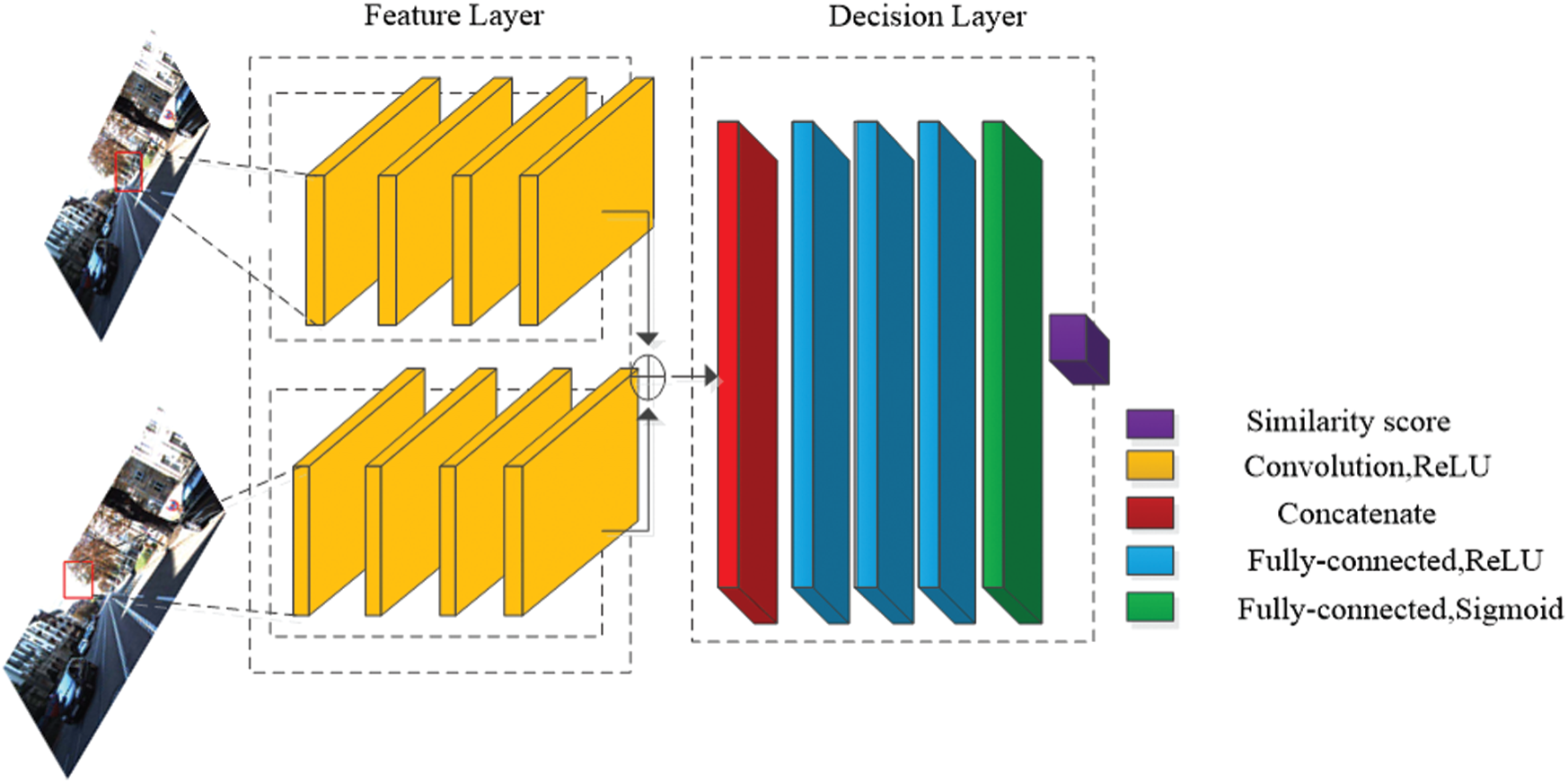
Figure 1: Deep network for stereo matching
He et al. [29] proposed a residual network model, which has been applied to image classification and achieved very good results. Up to now, it is still a popular network model and there are many variants. The basic idea of this model is to add an Identity Shortcut Connection to the network model, which skips several convolution layers at one time. A residual block structure is shown in Fig. 2. A residual block can be expressed as
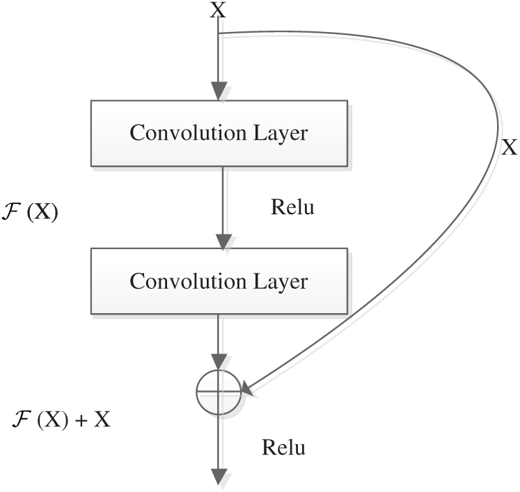
Figure 2: Residual block
The idea of residual connection is extended to propose a dense connection network [30]. As shown in Fig. 3, each convolution layer in a dense block has an Identity Shortcut Connection connecting to the convolution layers coming before it. The input of each convolution layer is made of the concatenation of feature maps of all convolution layers coming behind it along feature dimension. A layer in a dense block can be denoted as
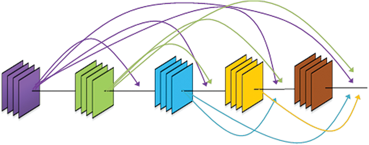
Figure 3: Dense block
For each pixel p in a reference image, stereo matching first calculates matching cost
To solve this problem and use a more advanced network model to calculate the stereo matching cost, we propose a space-aware network model. The main characteristic of this model is that the feature layer is divided into two parts: Basic layer and scaling layer. The main purpose of the basic layer is to extract features, which can use advanced network models such as residual network and dense network. Fig. 4 shows the overall structure of the space-aware network model. The input of the basic layer is a pair of the image patches
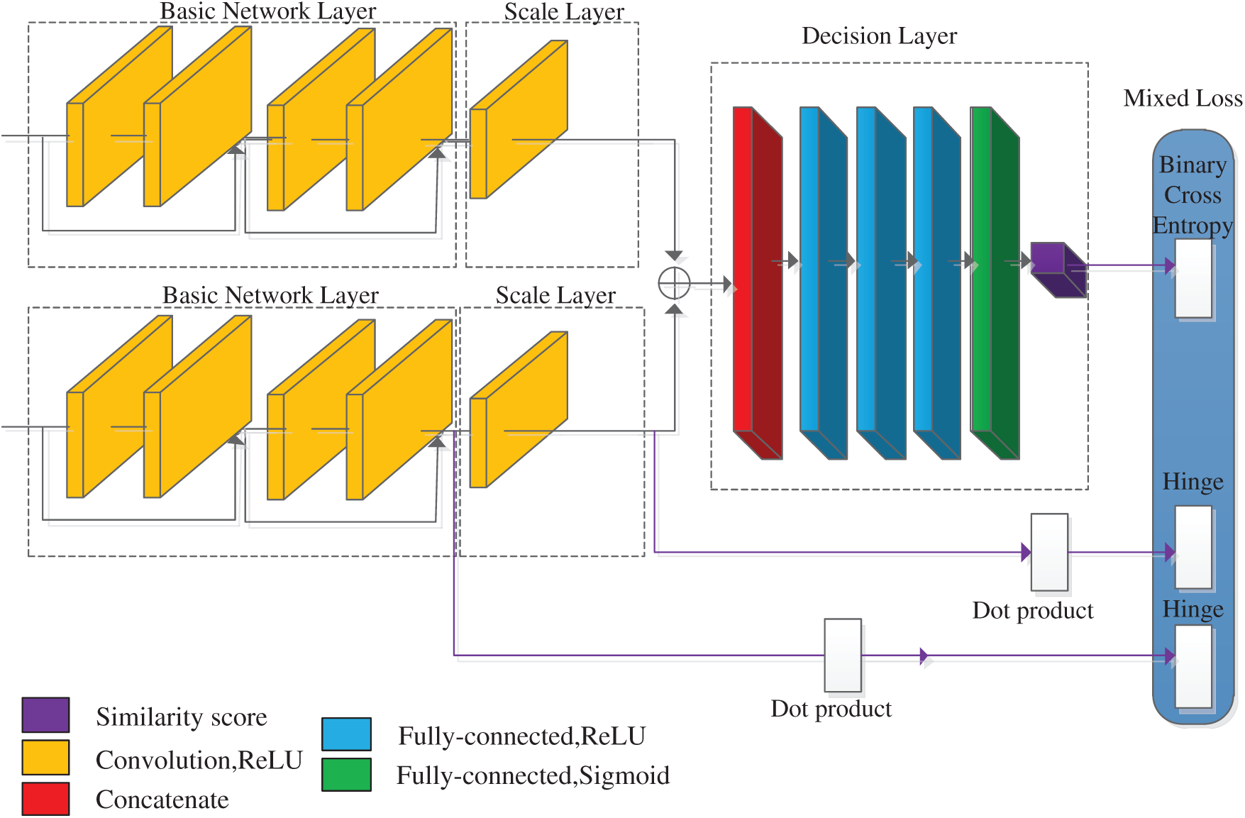
Figure 4: Space-aware network
Because the proposed network model consists of three parts: Basic layer, scaling layer and decision layer, we combine the outputs of these three parts to define a hybrid loss function. The outputs of two branches of the basic layer are flattened to a one-dimensional vector, and then the cosine similarity is calculated by using an inner product layer:
where uL and uR denote the output of the left and right branches of the basic layer. The output of the left and right branches in the scaling layer is a one-dimensional vector, so we do not need to flatten the scaling layer output and can directly utilize the cosine similarity. Because ReLU is used as an activation function, the output of the network is greater than 0, and the output range of the inner product layer is [0, 1]. For these two outputs, Hinge loss is used:
where
where v+ and v − are outputs of the decision layer for positive and negative samples. Finally, the total loss is:
where
During training, the proposed deep network produces three outputs: One output of the decision layer and two outputs of the inner product layer, but only the output of the decision layer is used as matching cost to compute disparities:
where
Therefore, we propose a vertical splitting method to reduce the consumption of GPU memory. The main idea of this method is to divide left and right images into several patches vertically:
where py denotes vertical coordinate of p and K denotes patch height. Then, an initial cost volume is produced for each pair of vertical patches using the space-aware network:
where
The output of the space-aware network is an initial 3D cost volume. Cost aggregation, disparity calculation, and disparity postprocessing are used to obtain a more accurate disparity map. Firstly, cross-based cost aggregation is employed, and secondly, semi-global matching is adopted. Finally, a series of disparity post-processing methods are utilized, such as left-right consistency check, sub-pixel enhancement, median filtering, and bilateral filtering.
5.1 Cross-Based Cost Aggregation
The cross-based cost aggregation method [31] firstly constructs a cross arm for each pixel, then uses cross arms to define a supporting area for each pixel. A left-arm of the pixel p can be defined as:
where
Then, cost aggregation is carried out on the supporting area
where
Disparity calculation is usually classified into a local optimization method and a global optimization method. Global optimization methods generally obtain a high accuracy map, including dynamic programming, belief propagation, and graph-cut optimization. A global optimization method transforms the stereo matching problem into an energy function minimization problem:
where D denotes a disparity map,
where r denotes direction and
Then, disparities are calculated by the “winner-takes-all” method:
To improve the accuracy of stereo matching, we use disparity post-processing methods such as left-right consistency check, sub-pixel enhancement, median filtering, and bilateral filtering. There are inevitably some erroneous disparities in a disparity map, which may be caused by non-textured areas and occlusion. These erroneous disparities can be detected by left-right consistency check of left and right disparity maps, and each pixel can be marked by the following rules:
where
Sub-pixel refinement can further improve matching accuracy. We use a sub-pixel refinement method based on quadratic curve fitting in the cost domain, which uses optimal matching cost and its left and right immediate matching costs to fit a quadratic curve to obtain a sub-pixel-level disparity:
where
The final step of stereo matching uses a
where
We use LUA and Torch7 to implement the proposed stereo matching method based on a deep space-aware network and the network is trained on GeForce GTX1080Ti GPU. The experimental parameters are set as
The choice of training strategy is very important for deep learning, and a good training strategy can accelerate convergence and improve accuracy. In our experiment, the SGD optimizer algorithm is adopted, and its momentum is set to 0.9. The learning rate adjustment method is OneCycleLR with a cosine annealing strategy and the initial learning rate is set to 0.003. Its learning rate curve is shown in Fig. 5. The space-aware network is trained for 14 epochs.
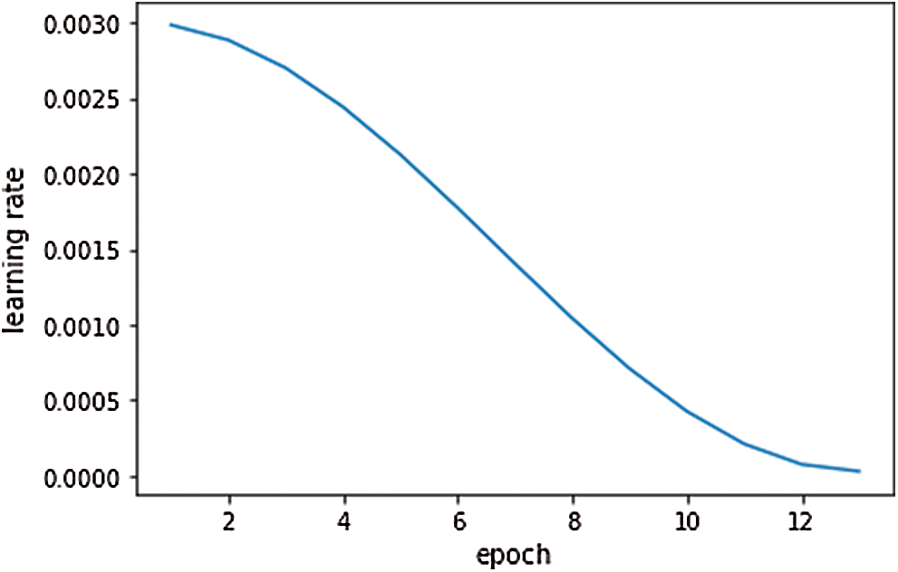
Figure 5: Learning rate curve
6.2 Classification Accuracy Analysis
The computation of matching cost with deep learning is a binary classification problem. The higher the classification accuracy is, the more accurate the matching cost is, and the higher the matching accuracy is. In this experiment, 80% of training data is used as training data and 20% as validation data to analyze the classification accuracy of the proposed network model. The comparison of classification accuracy is shown in Fig. 6a, which indicates that the validation accuracy increases steadily with the increase of training epochs, and our classification accuracy is 98.40%. With the increase of epochs, the classification accuracy of [22] shows a slight fluctuation and its classification accuracy is 94.25%. We also compare training loss and validation loss. The comparison of training loss is shown in Fig. 6b, which indicates that our proposed method obtains lower training loss and better convergence effect. Fig. 6c shows validation loss. With the increase of epochs, the validation loss of our proposed method gradually decreases, and our validation loss is lower than [22], which shows that our network model is better than [22].
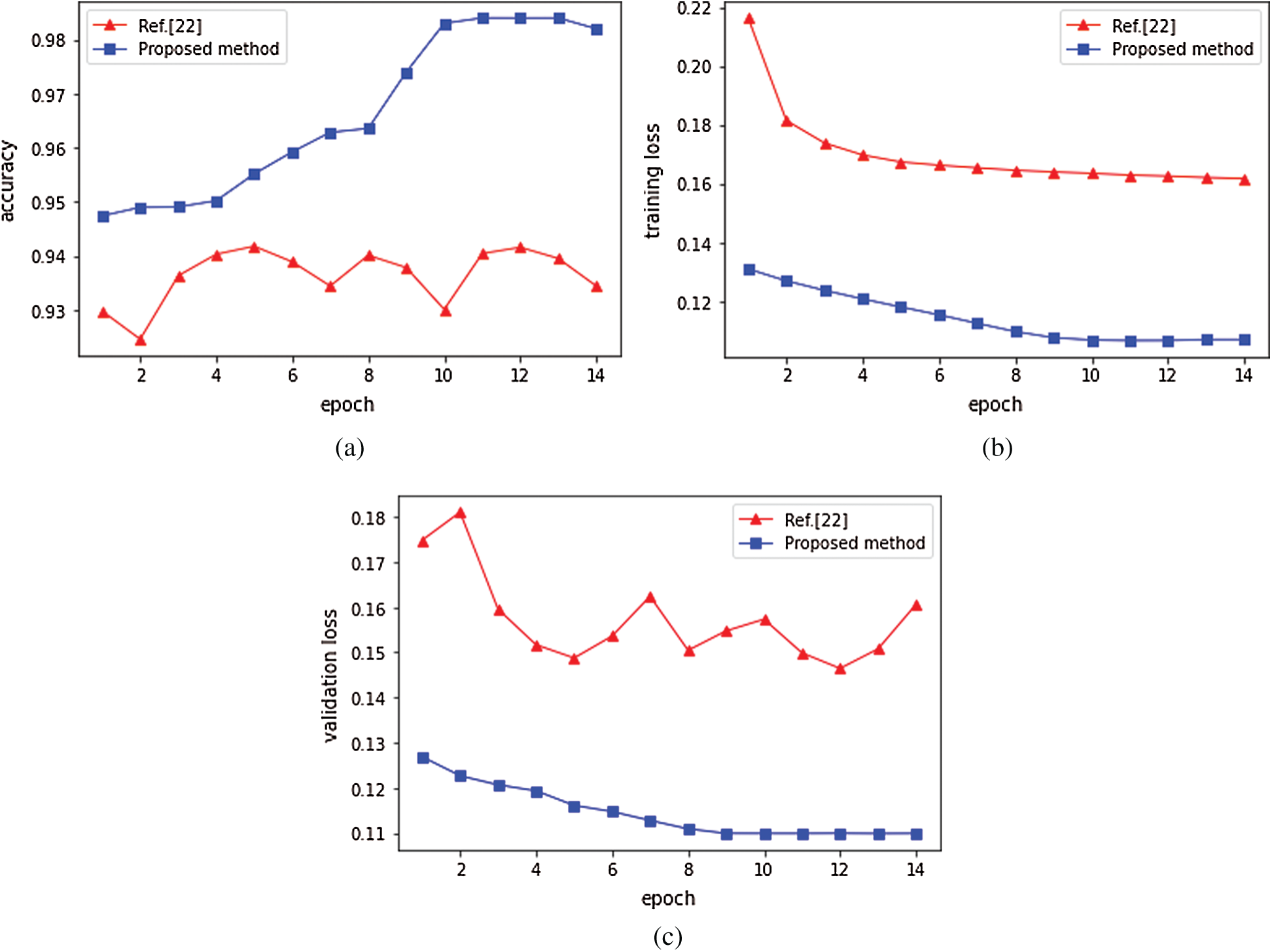
Figure 6: Classification accuracy and loss for the proposed method and Ref. [22]. (a) Classification accuracy (b) Training loss (c) Validation loss
6.3 Matching Accuracy Analysis
In this paper, we implement two space-aware network models. In the first network called SADenseNet, DenseNet with 20 DenseNet blocks is selected as the feature layer, the scale layer consists of a convolutional layer with the filter kernel of size
Table 1: Comparison result for 2012 dataset

Table 2: Comparison result for 2015 dataset
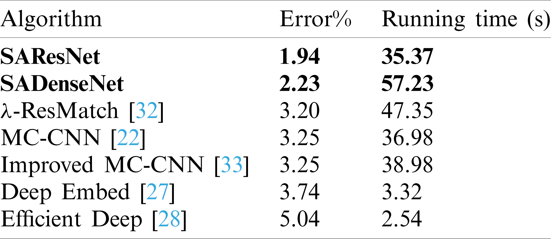
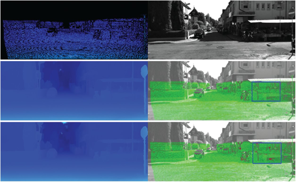
Figure 7: Comparison for disparities map of two proposed deep network
6.4 Comparision of Experimental Results
In this section, we first use the KITTI2012 dataset to test the performance of our proposed stereo matching method based on a space-aware network model and compare it with other methods. We randomly select 40 stereo pairs and compute the average error percentage of 3 pixels. The comparison results are shown in Tab. 1. Our proposed method gives a good performance, whose average error percentage is 1.23%. Fig. 8 shows the calculated disparity maps for four methods with low error percentage. Fig. 8a shows the left and right images and the ground truth, and Fig. 8b shows the calculated disparity and the error map for SAResNet, with an error percentage of 0.65%; Fig. 8c for SADenseNet, with an error percentage of 1.2%; Fig. 8d for [32], with an error percentage of 4.97%; Fig. 8e for [22], with an error percentage of 5.90%. From these error maps, it can be observed that our method can obviously reduce the erroneous pixels in the blue rectangle.
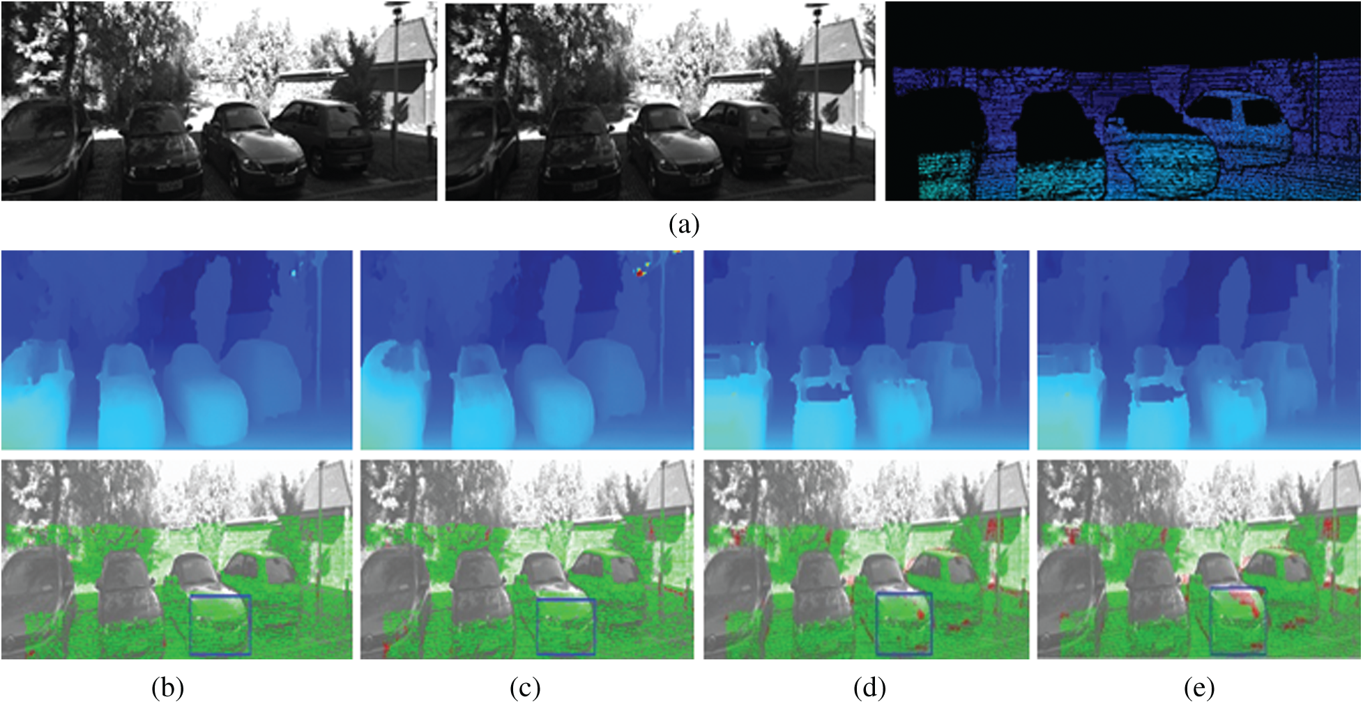
Figure 8: Results of disparity estimation for KITTI 2012. (a) The left and right images and the groud truth (b) SAResNet (c) SADenseNet (d) [32] (e) [22]
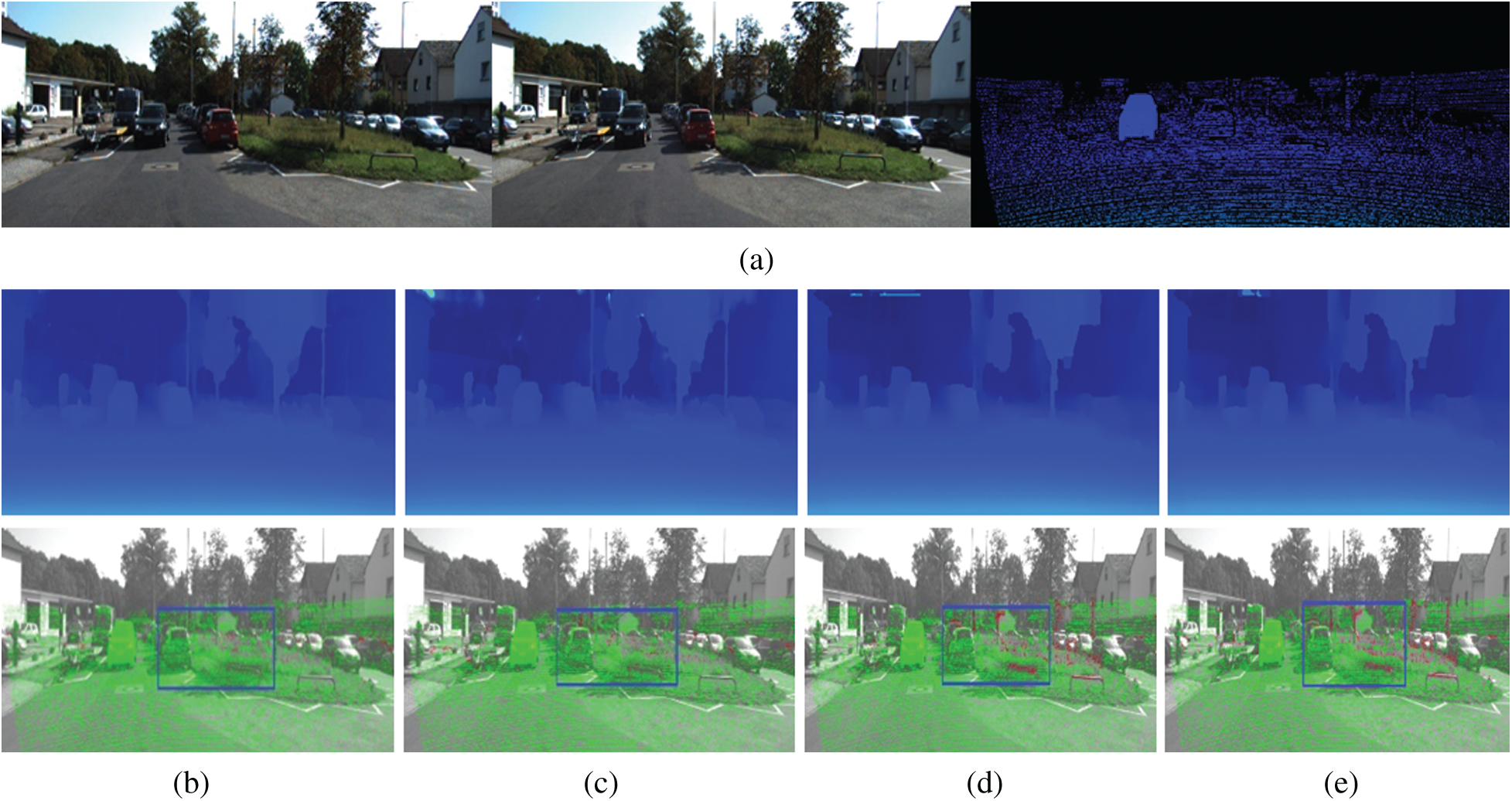
Figure 9: Results of disparity estimation for KITTI 2015. (a) The left and right images and the groud truth (b) SAResNet (c) SADenseNet (d) [32] (e) [22]
In this section, we use the KITTI2015 dataset to test the performance of our space-aware network and compare it with other methods by using the same metric as the KITTI2012 dataset. The comparison results are shown in Tab. 2. Fig. 9 shows the calculated disparity maps for four methods with low error percentage. Fig. 9a shows the left and right images and the ground truth, and Fig. 9b shows the calculated disparity map and the error map for SAResNet with the 3-pixel error percentage of 0.64%; Fig. 9c for SADenseNet with the 3-pixel error percentage of 1.30%; Fig. 9d for [32] with the 3-pixel error percentage of 2.80%; Fig. 9e for [22] with the 3-pixel error percentage of 2.90%. These experimental results show that our proposed method can give a more accurate disparity. The blue rectangles in these error maps show that the erroneous pixels marked by red are less than other methods.
In this paper, a stereo matching method based on the space-aware network is proposed, which can combine the advanced network model with our network model, and then solve the GPU memory limitation problem through a vertical splitting method, and further improve the network performance by using hybrid loss. Our proposed method is trained on KITTI 2012 and KITTI 2015 datasets and compared with other methods. The experimental results show that the proposed method gives a better performance, with an error rate of 1.23% on KITTI 2012 and 1.94% on KITTI 2015.
Funding Statement: This work was supported in part by the Heilongjiang Provincial Natural Science Foundation of China under Grant F2018002, the Research Funds for the Central Universities under Grants 2572016BB11 and 2572016BB12, and the Foundation of Heilongjiang Education Department under Grant 1354MSYYB003.
Conflicts of Interest: The authors declare that they have no conflicts of interest to report regarding the present study.
1. Wang, S., Wu, T. H., Yang, L. F. (2019). Three-dimensional reconstruction of wear particle surface based on photometric stereo. Measurement, 133, 350–360. DOI 10.1016/j.measurement.2018.10.032. [Google Scholar] [CrossRef]
2. Sasiadek, J. Z., Walker, M. J., Yang, L. F. (2019). Achievable stereo vision depth accuracy with changing camera baseline. Proceedings of 24th International Conference on Methods and Models in Automation and Robotics, pp. 152–157, Miedzyzdroje, Poland. [Google Scholar]
3. Ioannidis, V. S. K., Sirakoulis, G. C., Kosmatopoulos, E. B. (2019). Real-time active SLAM and obstacle avoidance for an autonomous robot based on stereo vision. Cybernetics and Systems, 50(3), 239–260. DOI 10.1080/01969722.2018.1541599. [Google Scholar] [CrossRef]
4. Kalia, M., Navab, N., Salcudean, T. (2019). A real-time interactive augmented reality depth estimation technique for surgical robotics. Proceedings of International Conference on Robotics and Automation, pp. 8291–8297, Montreal, QC, Canada. [Google Scholar]
5. Scharstein, D., Szeliski, R., Zabih, R. (2002). A taxonomy and evaluation of dense two-frame stereo correspondence algorithms. International Journal of Computer Vision, 47(1), 7–42. DOI 10.1023/A:1014573219977. [Google Scholar] [CrossRef]
6. Tian, Z., Gao, X., Su, S., Qiu, J. (2020). Vcash: A novel reputation framework for identifying denial of traffic service in internet of connected vehicles. IEEE Internet of Things Journal, 7(5), 3901–3909. DOI 10.1109/JIOT.2019.2951620. [Google Scholar] [CrossRef]
7. Qiu, J., Du, L., Zhang, D., Su, S., Tian, Z. (2020). Nei-TTE: Intelligent traffic time estimation based on fine-grained time derivation of road segments for smart city. IEEE Transactions on Industrial Informatics, 16(4), 2659–2666. DOI 10.1109/TII.2019.2943906. [Google Scholar] [CrossRef]
8. Shafiq, M., Tian, Z., Bashir, A. K., Du, X., Guizani, M. (2020). CorrAUC: A malicious Bot-IoT traffic detection method in IoT network using machine learning techniques. IEEE Internet of Things Journal, 7(5), 1–12. DOI 10.1109/JIOT.2020.3002255. [Google Scholar] [CrossRef]
9. Tian, Z., Gao, X., Su, S., Qiu, J., Du, X. et al. (2019). Evaluating reputation management schemes of Internet of vehicles based on evolutionary game theory. IEEE Transactions on Vehicular Technology, 68(6), 5971–5980. DOI 10.1109/TVT.2019.2910217. [Google Scholar] [CrossRef]
10. Tian, Z., Shi, W., Wang, Y., Zhu, C., Du, X. et al. (2019). Real time lateral movement detection based on evidence reasoning network for edge computing environment. Computer IEEE Transactions on Industrial Informatics, 15(7), 4285–4294. DOI 10.1109/TII.2019.2907754. [Google Scholar] [CrossRef]
11. Tian, Z., Li, M., Qiu, M., Sun, Y., Su, S. (2019). Block-DEF: A secure digital evidence framework using blockchain. Information Sciences, 491, 151–165. DOI 10.1016/j.ins.2019.04.011. [Google Scholar] [CrossRef]
12. Qiu, J., Tian, Z., Du, C., Zuo, Q., Su, S. et al. (2020). A survey on access control in the age of Internet of Things. IEEE Internet of Things Journal, 7(6), 4682–4696. DOI 10.1109/JIOT.2020.2969326. [Google Scholar] [CrossRef]
13. Li, M., Sun, Y., Lu, H., Maharjan, S., Tian, Z. (2019). Deep reinforcement learning for partially observable data poisoning attack in crowdsensing systems. IEEE Internet of Things Journal, 7(7), 6266–6278. DOI 10.1109/JIOT.2019.2962914. [Google Scholar] [CrossRef]
14. Tian, Z., Luo, C., Qiu, J., Du, X., Guizani, M. (2020). A distributed deep learning system for web attack detection on edge devices. IEEE Transactions on Industrial Informatics, 16(3), 1963–1971. DOI 10.1109/TII.2019.2938778. [Google Scholar] [CrossRef]
15. Wang, Y., Tian, Z., Sun, Y., Du, X., Guizani, N. (2020). LocJury: An IBN-based location privacy preserving scheme for IoCV. IEEE Transactions on Intelligent Transportation Systems, 16(3), 1–10. DOI 10.1109/TITS.2015.2393752. [Google Scholar] [CrossRef]
16. Yu, X., Tian, Z. H., Qiu, J., Jiang, F. (2018). A data leakage prevention method based on the reduction of confidential and context terms for smart mobile devices. Wireless Communications and Mobile Computing, 2018, 1–11. DOI 10.1155/2018/5823439. [Google Scholar] [CrossRef]
17. Yu, X., Liu, H., Yang, X. F., Chen, Y., Song, H. F. et al. (2020). An adaptive method based on contextual anomaly detection in Internet of Things through wireless sensor networks. International Journal of Distributed Sensor Networks, 16(5), 1–10. DOI 10.1177/1550147720920478. [Google Scholar] [CrossRef]
18. Yu, X., Tian, Z. H., Qiu, J., Su, S., Yan, X. R. (2019). An intrusion detection algorithm based on feature graph. Computers, Materials & Continua, 61(1), 255–273. DOI 10.32604/cmc.2019.05821. [Google Scholar] [CrossRef]
19. Xu, D., Tian, Z., Lai, R., Kong, X., Tan, Z. et al. (2020). Deep learning based emotional analysis of microblog texts. Information Fusion, 64, 1–11. DOI 10.1016/j.inffus.2020.06.002. [Google Scholar] [CrossRef]
20. Yu, X., Qiu, J., Yang, X. F., Cong, Y., Du, L. (2019). A graph-based adaptive method for fast detection of transformed data leakage in IoT via WSN. IEEE Access, 7, 137111–137121. DOI 10.1109/ACCESS.2019.2942335. [Google Scholar] [CrossRef]
21. Tian, Z., Su, S., Shi, W., Du, X., Guizani, M. et al. (2019). A data-driven method for future Internet route decision modeling. Future Generation Computer Systems, 95, 212–220. DOI 10.1016/j.future.2018.12.054. [Google Scholar] [CrossRef]
22. Žbontar, J., Lecun, Y. (2015). Computing the stereo matching cost with a convolutional neural network. Proceedings of IEEE Conference on Computer Vision and Pattern Recognition, pp. 1592–1599, Boston, MA, USA. [Google Scholar]
23. Bontar, J., Lecun, Y. (2015). Stereo matching by training a convolutional neural network to compare image patches. Journal of Machine Learning Research, 17(1), 2287–2318. [Google Scholar]
24. Chopra, S., Hadsel, R., Lecun, Y. (2005). Learning a similarity metric discriminatively with application to face verification. Proceedings of IEEE Computer Society Conference on Computer Vision and Pattern Recognition, pp. 539–546, San Diego, CA, USA. [Google Scholar]
25. Hirschmuller, H. (2008). Stereo processing by semiglobal matching and mutual information. IEEE Transactions on Pattern Analysis and Machine Intelligence, 30(2), 328–341. DOI 10.1109/TPAMI.2007.1166. [Google Scholar] [CrossRef]
26. Zagoruyko, S., Komodakis, N. (2015). Learning to compare image patches via convolutional neural network. Proceedings of IEEE Conference on Computer Vision and Pattern Recognition, pp. 4353–4361, Boston, MA, USA. [Google Scholar]
27. Chen, Z. Y., Sun, X., Wang, L. (2015). A deep visual correspondence embedding model for stereo matching costs. Proceedings of IEEE International Conference on Computer Vision, pp. 972–980, Santiago, Chile. [Google Scholar]
28. Luo, W. J., Schwing, A. G., Uryasun, R. (2016). Efficient deep learning for stereo matching. Proceedings of IEEE Conference on Computer Vision and Pattern Recognition, pp. 5695–5703, Las Vegas, NV, USA. [Google Scholar]
29. He, K. M., Zhang, X. Y., Ren, S. Q. (2016). Deep residual learning for image recognition. Proceedings of IEEE Conference on Computer Vision and Pattern Recognition, pp. 770–778, Las Vegas, NV, USA. [Google Scholar]
30. Huang, G., Liu, Z., Maaten, L. V. D. (2017). Densely connected convolutional networks. Proceeding of IEEE Conference on Computer Vision and Pattern Recognition, pp. 2261–2269, Honolulu, HI, USA. [Google Scholar]
31. Zhang, K., Lu, J. B., Lafruit, G. (2009). Cross-based local stereo matching using orthogonal integral images. IEEE Transactions on Circuits and Systems for Video Technology, 19(7), 1073–1079. DOI 10.1109/TCSVT.2009.2020478. [Google Scholar] [CrossRef]
32. Shaked, A., Wolf, L. (2017). Improved stereo matching with constant highway networks and reflective confidence learning. Proceeding of IEEE Conference on Computer Vision and Pattern Recognition, pp. 6901–6910, Honolulu, HI, USA. [Google Scholar]
33. Xiao, J. S., Tian, H., Zou, W. T. (2018). Stereo matching based on convolutional neural network. ACTA Optica Sinica, 38(8), 179–185. DOI 10.3788/AOS201838.0815017. [Google Scholar] [CrossRef]
 | This work is licensed under a Creative Commons Attribution 4.0 International License, which permits unrestricted use, distribution, and reproduction in any medium, provided the original work is properly cited. |