Computer Modeling in Engineering & Sciences

DOI: 10.32604/cmes.2021.015120

ARTICLE

Peridynamic Modeling and Simulation of Fracture Process in Fiber-Reinforced Concrete

Zhuang Chen1 and Xihua Chu1,2,*

1School of Civil Engineering, Wuhan University, Wuhan, 430072, China
2State Key Laboratory of Structural Analysis for Industrial Equipment, Dalian University of Technology, Dalian, 116023, China
*Corresponding Author: Xihua Chu. Email: chuxh@whu.edu.cn
Received: 23 November 2020; Accepted: 11 January 2021

1  Introduction

Fiber-reinforced concrete is a composite of concrete and fibers, which is wildly used in construction engineering [1–6]. Conventional plain concrete has good compressive strength, but the tensile strength is low. And the brittle failure characteristic of the concrete structures limits its application. To improve the performance of the concrete, adding a small number of short fibers is a proper choice. There are several types of fibers applied in reinforcing plain concrete, including steel fibers, glass fibers, synthetic fibers, carbon fibers, and natural fibers. Fiber’s formation, length, volume fraction, and aspect ratio have a significant impact on the reinforcement effect. The fibers can restrain the microcrack generation, enable the crack bridging after the crack propagation, and relieve the stress concentration near the crack tip. After adding the fibers, many engineering properties such as strength, toughness, and durability of the concrete structure are improved.

Numerous experimental studies are made to test the mechanical behavior of the fiber-reinforced concrete [7–16]. Although the experiment test can directly obtain the mechanical properties of the specimen, such as the tensile strength, Young’s modulus, and so on, it is expensive and time-consuming. Besides, the size effect of the experimental specimen affects the accuracy of predicting the mechanical properties of the engineering structures. The size of the engineering structure is much larger than the laboratory size. Considering these disadvantages, the researchers develop many numerical models to analyze the mechanical behavior of the fiber-reinforced concrete, such as the discrete element system [17], smeared crack model [18–20], cohesive zone model [21], micromorphic model [22], mixture theory [23], lattice model [24,25], finite element method (FEM) [26–32], and so on. Although these numerical methods can successfully predict the mechanical behavior of the fiber-reinforced concrete, there are still some challenges in dealing with the complex fracture propagation and the random fiber distribution.

Peridynamics (PD), proposed by Silling [33], is a nonlocal version of the continuum mechanics. In peridynamics, the equilibrium equations are written in spatial integral form instead of spatial differential form. This special technology rids the difficulty of spatial derivatives near the discontinuity and makes the peridynamics more suitable for solving damage problems [34–44]. In the peridynamics, the matter is discretized into a group of material points, and the interactions between points are through the bond. The original peridynamic model is called the bond-based peridynamics, where the bond acts like the spring [45]. This spring-like interaction relationship leads to the limitation of Poisson’s ratio (μ=1/3 in plane stress, μ=1/4 in plane strain and 3D). To remedy this shortcoming, the researchers develop the state-based peridynamics [46,47] and modified bond-based peridynamics [48–51]. In the state-based peridynamics, the interaction between material points depends on all the bonds connected to these two points. And the nonlocal deformation gradient is defined, which can correspond to the one in the continuum mechanics. However, the state-based peridynamics have some problems such as computing expensive and zero-energy mode. In the modified bond-based peridynamics, the more reasonable interaction relationships of the bond are developed, which consider the rotational degree and the tangential interaction of material points.

In recent years, many numerical models based on the peridynamics for fiber-reinforced concrete are developed. Yaghoobi et al. [52] develop the fiber-reinforced concrete models by using the non-ordinary state-based peridynamics and the micropolar peridynamics [53], where the fibers are modelled by a semi-discrete method. Zhang et al. [54] simulate the crack propagation of a three-point bending beam test by using the bond-based peridynamics, where the randomly distributed PVA-fiber bonds describe the strengthening effect from fibers on the concrete matrix. Xu et al. [55] propose a fiber-reinforced concrete model to analyze the fracture behavior of prefabricated beams, where the different interactions and materials in the fiber-reinforced concrete are modelled by the different types of bonds and material points. These peridynamic models can successfully predict the crack path and the load-force curves of the fiber-reinforced concrete structures, but the interaction between fibers and the concrete matrix is oversimplified, and the frictional effect of the fiber is not considered. Besides, in paper [54], the bond-based peridynamics has the limitation of Poisson’s ratio, and the limited Poisson’s ratios μ=1/3 and μ=1/4 are different from the Poisson’s ratio of concrete μ=0.2, which leads to the numerical errors in simulating the fiber-reinforced concrete.

Based on the bond-based peridynamic model with rotation effect (BBPDR) [49], this work proposes a peridynamic model of fiber-reinforced concrete. The BBPDR considers the shear deformation of the bond and solves the limitation of Poisson’s ratio. Considering that the fiber volume fraction is low (0.25%–2% in common cases) and the scale of the fiber is smaller than the concrete matrix, the semi-discrete method is applied to model the fibers [52,53]. In the proposed model, the fibers are not modelled independently, and the fiber reinforcement is implemented as the improvements of the bond’s strength and stiffness. Compare with the existing peridynamic fiber reinforced concrete models [52–55], the proposed model considers the strengthening effect and frictional effect of the fibers separately. The friction process starts when the local damage emerges. And the friction process is divided into static friction and slip friction.

The main contribution of this work is developing a peridynamic fiber-reinforced concrete model based on BBPDR. Compared with the FEM fiber-reinforced concrete model, the proposed model is more suitable for fracture analysis of fiber-reinforced concrete. And the proposed model considers the frictional effect between the fibers and the concrete matrix, which is more reasonable for the fiber modeling than the existing peridynamic fiber-reinforced concrete models. The numerical results show that the proposed model can effectively simulate the crack propagation of fiber-reinforced concrete. And the influence of fiber content and the frictional effect is investigated through the tensile test and bending test. The numerical results indicate that the fiber content has a great impact on the strength and toughness, and the frictional coefficient mainly influences the toughness.

The paper is organized as follows: Section 2 introduces the basic theories of peridynamics and BBPDR. In Section 3, the peridynamic fiber-reinforced concrete model is introduced, including the fiber modelling, strengthening mechanism, and frictional effect. Section 4 gives the numerical implementation of the proposed model and the ADR (adaptive dynamic relaxation) method. In Section 5, four numerical examples are presented to demonstrate the effectiveness of the proposed model, including the convergence study, the tensile test of a plate with a single fiber, the tensile test of the plate with circular notches, and the three-point bending beam test. In Section 6, the discussions and conclusions are made.

2  Bond-Based Peridynamic Model with Rotation Effect (BBPDR)

In peridynamic theory, the matter is discretized to a group of material points. These material points interact with each other through the bond within a finite distance δ (δ=3.015⋅dx in common cases [56], dx is the discretization grid size), see Fig. 1. The finite distance δ is called the horizon size. The interaction between material points i and j is called the pair-wise force fij. The motion equations are written in the integral form in peridynamics:

ρ(xi)⋅u¨(xi,t)=∫HifijdVj+b(xi,t)(1)

where ρ is the mass density, xi is the location of point i, u¨(xi,t) is the acceleration of point i, Hi is the peridynamic horizon, see Fig. 1, fij is the pair-wise force of point i acting on point j, Vj is the volume of point j, b(xi,t) is the body force density.

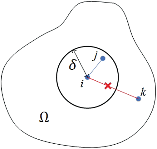
Figure 1: The interaction between material points

In bond-based peridynamics, the pair-wise force fij is dependent on the deformation of the bond between point i and j. The relative displacement vector η and initial relative position vector ξ are defined as:

η=u(xj,t)-u(xi,t) (2)

ξ=xj-xi (3)

The pair-wise force fij is linear with the bond’s stretch s:

fij=ω(|ξ|)⋅c⋅s⋅ξ+η|ξ+η| (4)

s=|ξ+η|-|ξ||ξ| (5)

where ω(|ξ|) denotes the distance influence function and equals to 1 in this study, c is the micro-modulus of the bond. The direction of fij is parallel with the deformed bond ξ+η, see Fig. 2a. The determination of micro-modulus c is by comparing the distribution of strain energy density between the peridynamics and continuum mechanics. The value of c is:

c={6Eπtδ3(1-μ)plane stress6Eπtδ3(1-2μ)(1-μ)plane strain6Eπδ4(1-2μ)3D(6)

where E is Young’s modulus, μ is the Poisson’s ratio, t is the thickness, δ is the horizon size.

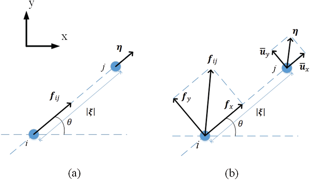
Figure 2: The pair-wise force: (a) Bond-based peridynamics, (b) Bond-based peridynamic model with rotation effect (BBPDR)

Because of the only one material parameter in bond-based peridynamics, there exists the limitation of Poisson’s ratio (μ=1/3 in plane stress, μ=1/4 in plane strain and 3D). To solve this problem, Silling et al. [46,47] develop the state-based peridynamic theories, including ordinary state-based peridynamics and non-ordinary state-based peridynamics. However, the state-based peridynamics are computing expensive and have the zero-energy mode. Considering the shortcomings of state-based peridynamics, the researchers develop the modified bond-based peridynamic models [48–51]. These modified bond-based peridynamic models extend the relation between peridynamic pair-wise force and relative deformation, which considers the rotations of material points and the tangential peridynamic pair-wise force.

The bond-based peridynamic model with rotation effect (BBPDR) is an extended model of the bond-based peridynamics [49]. In this model, the bond can transfer the pair-wise forces in both axial and tangential directions, see Fig. 2b. In isotropic elastic material, the number of material parameters in BBPDR is consistent with the one of continuum mechanics. And the numerical simulations of the paper [49] show that the limitation of Poisson’s ratio is solved. The axial pair-wise force fx and tangential pair-wise force fy is linear with the bond’s stretches in axial and tangential direction, respectively:

{fxfy}=[c00d]⋅{u¯x|ξ|u¯y|ξ|}(7)

where c and d are the micro-modulus in axial and tangential directions, u¯x and u¯y are the relative displacement components in axial and tangential directions. Similar to the method of determining the micro-modulus in bond-based peridynamics [45,56], c and d are determined by comparing the distribution of strain energy density between the BBPDR and the continuum mechanics. In the plane stress problem, the values of c and d are [49]:

{c=6Eπtδ3(1-μ)d=6E(1-3μ)πtδ3(1-μ2)(8)

Comparing Eq. (8) with Eq. (6), it shows that the micro-modulus in bond-based peridynamics is identical with the axial micro-modulus in BBPDR. When the fixed Poisson’s ratio μ=1/3 is applied, the tangential micro-modulus d equals 0 and the BBPDR degenerates into the bond-based peridynamics. This comparison shows that the bond-based peridynamics is a special case of BBPDR. Although the theoretical and numerical analysis of the paper [49] show that the BBPDR can solve the limitation of Poisson’s ratio, considering that the tangential stiffness d should be greater than 0 to avoid the negative work of tangential pair-wise force, the selection of Poisson’s ratio expands to -1<μ<1/3.

In peridynamics, the damage of material is described by bond breakage. The bond will break when its stretch s reaches its critical value sc, and the material with such character is called PMB (Prototype microelastic brittle) material [45]. Considering that concrete is a kind of brittle material, the assumption of PMB material is applied in this study. The scalar factor μ(t,ξ) is defined to show the bond’s breakage:

μ(t,ξ)={1s(t′)<sc,t′<t0otherwise(9)

where t′ is the time before the current time t. When the bond breaks, it cannot transmit interaction for material points anymore. sc is obtained by comparing fracture energy calculated in peridynamics and the critical energy release rate Gc. For simplicity, we only present the result in a plane stress problem [56]:

sc=4Gcctδ4(10)

where Gc is the critical energy release rate, c is the micro-modulus in bond-based peridynamics, t is the thickness, δ is the horizon size.

The damage value is defined as:

φ(xi,t)=1-∫Hiμ(t,ξij)dVj∫HidVj(11)

where φ(xi,t) is from 0 to 1, larger value means more broken bonds and more damage near the point i.

3  Fiber-Reinforced Concrete Model

Considering that the fiber content is low, and the fiber scale is small compared with the concrete matrix, a semi-discrete model is applied to model the fibers, see Fig. 3. Similar to the fiber modelling of paper [52,53], the fibers are not modelled independently, and the fiber reinforcement is implemented as the improvements of the bond’s strength and stiffness. Fig. 3 shows that the bonds passed by the fibers are enhanced, including the bond’s stiffness and strength, see Fig. 4.

E1=E0+ωf(|ξ|)⋅(Ef-E0) (12)

sc1=sc0+ωf(|ξ|)⋅(scf-sc0) (13)

where E1 and E0 are Young’s modulus of enhanced bond and normal bond respectively, ωf(|ξ|) is the influence function of a bond, which is chosen as ωf(|ξ|)=dx/|ξ| in this study, the smaller the distance between the material points and the fibers, the stronger the strengthening effect of fiber on the material points, Ef is the limit value of E1, sc1 and sc0 are the critical stretch of enhanced bond and normal bond respectively, scf is the limit value of sc1.

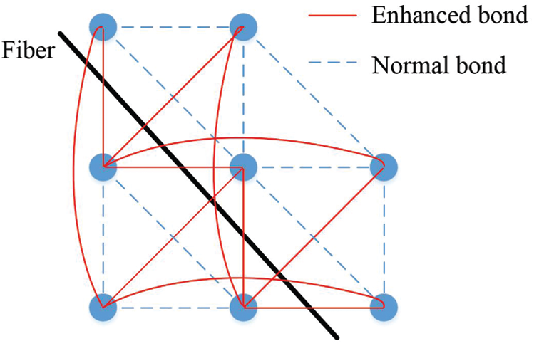
Figure 3: The bonds are enhanced by the fibers (δ=2dx)

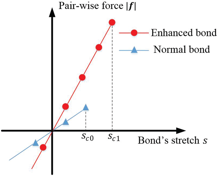
Figure 4: Fibers enhance the bond’s stiffness and strength

In this study, the frictional effect between fibers and the concrete matrix is considered. The frictional process starts when the damage value of the material points near the fiber reaches limit value φm:

max(φ(xi,t))≥φmxi∈Gf(14)

where xi is the location of point i, according to the paper [45], φm is chosen as 0.3, Gf is a group of material points, where the distance between the material points and the fiber is less than df, see Fig. 5. In this study, df equals 0.8⋅dx.

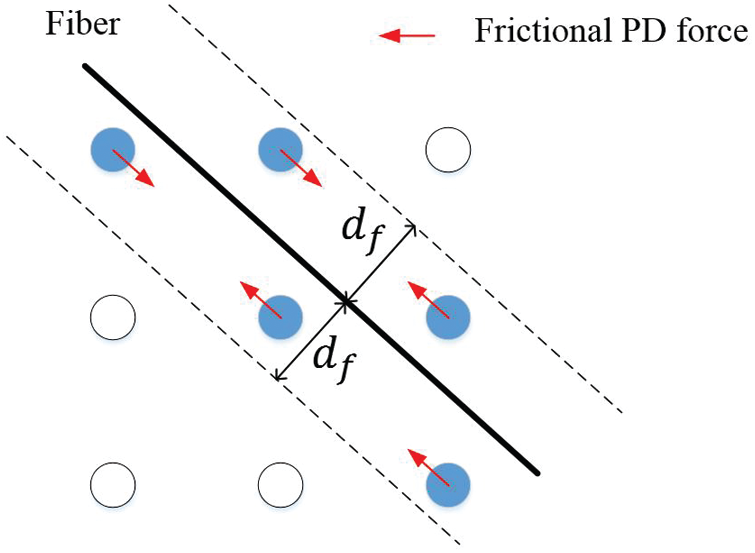
Figure 5: The influence range of the fiber

The frictional process is divided into two stages: Static friction and sliding friction, see Fig. 6. During the static friction (|u¯r|<u¯t), the frictional force density fr is linear with the relative displacement u¯r, which is calculated relative to the location when the friction process begins. During the sliding friction (|u¯r|≥u¯t), the frictional force density fr is a constant. The relation between fr and u¯r is:

fr={-kf⋅u¯r,|u¯r|<u¯t-kf⋅u¯t,|u¯r|≥u¯t(15)

where kf is the frictional stiffness, which is related to the interface properties between the fibers and concrete matrix, in this study, kf is calculated as:

kf=C⋅(c+d)⋅(dx)2(16)

where dx is the discretization grid size, C is a constant and equals 4000 (dx=1mm) and 2000 (dx=0.5mm), c and d are the micro-modulus in BBPDR, see Eq. (8). u¯t is the sliding limit of u¯r and equals sc⋅dx in this study.

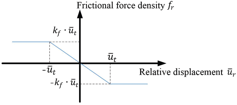
Figure 6: The relation between the frictional force density fr and relative displacement u¯r

Besides, the frictional force density is limited by Coulomb’s law of friction. The frictional force density cannot be greater than the limit value ft. When fr≥ft, fr equals to ft. The limit value of frictional force density is calculated as:

ft={cf⋅∑i=1nfi⋅ni⋅Viif∑i=1nfi⋅ni>00if∑i=1nfi⋅ni≤0(17)

where cf is the friction coefficient, n is the number of the enhanced bonds, fi is the pair-wise force of the enhanced bond, ni is the tangential direction vector of the fiber, ∑i=1nfi⋅ni⋅Vi calculates the compression between material point and fiber. The friction force density exists only when there is compression between the concrete and fibers.

The fibers are distributed randomly by using the “rand” function in MATLAB, and random numbers determine the center locations and angles of the fibers. In the actual situation, the fiber volume fraction is used to represent the fiber content in concrete, which is defined as Vf/V, where Vf is the total volume of fibers and V is the volume of the fiber-reinforced concrete. However, in the 2D plane stress problem, the fiber volume fraction calculated by Vf/V is relatively large because the thickness of the plate is small. Similar to the damage value of Eq. (11), the strengthening degree ei is used to represent the local fiber distribution near the region of point i, which is defined as:

ei=RiNi(18)

where Ri is the number of the enhanced bonds, Ni is the number of total bonds of the point i. The large strengthening degree means the dense distribution of the fibers near the material point.

4  Numerical Implementation

In peridynamics, the material domain is discretized into an assemble of material points to solve the Eq. (1) numerically. And the integration symbol of Eq. (1) is replaced with the summation notation. In this study, the discretization scheme of the material points is the uniform grid. Eq. (1) is rewritten as:

ρ(xi)⋅u¨(xi,t)=∑j=1nfij⋅nij⋅Vj+b(xi,t)(19)

where n is the number of the neighbors within the horizon, nij is the direction vector of the bond.

There are two widely used time integration methods in peridynamic numerical models: Explicit method and ADR method. In this study, the ADR method is applied to obtain the quasi-static solutions of Eq. (19). The same method is used in the papers [52–54], and the detailed discussions of the ADR method are made in paper [57] and book [56]. In the ADR method, the quasi-static solutions are obtained by adding the virtual damping force. The time step dt and the mass density are fictitious, dt equals 1.0 in this study. Eq. (19) is rewritten as:

M⋅U¨+C⋅U̇+P(U)+b(X)=0(20)

where M is the fictitious mass matrix and equals to mii⋅I, mii is the diagonal component of M and satisfied the inequality equation of Gerschgorin theorem [56], I is the identity matrix, U is the vector of displacements of all material points, C is the damping matrix and equals to cn⋅M, P is the vector of internal force density, b is the vector of body force density, X is the vector of the location of all material points. According to the book [56], mii is chosen as:

mii=14(dt)2⋅(πδ2tc)5dx(21)

where dt is the time step, t is the thickness of the plate, δ is the horizon size, dx is the discretization grid size.

The displacement vector U is obtained by applying the central time difference scheme:

U̇n+12=2-dt⋅cn2+dt⋅cnU̇n-12+2dt2+dt⋅cnM-1⋅(P(Un)+b(Xn)) (22)

Un+1=Un+dt⋅U̇n+12 (23)

U̇12=dt2M-1⋅(P(U0)+b(X0)) (24)

where n represents the nth step, and cn is calculated as:

cn=2(Un)T⋅P(Un)⋅Un(Un)T⋅M⋅Un(25)

Besides, there is a limit value of cn. When cn calculated by Eq. (25) is larger than 2.0, cn equals 1.9. Such limitation of cn guarantees numerical stability, and the numerical error is small.

5  Numerical Examples

In this section, four examples are simulated to validate the proposed model and analyze the fracture behavior of fiber-reinforced concrete, including the convergence study, the tensile test of a plate with a single fiber, the tensile test of a plate with two semi-circle notches, and the three-point bending beam test. In the first example, a static simulation of a square plate under tension is made to study the convergence of BBPDR. In the second example, a tensile test of the plate with a single fiber is simulated to validate the effectiveness of the proposed fiber-reinforced model. And in the following two examples, the specimens with randomly distributed fibers are tested. The results of the proposed model are contrasted with the numerical results of other models and the experimental results.

5.1 Convergence Study

A square plate under tension is tested to study the convergence of BBPDR, including the effects of discretization grid size dx and the horizon size δ on the numerical results. The geometry and boundary condition of the plate is shown in Fig. 7. The plate with dimension 100 mm×100 mm×1 mm is subjected to a displacement load at the top side, and its left and bottom side are fixed in x-direction and y-direction, respectively. Young’s modulus E is 210 GPa, and Poisson’s ratio μ is 0.2.

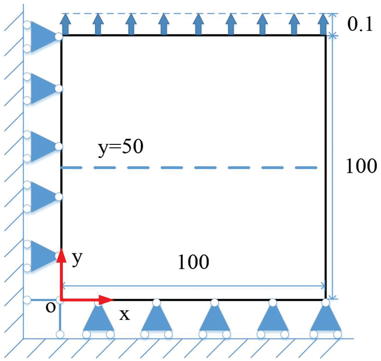
Figure 7: The geometry and boundary condition of the square plate under tension (unit: mm)

Eq. (19) is solved by an implicit scheme, which is detailed discussed in paper [51]. In the implicit scheme, the peridynamic integral equations are solved similar to the FEM, and the element stiffness matrix of a bond is obtained through the principle of virtual work.

Fig. 8 shows the x displacement distribution along the line y=50 mm (shown in Fig. 7) with different discretization grid sizes (dx = 1.0, 2.0, and 5.0 mm), and the horizon size δ equals 3.015⋅dx. Fig. 9 shows the x displacement distribution along the line y=50 mm with different horizon sizes (δ=2.0, 3.015, and 4.0 mm), and the discretization grid size dx is fixed as 1.0 mm. The numerical results are compared to the theoretical solution:

ut=-x⋅εy⋅μ(26)

where x is the x coordinate, εy is the strain in y-direction and equals 0.001, μ is the Poisson’s ratio. The relative error is calculated as:

er=|un-ut||ut|×100%(27)

where un are the numerical results.

Fig. 8 indicates that the numerical results converge to the theoretical solution as dx decreases. Fig. 9 shows that δ=3.015⋅dx has the highest accuracy, which is consistent with the suggestion of [56]. Too large or too small δ leads to errors in calculating the element stiffness matrix of a bond. The largest error appears at the left boundary because the x displacement is close to 0 at the region close to the left boundary. In the following examples, δ=3.015⋅dx is applied in all the examples. In the plate with a single fiber, dx = 1.0 mm is applied. And in the examples of crack propagation, dx = 0.5 mm is applied for high precision in predicting fracture behavior.

Figure 8: The x displacement along y=50 mm with different dx: (a) x displacement, (b) Relative error

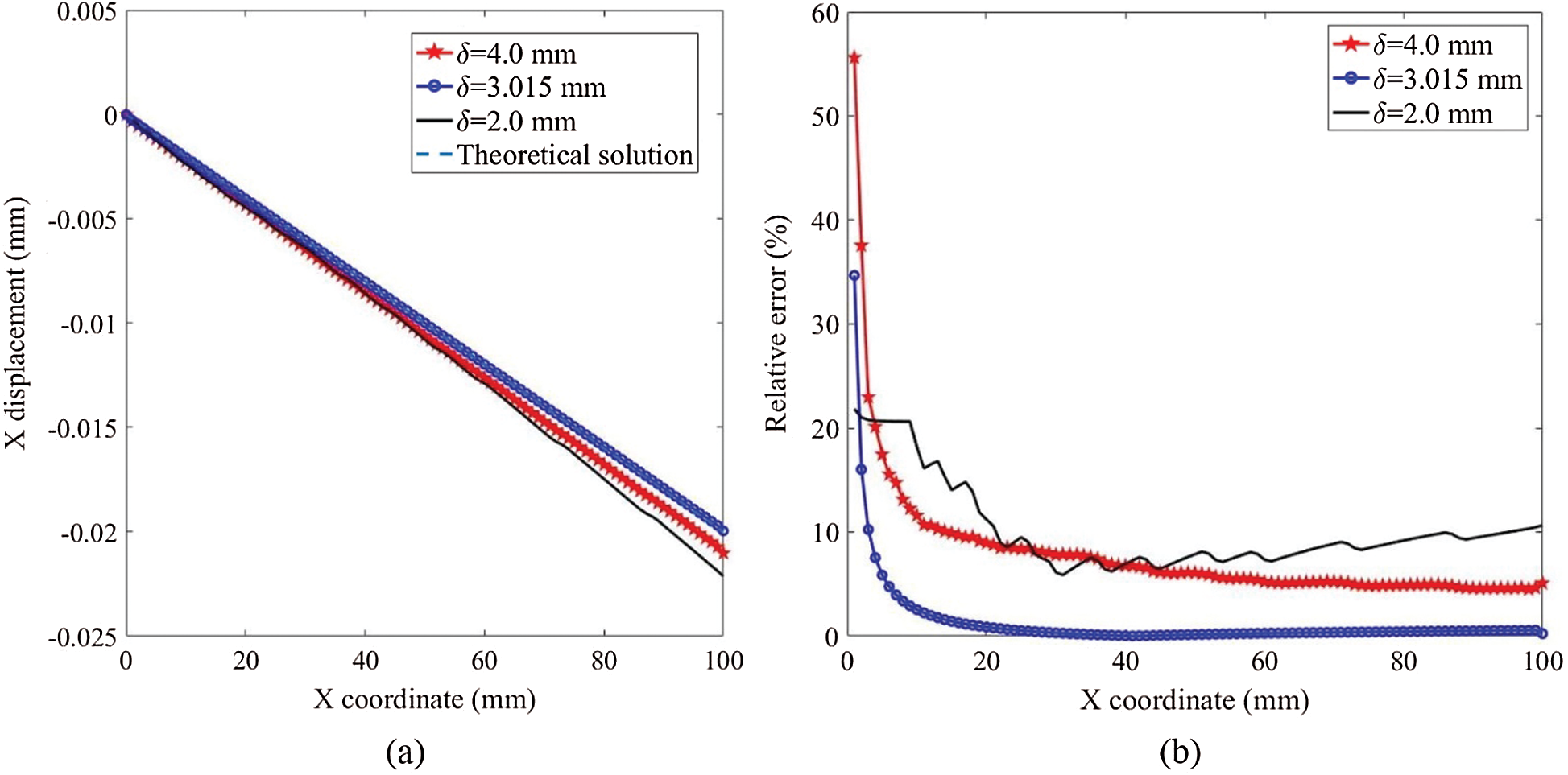
Figure 9: The x displacement along y=50 mm with different δ: (a) x displacement, (b) Relative error

5.2 Tensile Test of a Plate with a Single Fiber

In this section, the plate with a single fiber under tension is tested to validate the proposed fiber-reinforced model. The geometry and boundary condition of the plate is shown in Fig. 10. The plate with dimension 100 mm×20 mm×1 mm is subjected to a displacement load at the right side. The displacement load increases linearly with the time steps. The 60 mm fiber is located at the center of the plate, and a weak region with a width of 10 mm is defined at the center of the plate, see Fig. 10, where only the bonds connected to the points inside the weak region can break. The number of the material points is 2140, and the number of the total time step is 2000. Tab. 1 lists the mechanical parameters of the plate, where the Ef and scf are chosen greater than the E0 and sc0 to amplify the strengthening effect of fiber. A similar example with the same geometry condition is tested in the paper [52].

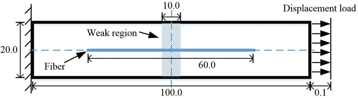
Figure 10: The geometry and boundary condition of the plate with a single fiber (unit: mm)

Table 1: Mechanical parameters of the plate with single fiber

The force-displacement load curves of the plain concrete and the fiber reinforced concrete are shown in Fig. 11. At the initial stage of loading (0–0.01 mm), the stress wave concentrates at the loading area, so the calculated reaction force remains zero. After the stress wave passes through the plate and reaches the left boundary, the calculated reaction force begins to rise. The tensile strength of the plate is increased by 11.5% and the ultimate strain is increased by 20% with the fiber reinforcement. Fig. 12 shows that the damage initiates at the right boundary of the weak region and passes through the plate. After adding the fibers, the path of crack changes to the direction along with the fiber, see Fig. 12b. Fig. 13 shows the strengthening degree of the material points (Fig. 13a) and the frictional force density (Fig. 13b). The strengthening degree is larger when the distance between the fiber and the material point becomes closer. The positive direction of the frictional force is defined as the direction of the load, see Fig. 13b. The frictional force densities are distributed on the material points close to the fiber, and the directions of frictional force densities are opposite on the two sides of the crack surface, see Fig. 13b. Hence, the material points tend to move toward the crack surface, and the crack propagation near the fiber is prevented.

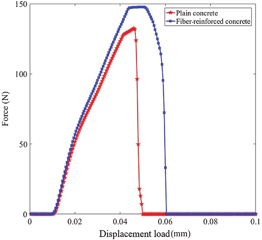
Figure 11: The force-displacement load curves of the plates under tension

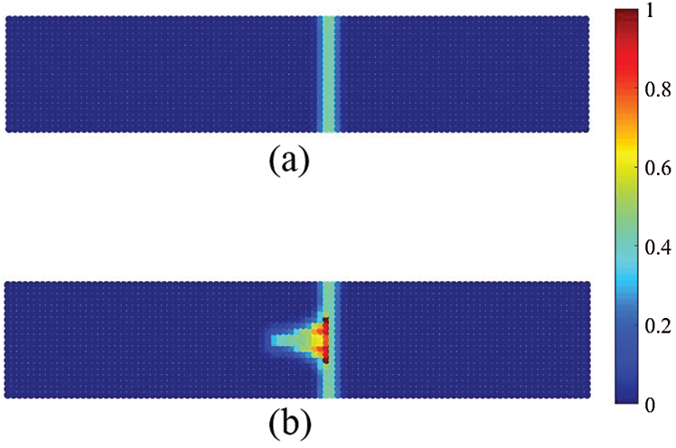
Figure 12: The crack paths of the plates under tension: (a) Plain concrete, (b) Fiber-reinforced concrete

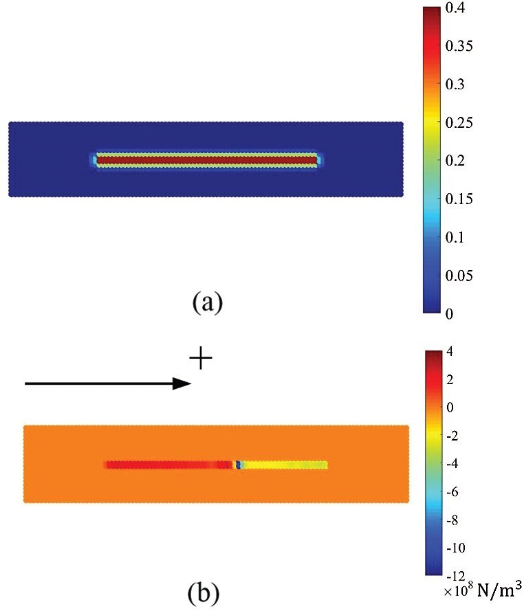
Figure 13: The distribution of the strengthening degree (a) and the frictional force density along the fiber (b)

The influence of the frictional coefficient cf is investigated and four different frictional coefficients are chosen, cf = 0.1, 0.3, 0.7, 0.9. The frictional coefficient describes the frictional characteristics of the fiber, which is related to the fiber formation and fiber type. Fig. 14 shows the comparison of force-displacement load curves with different frictional coefficients. With the increase of frictional coefficient, the descending parts of the force-displacement load curves become slower, and the toughnesses of the plates become greater. However, the frictional coefficient has little effect on tensile strength.

Figure 14: The force-displacement load curves of the plate with different frictional coefficients

Besides, the proposed model is compared with the numerical model of fiber-reinforced concrete in paper [54]. For simplicity, the numerical model of paper [54] is named as the random bond model in the following discussions. In the random bond model, the bond-based peridynamics is applied to calculate the pair-wise force between the material points, see Eq. (4), and the strengthening effect of the fiber is implemented by a randomly distributed PVA-fiber bond. This relation is similar to the fiber’s strengthening effect of the proposed model, see Fig. 4. The stiffness and critical stretch of the PVA-fiber bond are higher than the concrete bond. And the fiber volume fraction is defined as:

Rv=LfiberLall(28)

where Lfiber is the sum of lengths of all the PVA-fiber bonds, Lall is the sum of lengths of all the bonds. The fiber volume fraction determined by Eq. (28) is influenced by horizon size δ, and Rv decreases when δ rises.

The tensile test setup is the same as Fig. 10. Different from the fiber modelling of the proposed model, the fiber in the random bond model is represented by randomly distributed PVA-fiber bonds. Fig. 15 shows the distribution of PVA-fiber bonds, and the volume fraction equals 20.26%, which is higher than the common cases (0.25%–2%). This example is only used to compare the proposed model and the random bond model, which is not of practical significance. The mechanical parameters of the random bond model are listed in Tab. 2. The mechanical parameters of the proposed model are similar to Tab. 1 and only the frictional coefficient cf is changed to 0.9.

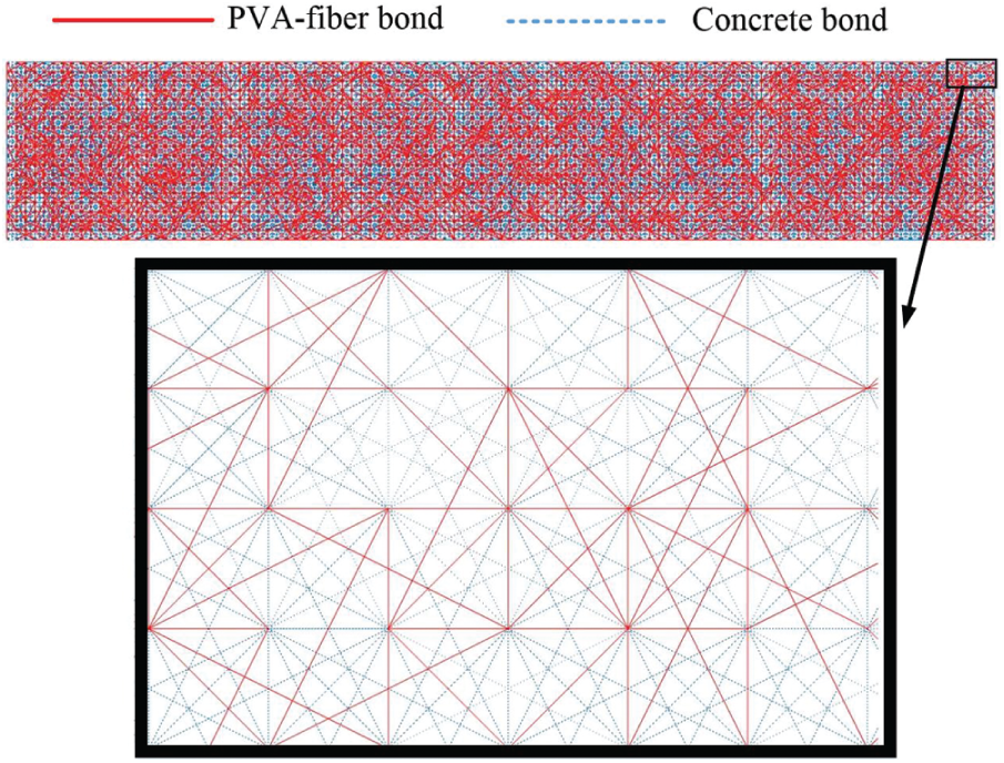
Figure 15: The distribution of PVA-fiber bonds in the random bond model

Table 2: Mechanical parameters of the random bond model

Fig. 16 shows the force-displacement load curves of plain concrete and fiber-reinforced concrete. Since the random bond model is developed based on the bond-based peridynamics, the tensile test of plain concrete is also simulated by using the bond-based peridynamics. The two curves of the plain concrete are almost the same. And the descending part of the random bond model is characterized by brittle fracture.

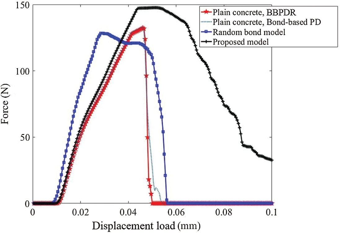
Figure 16: The force-displacement load curves of different models

To further investigate the reinforcement effect of the random bond model, the plates with the different critical stretch of PVA-fiber bond scf are simulated. Fig. 17 shows the force-displacement load curves with four different scf (scf=1.0×10-3, 1.2×10-3, 1.5×10-3, 1.8×10-3). The tensile strength increases as scf increases, but the brittle fracture that occurs at the descending parts remains the same. Fig. 18 shows the force-displacement load curves of the proposed model with four different scf (scf=2.2×10-3, 2.4×10-3, 2.8×10-3, 3.0×10-3). Because of the low content of the enhanced bond, see Figs. 10 and 13a, in the proposed model, scf has little effect on the tensile strength but slows down the descending part of the force-displacement load curve. The toughness of the plate becomes greater with higher scf.

Figure 17: The force-displacement load curves of the random bond model with different scf

Figure 18: The force-displacement load curves of the proposed model with different scf

The results shown in Figs. 16–18 indicate that the random bond model is capable of simulating the strengthening effect of fibers, but hard to simulate the improvement of toughness. Besides, the limitation of Poisson’s ratio in bond-based peridynamics may lead to numerical errors when simulating the fiber-reinforced concrete (μ=0.2). The proposed model is developed based on the BBPDR, which expands the selection of Poisson’s ratio (-1<μ<1/3). Both the strengthening effect and toughness improvement can be simulated by the proposed model, see Figs. 11–14. And the semi-discrete fiber modelling shows the distribution of fibers more comprehensively.

5.3 Tensile Test of a Plate with Two Semi-Circle Notches

In paper [52], the tensile tests of a plate with two semi-circle notches are simulated to illustrate the effect of fiber volume fractions on tensile strength. The geometry and boundary condition of the plate is shown in Fig. 19. The plate with two symmetry semi-circle notches is subjected to a displacement load. The mechanical parameters are shown in Tab. 3. The selection of parameters and the geometry condition are referred to as paper [52]. The number of the material points of the plate is 8153, and the number of the total time steps is 20000.

Figure 19: The geometry and boundary condition of the plate with two semi-circle notches (unit: mm)

Table 3: Mechanical parameters of the plate with two semi-circle notches

As discussed in Section 3, the fiber volume fraction is replaced with the strengthening degree to characterize the fiber content. Fig. 20 shows the distributions of fibers of the plate. Two different numbers of fibers (100 fibers and 200 fibers) are applied, and the fiber volume fractions are defined as α and 2α, respectively. The strengthening degree of the plate with a higher fiber volume fraction is distributed more intensively.

Figure 20: The fiber distributions of the plate with a circular notch: (a) vf=α (100 fibers), (b) vf=2α (200 fibers)

Fig. 21 shows the force-displacement load curves of the plate with different fiber volume fractions. After adding the fibers, the tensile strengths of the plates are increased by 9.7% (vf=α) and 23.6% (vf=2α) relative to the plain concrete. Different from the brittle fracture of the plain concrete, the descending parts of the fiber reinforced concrete are characterized by the ductile fracture. Fig. 22 shows the crack path of the plate with different fiber volume fractions, and the results are compared with the paper [52]. The crack path is not a straight line after adding the fibers, but the damaged area is still in the center part of the plate. The fibers have a slight effect on the crack propagation but do not change its main direction.

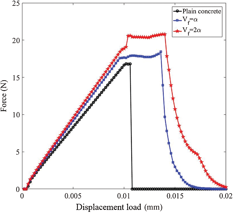
Figure 21: The force-displacement load curves of the plate with different fiber volume fraction

Figure 22: The crack propagation of the plate with different fiber volume fraction: (a) Plain concrete, (b) vf=α, (c) vf=2α, (d) Fiber-reinforced concrete, vf=0.6% [52]

Besides, the influence of fiber distribution on crack propagation is investigated. As reported in paper [9], the strengthening effect of fibers is maximized when the fibers are aligned perpendicular to the crack path. In this example, four different fiber distribution with vf=α are selected, named as (a), (b), (c), and (d). The strengthening degrees of four different fiber distributions are shown in Fig. 23. Fig. 24 shows the force-displacement load curves of the plate with different fiber distributions. The tensile strength of the plate is slightly influenced, and the fiber distribution mainly influences the descent part of the curves. The curves of distribution (b) and distribution (c) descend more slowly than the other two fiber distributions. This phenomenon results from the concentration of fibers in the center part of the plate. Figs. 23 and 25 show that the strengthening degrees in the center part (|x|<2.5 mm) of distribution (b) and distribution (c) are higher than the other two fiber distributions. The plate with a higher strengthening degree in the center part shows greater toughness in the tensile test. Although the strengthening effect of fiber distribution and fiber agglomeration on concrete is complex, the strengthening degree defined by Eq. (18) can characterize the fiber reinforcement effect to a certain degree. Fig. 26 shows the crack paths of different fiber distributions. The fiber distribution influences the local damage, but the damages still mainly concentrate in the center of the plate.

Figure 23: The strengthening degree of the plate with four different fiber distribution, and the total strengthening degrees located at center region are shown in Fig. 25: (a) 156.1, (b) 190.8, (c) 198.6, (d) 150.9

Figure 24: The force-displacement load curves of the plate with four different fiber distributions

Figure 25: The total strengthening degree of the material points located at the center region (|x|<2.5 mm)

Figure 26: The crack paths of the plate with four different fiber distributions, and the total strengthening degrees located at center region are shown in Fig. 25: (a) 156.1, (b) 190.8, (c) 198.6, (d) 150.9

5.4 Three-Point Bending Beam Test

This section discusses a three-point bending beam test. The geometry and boundary condition of the beam is shown in Fig. 27. The final central deflection is 0.25 mm. The beam has a dimension of 160 mm×40 mm×0.5 mm with a notch of 18 mm. The number of the material points of the beam is 26019. The notch location is changed with c=0, 20, 40 mm. As the notch location changes, the crack pattern changes from the pure mode I to the mixed mode of Mode I and Mode II. The mechanical parameters are shown in Tab. 4. The selection of the mechanical parameters is referred to as paper [54]. Fig. 28 shows the distribution of fibers and the number of fibers is 100. The number of total time steps is 40000.

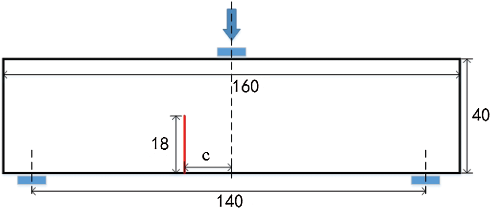
Figure 27: The geometry and boundary condition of the three-point bending beam test (unit: mm)

Figure 28: The distribution of fibers of the three-point bending beam test

Table 4: Mechanical parameters of the three-point bending beam test

Fig. 29b shows the crack path of the proposed model with c=0 mm. The crack pattern is the pure mode I, and the crack propagates along the centerline of the beam. Comparing with the results of plain concrete, see Fig. 29a, the crack path has some perturbation because of the fibers. As discussed in the previous sections, the addition of fibers does not change the main direction of the crack path but influence the local damage distribution. The results match well with the experiments of paper [54], see Fig. 29c. Fig. 30 shows the deflection-force curves of plain concrete and fiber reinforced concrete. At the initial stage of the loading (0–0.01 mm), the calculated reaction force is zero or less than zero. Because the stress wave concentrates at the loading area, and the stress wave reflection occurs at the bottom boundary. After the stress wave reaches the bottom boundary (0.01–0.05 mm), the calculated reaction force begins to rise. The flexural strength of the beam is increased by 26.2% after adding fibers. When the curves approach the peak value (0.05–0.13 mm), the vibration of the curves becomes severe. And the same phenomenon appears during the descending part (0.13–0.25 mm). The crack influences the stress wave propagation, which leads to the oscillation phenomenon of the reaction force. Fig. 31 shows the deflection-CMOD (Crack Mouth Opening Displacement) curves of plain concrete and fiber reinforced concrete. After the deflection reaches 0.08 mm, the CMOD of fiber reinforced concrete is lower than the one of plain concrete, which indicates that the fiber inhibits the crack opening process.

Figure 29: The crack path of three-point bending beam (c=0mm): (a) Plain concrete, (b) Fiber-reinforced concrete, (c) Fiber-reinforced concrete [54]

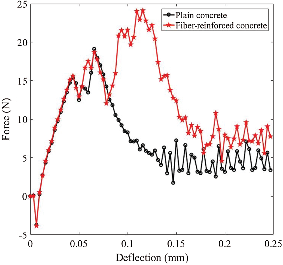
Figure 30: Deflection-force curves of three-point bending beam (c=0 mm)

Figure 31: Deflection-CMOD curves of three-point bending beam (c=0 mm)

When the notch location is off-center, the crack pattern is the mixed mode of Mode I and Mode II. Figs. 32 and 33 show the crack propagation of the beams with c=20 mm and c=40 mm. In Fig. 33, the crack path of the fiber reinforced concrete with c=40 mm is different from the experimental results. This difference results from the different local fiber distribution and the Poisson’s ratio. The experimental results of the paper [8] show that the oblique angles of cracks are different when the beam is prepared with different fiber volume fractions. And the numerical results of papers [53,54] show that the oblique angles of cracks are different from the experimental results when the fiber distributions are different. Fig. 34 shows the crack path of fiber-reinforced concrete with μ=0.29, which is similar to the experimental results shown in Fig. 33c. Poisson’s ratio influences the ratio of the axial stiffness and the tangential stiffness, see Eqs. (7) and (8). Considering that the effect of Poisson’s ratio on crack propagation is not the objective of this study, only the simulated results with μ=0.29 are shown. Figs. 35 and 36 show the deflection-force curves of the three-point bending beams with c=20 mm and c=40 mm. The flexural strengths of the beams with different notch locations are increased by 52.2% (c=20 mm) and 25.6% (c=40 mm) after adding fibers.

Figure 32: The crack path of three-point bending beam (c=20 mm): (a) Plain concrete, (b) Fiber-reinforced concrete, (c) Fiber-reinforced concrete [54]

Figure 33: The crack path of three-point bending beam (c=40 mm): (a) Plain concrete, (b) Fiber-reinforced concrete, (c) Fiber-reinforced concrete [54]

Figure 34: The crack path of three-point bending beam with Poisson’s ratio μ=0.29

Figure 35: Deflection-force curves of three-point bending beam (c=20 mm)

Figure 36: Deflection-force curves of three-point bending beam (c=40 mm)

6  Discussion and Conclusion

This paper proposes a peridynamic fiber reinforced concrete model based on the bond-based peridynamic model with rotation effect (BBPDR). The fiber is modelled in a semi-discrete way, and the fiber reinforcement is implemented by the improvements of bonds’ strength and stiffness. In the proposed model, the friction interaction between fibers and the concrete matrix is considered, which is divided into static friction and slip friction.

Numerical examples validate the proposed model’s effectiveness in modelling the fracture behavior of fiber-reinforced concrete. After adding the fibers, the tensile strength, flexural strength, and toughness of the concrete are improved. The fibers influence the path of crack propagation and the descending part of the load-deflection curve. The numerical results of the proposed model are compared with the experimental results and numerical results of other numerical models. And the comparisons show the effectiveness and validation of the proposed model in simulating the fracture behavior of fiber-reinforced concrete.

In future work, the authors will investigate the corresponding relation between the numerical parameters and the physical properties of the fiber. And the optimization analysis of the fiber distribution and the hybrid fiber combination will be studied, which helps design the fiber-reinforced concrete with better performance.

Acknowledgement: The authors thank the editors and the reviewers for their suggestions.

Funding Statement: The authors are pleased to acknowledge the support by the National Natural Science Foundation of China through contract/Grant Nos. 11772237, 11472196 and 11172216, and to acknowledge the open funds of the State Key Laboratory of Structural Analysis for Industrial Equipment (Dalian University of Technology) through contract/Grant No. GZ19110.

Conflicts of Interest: The authors declare that they have no conflicts of interest to report regarding the present study.

This work is licensed under a Creative Commons Attribution 4.0 International License, which permits unrestricted use, distribution, and reproduction in any medium, provided the original work is properly cited.