| Computer Modeling in Engineering & Sciences |
DOI: 10.32604/cmes.2021.014174
ARTICLE
Multi-Criteria Decision Making Based on Bipolar Picture Fuzzy Operators and New Distance Measures
1Department of Mathematics, University of the Punjab, Lahore, 54590, Pakistan
2School of Mathematics, Thapar Institute of Engineering and Technology (Deemed University), Patiala, 147004, India
3Algebra and Applications Research Unit, Division of Computational Science, Faculty of Science, Prince of Songkla University, Hat Yai, Songkhla, 90110, Thailand
4Centre of Excellence in Mathematics, Bangkok, 10400, Thailand
*Corresponding Author: Ronnason Chinram. Email: ronnason.c@psu.ac.th
Received: 06 September 2020; Accepted: 21 December 2020
Abstract: This paper aims to introduce the novel concept of the bipolar picture fuzzy set (BPFS) as a hybrid structure of bipolar fuzzy set (BFS) and picture fuzzy set (PFS). BPFS is a new kind of fuzzy sets to deal with bipolarity (both positive and negative aspects) to each membership degree (belonging-ness), neutral membership (not decided), and non-membership degree (refusal). In this article, some basic properties of bipolar picture fuzzy sets (BPFSs) and their fundamental operations are introduced. The score function, accuracy function and certainty function are suggested to discuss the comparability of bipolar picture fuzzy numbers (BPFNs). Additionally, the concept of new distance measures of BPFSs is presented to discuss geometrical properties of BPFSs. In the context of BPFSs, certain aggregation operators (AOs) named as “bipolar picture fuzzy weighted geometric (BPFWG) operator, bipolar picture fuzzy ordered weighted geometric (BPFOWG) operator and bipolar picture fuzzy hybrid geometric (BPFHG) operator” are defined for information aggregation of BPFNs. Based on the proposed AOs, a new multi-criteria decision-making (MCDM) approach is proposed to address uncertain real-life situations. Finally, a practical application of proposed methodology is also illustrated to discuss its feasibility and applicability.
Keywords: Bipolar picture fuzzy set; aggregation operators; distance measures; pattern recognition; MCDM
In any real-life problem-solving technique, the complexity characterizes the behavior of an object whose components interrelate in multiple ways and follow different logical rules, meaning there is no fixed rule to handle multiple challenges due to various uncertainties in real life circumstances. Many scholars from all over the world have apparently studied MCDM management techniques extensively. This effort resulted in a multitude of innovative solutions to complex real concerns. The frameworks for this objective are largely based on a summary of the issues at hand. To deal with uncertainties the researchers have been proposed various mathematical techniques. Zadeh [1] initiated the idea of fuzzy set (FS) and membership degrees of objects/alternatives. Later, the intuitionistic fuzzy set (IFS) proposed by Atanassov [2] is the direct extension of FS by using membership degrees (MDs) and non-membership degrees (NMDs). Yager et al. [3,4] and Yager et al. [5] introduced Pythagorean fuzzy set and Pythagorean fuzzy membership grades. Zhang et al. [6,7] introduced an independent extension of fuzzy set named as bipolar fuzzy sets (BFSs) and Lee [8] presented some basics operations. A bipolar fuzzy information is used to express a property of an object as well as its counter property.
Alcantud et al. [9] initiated the notion of N-soft set approach to rough sets and introduced the concept of dual extended hesitant fuzzy sets [10]. Akram et al. [11,12] initiated MCDM based on Pythagorean fuzzy TOPSIS method and Pythagorean Dombi fuzzy AOs. Ashraf et al. [13] initiated spherical fuzzy Dombi AOs. Eraslan et al. [14] and Feng et al. [15] proposed new approaches for MCDM. Garg et al. [16–18] introduced some AOs on different sets also their applications to MCDM. Jose et al. [19] proposed AOs for MCDM. Karaaslan [20], Liu et al. [21], Liu et al. [22], Wang et al. [23], Yang et al. [24], Smarandache [25], and Liu et al. [26] initiated many different approaches including AOs on different extension of fuzzy set for MCDM. Naeem et al. [27,28], Peng et al. [29,30], Peng et al. [31] introduced some significant results for Pythagorean fuzzy sets.
Riaz et al. [32], initiated the concept of linear Diophantine fuzzy Set and its applications to MCDM. Riaz et al. [33] introduced some hybrid AOs, Einstein prioritized AOs [34], related to q-ROFSs. Riaz et al. [35] introduced cubic bipolar fuzzy set and related AOs. Cagman et al. [36], and Shabir et al. [37] independently introduced the notion of soft topological spaces.
Cuong [38] presented the idea of a picture fuzzy set (PFS) as a new paradigm distinguished with three functions that assign the positive membership degree (MD), the neutral MD and the negative membership degree (NMD) to each object/alternative. The basic restrictions on these degrees are that they lie in [0, 1] and their sum also lies in [0, 1]. Cuong [39] further introduced the concept of Pythagorean picture fuzzy sets and its basic notions. Garg [40], Jana et al. [41] and Wang et al. [42] proposed some AOs for picture fuzzy information aggregation. Pamucar [43] studied the notion of normalized weighted geometric Dombi Bonferoni mean operator with interval grey numbers: Application in multicriteria decision making. Pamucar et al. [44] proposed an application of the hybrid interval rough weighted Power-Heronian operator in multi-criteria decision making. Ramakrishnan et al. [45] introduced a cloud TOPSIS model for green supplier selection. Riaz et al. also introduced some AOs [46,47] related to green supplier selection. Si et al. [48] and Sinani [49] also presented different AOs in some extension of fuzzy set.
The first objective of this paper is to introduce bipolar picture fuzzy sets (BPFSs) as a new hybrid structure of bipolar fuzzy sets (BFSs) and picture fuzzy sets (PFSs). BPFSs are more efficient for dealing with the real-life situation when modeling needs to address the bipolarity (both positive and negative aspects) to each MD (belonging-ness), neutral membership (not decided), and non-membership degree (refusal). The second objective of BPFSs is propose bipolar picture fuzzy MCDM technique based on bipolar picture fuzzy AOs. The third objective of BPFSs is to define new distance measure and its application towards pattern recognition. Additionally, the proposed methodology can extend to solve various problems of artificial intelligence, computational intelligence and MCDM that involve bipolar picture fuzzy information.
The rest of the paper is as follows. The definitions of IFS, PFS and BFS are discussed in Section 2. Section 3 introduces the definition of BPFS. Section 4 indicates some bipolar picture AOs and new BPFS distance measures. Section 5 shows the generalizability of the suggested paradigm for pattern recognition. Section 6 introduces a new BPF-MCDM approach based on suggested AOs and a numerical example. Finally, Section 7 summarizes the findings of this research study.
In this section, we give some basic definitions to IFSs, BFSs and PFSs.
Definition 2.1 [2] Let
where
Definition 2.2 [38] Let
where,
A basic element
Definition 2.3 [38] Some operational laws of picture fuzzy set as follows:
Let
1.
2. P1 = P2 iff,
3. The complement of P1 is defined by
4. The union is defined by
5. The intersection is defined by
Definition 2.4 [40] The score function of a PFN
However, in certain circumstances, the previous score function may not rank any two PFNs. For example, P1 = (0.7, 0.2, 0.1) and P2 = (0.6, 0.1, 0.1) then they have same score function values, i.e., R(P1) = R(P2). For this we use accuracy function given as
Let
1. If R(P1) > R(P2), then P1 > P2.
2. If R(P1) = R(P2), then,
If
If
Definition 2.5 [6] Let X be a set, a BFS B inX is defined as follows:
where
Definition 2.6 [6,7] Some operational laws of bipolar fuzzy set as follows:
Let
1.
2. B1 = B2 iff,
3. The complement of B1 is denoted by
4. The union is defined by
5. The intersection is defined by
6.
Here,
7. Support (
Here,
The BFS assign positive and negative grades to the alternatives and PFS is characterized by three functions expressing the MD, the neutral MD and the NMD. Fuzzy set assign a membership grade to each alternatives
We present the idea of BPFS as a new hybrid version of BFS and PFS. In this model of BPFS, we assign positive and negative grades for each MD (belonging-ness), neutral membership (not decided), and non-membership degree (refusal). We present specific examples to relate the proposed model with the real life applications. We define some operational laws of BPFS along with its score and accuracy functions.
Definition 3.1 A BPFS
where
The positive MDs
Now we discuss some applications of proposed model to relate it with real life problems.
Business:
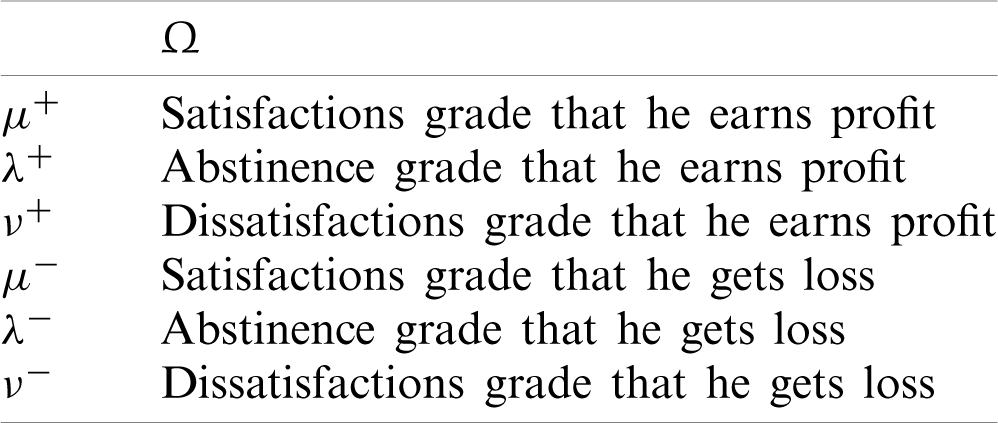
In the field of finance and business, we use two terms profit and loss. We can relate the decision-making applications based on business with BPFS. If a person invests some money, then he wants to earn max profit in some interval of time. Bipolar picture fuzzy number (BPFN) can be described as
The physical meaning of this structure in business terms is that, what is the satisfactions grade that he earns profit
Table 1: Tabular representation of BPFN under business related problems
Medication:
In the field of medical, we mostly focus on the effects and side effects of medicines related to every disease. If a patient get some medication according to his type of disease, then we can relate our model to the effects and side effects of that medicine in medical diagnosis, treatment and recovery terms. For the BPFN can be written as
Table 2: Tabular representation of BPFS under medical related problems
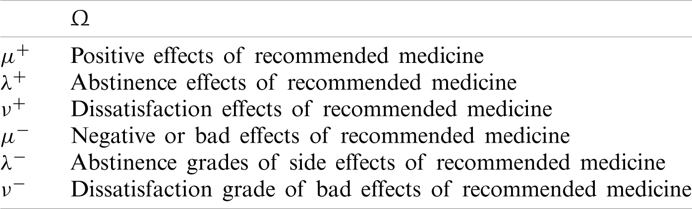
The proposed model is superior than these two models, in fact it is hybrid structure of BFS and PFS that assign six grades to the alternative.
Comparison Analysis:
In this part, we discuss about the terms and characteristics of proposed model and compare it with the existing techniques. There are various objectives to construct this hybrid structure and some of them are listed below:
1. The first objective to construct this hybrid model is to fill the research gap which exists in previous methodologies. The bipolar fuzzy set and picture fuzzy set can be used together in decision analysis. We can deal with the satisfaction, abstinence and dissatisfaction grades of the alternatives with its counter properties.
2. The second objective is that we can cover the evaluation space in a different manner. If we compare our model with the existing theories then we find that it is strong, valid and superior to others. The comparison analysis of BPFS with the existing models is given in Tab. 3.
3. The third objective is to represent the relationship of BPFS to the MCDM problems. We study some real life problems and convert the input data into BPF numeric values and deal it with the proposed aggregation operators. This novel structure is superior, flexible and easy to handle and can deal with the MCDM problems in the field of medical, business, artificial intelligence and engineering etc. The graphical representation of PFS and BPFS is given in the Figs. 1 and 2, respectively.
4. In bipolar neutrosophic set (see [50]) the conditions are as follows:
However, in the proposed model BPFS the conditions are as follows:
Table 3: Comparison of BPFS with the existing set theoretic models
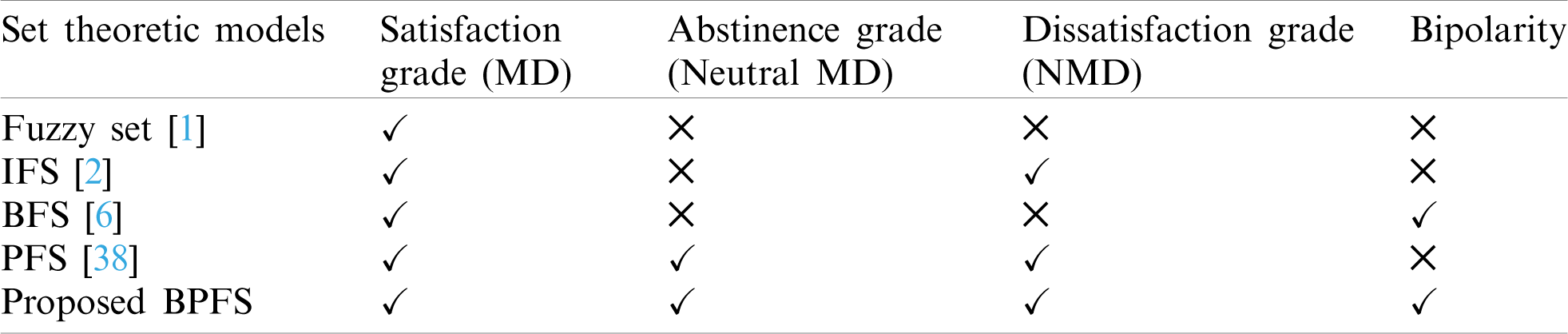
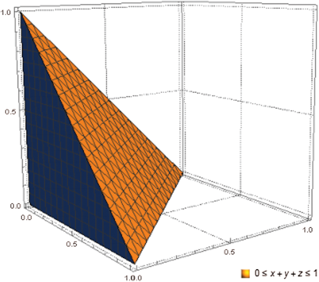
Figure 1: Graphical representation for satisfaction, abstinence and dissatisfaction grades of picture fuzzy set.
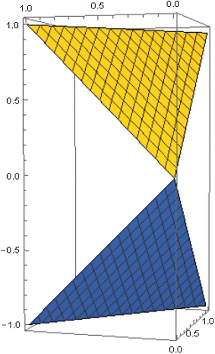
Figure 2: Graphical representation for grades of bipolar picture fuzzy set
Definition 3.2 Let
Definition 3.3 Let
and
Definition 3.4 Let
The union of these two
Example 3.5 Let
Then their union is
Definition 3.6
The intersection of these two
Example 3.7 Let
Then their intersection is
Definition 3.8 Let
Example 3.9 Let
Then its complement is
Now we see that BFS and PFS are special cases of BPFS.
Proposition 3.10 BFS and PFS are special cases of BPFS, i.e., Bipolar fuzzy numbers (BFNs) and picture fuzzy numbers (PFNs) are special cases of the bipolar picture fuzzy numbers (BPFNs).
Proof. For any
Similarly, by setting the components
Theorem 3.11 Let
1.
2.
3.
4.
5.
6.
7.
8.
9.
10.
Proof. The proof is obvious.
Theorem 3.12 Let O and P be the BPFSs in a universe X, then we have
1.
2.
We will denote the set of all
Definition 3.13 Let
1.
2.
3.
4.
5.
4 Some Bipolar Picture Fuzzy Geometric Operators
In this section, firstly, we introduce score function, accuracy function, and certainty function for BPFNs. Secondly, we introduce BPFWG operator, BPFOWG operator, and BPFHG operator.
Definition 4.1 Let
1.
2.
3.
The range of score function
Definition 4.2 Let
1. if
2. if
3. if
4. if
Definition 4.3 Let
Theorem 4.4 Let
Proof. Using mathematical induction to prove this theorem.
For n = 2
Then, it follows that
This shows that it is true for n = 2, now let that it holds for n = k, i.e.,
Now n = k + 1, by operational laws of BPFNs we have
This shows that for n = k + 1, holds. Thus, by the principle of mathematical induction Theorem 4.4 holds for all n.
Below we define some of
Theorem 4.5 (Idempotency) Let
Proof. Since,
We know,
Theorem 4.6 (Monotonicity) Let
Proof. Here, we omit the proof.
Example 4.7 Let T1, T2, T3, T4 be the BPFNs as follows:
and P = (0.3, 0.2, 0.1, 0.4) then
When we need to weight the ordered positions of the bipolar picture fuzzy arguments instead of weighting the arguments themselves,
Definition 4.8 Let
where Pj is the WV of
According to the operational laws of the BPFNs, we can obtain the following theorems. Since their proofs are similar to those mentioned above, we are omitting them here.
Theorem 4.9 Let
Theorem 4.10 (Idempotency) Let
Theorem 4.11 (Monotonicity) Let
Theorem 4.12 (Commutativity) Let
where
When both the ordered positions of the bipolar picture fuzzy arguments and the arguments themselves need to be weighted, BPFWG can be generalized to the following bipolar picture fuzzy hybrid geometric operator.
Definition 4.13
We can drive the following theorem based on the operations of the PFNs which is similar to Theorem 4.4.
Theorem 4.14
The weighting vector associated with the operator of BPFWG, the operator of BPFOWG and the operator of BPFHG can be assessed as identical to that of the other operators. For example, a normal distribution-based approach can be used to evaluate weights. The distinctive feature of the approach is that it can reduce the effect of bias claims on the outcome of the judgment by assigning low weights to the wrong ones.
4.1 Distance Measure of Bipolar Picture Fuzzy Sets
In this section of the paper, we define the distance measures of bipolar picture fuzzy sets.
Definition 4.15 A function
1.
2.
3.
Theorem 4.16
We can actually confirm that the functions in Theorem 4.16 satisfy distance measuring properties between bipolar picture fuzzy sets. In it,
Example 4.17 Assume there are three patterns denoted by BPFSs on
are three bipolar picture fuzzy set in X. Using Theorem 4.16, we get
and
5 MCDM Based on BPFS to Pattern Recognition
In this section, we discuss some distance measures of BPFSs and their application to the pattern recognition. Pattern recognition is a science and technology discipline which aims to classify objects into a number of categories. This method is widely used in the identification of data analysis, shapes, pattern classification, traffic analysis & regulation, natural language processing, rock identification, biological stimuli, odor identification, understanding of the DNA sample, credit fraud detection, biometrics including fingerprints, palm vein technology & face recognition, medical diagnosis, weather forecasting, intelligence, informatics, voice to text transition, terrorism identification, radar tracking, and automatic military target recognition, etc. In Fig. 3 step by step method is shown of facial recognition which is example of pattern recognition.
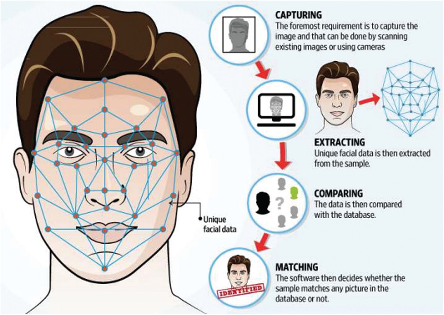
Figure 3: Method of facial recognition
5.1 Numerical Example for Using New Measures in Pattern Recognition
Example 5.1 Suppose that there are three patterns denoted by BPFSs on
Now, there is a sample,
The question is, what pattern belongs to B? By applying the distance measure
We see that B belongs to pattern
6 MCDM Based on Some Bipolar Picture Fuzzy Geometric Operators
MCDM method using the aggregation operators defined for BPFNs is presented in this section.
Suppose that
1.
2.
Indeed an algorithm is being developed to discuss MCDM.
Algorithm
Step 1.
The DM has given its personal opinion in the form of BPFNs.
Step 2.
Normalize the decision matrix. If there are different types of criteria or attributes like cost and benefit. By normalize the decision matrix we deal all criteria or attributes in the same way. Otherwise, different criterion or attributes should be aggregate in different ways.
where
Step 3.
Based on decision matrix acquired from Step 2, the aggregated value of the alternative Ti under various parameter Cj is obtained using either BPFWA or BPFOWA or BPFHA operators and hence get the collective value ri for each alternative
Step 4.
Calculate the score functions for all ri for BPFNs.
Step 5.
Rank all ri as per the score values to choose the most desirable option.
The flow chart of proposed algorithm is expressed in Fig. 4.
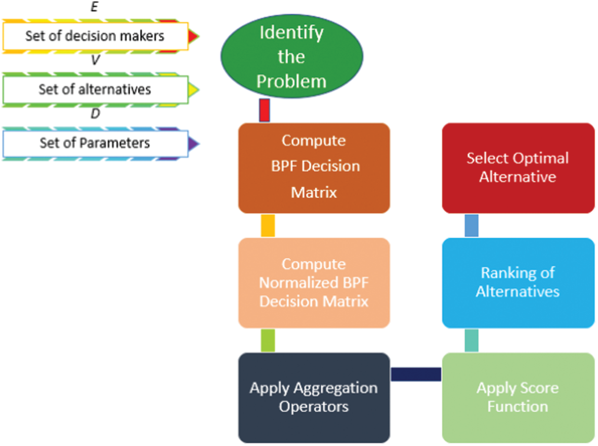
Figure 4: Flow chart of proposed algorithm
We are considering quantitative examples in the selection of mushroom farming alternatives in Pakistan to show the effectiveness of the proposed processes. Filled with taste and an incredible nutritional composition to boot, oyster mushrooms will be a worthy complement to a balanced diet. Here several categories of oyster mushrooms that differ a little in flavor and nutritional benefits. In this paper, we will focus majorly on king oyster mushrooms (KOM) and their nutritional benefits. In all types of mushroom, preparation procedures that we describe can be included. Pleurotus Eryngii (PE) (Fig. 5) is a real term for king oyster mushrooms. They are also known as French horn, royal trumpet, king brown, king trumpet and steppe boletus. The King oyster mushroom is, as its name suggests, the largest of all oyster mushrooms. This is evidently rising in the Middle East and North Africa. It is also extensively grown in Asia, in a variety of countries, as well as in Italy, Australia and the USA. Looking at the health benefits of oyster mushrooms, there are several positive features of this study. Very good sources of riboflavin, iron, niacin, phosphorus, potassium, copper, Protein, vitamin B6, pantothenic acid,folate, magnesium, zinc and manganese from the right source. Mostly limited in cholesterol and saturated fat. Only about 35 per 100 g king oyster mushroom calories. King oyster mushrooms have a good protein source and are the ideal complement to vegetarian or vegan diets. They are not a full source of protein and must ensure that a number of various sources of protein are included in your healthy diet. Alone last year, Americans grew more than two million pounds of exotic mushrooms. Oyster mushrooms, a type of exotic mushrooms, are among the best and fastest growing exotic mushrooms. They could even grow in about six weeks, and they are looking to sell around 6 Dollar a pound wholesale and 12 Dollar a pound retail. They looked incredibly easy to produce, they’re growing quickly, and they can make you decent money–-all the justifications whether you like to oyster mushrooms to grow for financial gain.

Figure 5: King oyster mushroom
KOM is an enormous, important food naturalized to Asia and the rest of Europe. Although hard to find in the wild, it is widely cultivated and famous for its buttery taste and eggplant-like flavor, particularly in some Asian and African cuisines. predominant Chinese medication has for centuries recognized the importance of KOM and other medicative mushrooms.
Here are among the most possibly the best-researched advantages of KOM.
1. Immune System Support
B-glucans in KOM enable them are some of the healthiest meals on the earth to support the immune function toward short-and long-term diseases [51]. Unlike other food products that either activate or inhibit the immune system, the mushrooms balanced the immune cells. Plus, KOM are filled with other antioxidants to help avoid harm caused by free radicals and oxidative stress so that the immune cells can protect itself against aging [52].
2. Reducing of High Blood Pressure
Your body requires nutrients like vitamin D to stabilize your heart rate and blood pressure. Do you think that the majority of people living in colder climates are deficient with vitamin D? One research found that edible mushrooms, such as oysters, reduced blood pressure in rats with chronic or uncertain high blood pressure [53].
3. Regulating Cholesterol Levels
Although mushrooms like KOM have a tasty taste and texture and no cholesterol, they are a fine replacement for meat in several steamed dishes. One study also initiate that in people with diabetes, the intake of oyster mushrooms decreased glucose and cholesterol levels [54].
4. Strong Bones
KOM provide a number of essential ingredients for building better bones. Vitamin D and magnesium in particular. While most persons concentrate on calcium, your body also requires vitamin D and magnesium to absorb and preserve calcium in your bones.
5. Anti-Inflammatory Properties
B-glucans and nutrients in KOM make it a perfect food to reduce inflammation. Some work indicates that, besides B-glucans, some of the anti-inflammatory effects of oysters come from a special and somewhat obscure amino acid called ergothioneine. According to study, ergothioneine reduces “systemic” inflammation around the body, frequently leading to diseases such as dementia and diabetes.
6. Anti-Cancer Properties
B-glucans in mushrooms, such as KOM, serve as powerful antioxidants that can offer some protection from cancer. One research showed that oyster mushrooms have the potential to be involved in some forms of cancer cells.
Various substrates, such as sawdust (SD) and rice straw (RS), have been used to grow KOM. Sun-dried SD, wheat bran and rice husk were combined together. Water was applied to change the water absorption and CaCO3 was blended at a rate of 1% of the mixture. The substrate mixture was packed with airtight plastic polymer bottles. The bottles were sterilized, and after cool back to normal temperature, the sterilized bottles were tested separately. We were using CaCO3, straw, sawdust, corn cob and rice bran to grow King oyster mushrooms. They are combined based on specific ratios, Nguyen et al. [55] take into account each combining formula as an alternative given in Tab. 4.
Table 4: Combining formulas for alternatives
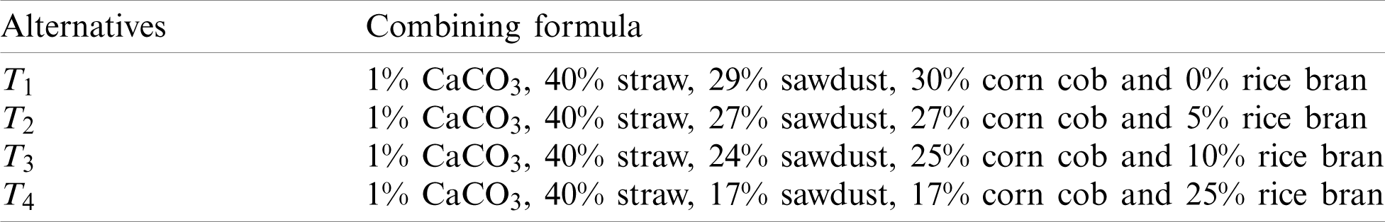
There are four types of alternatives Ti(i = 1, 2, 3, 4), given in Tab. 4. Analysis the effects of rapidly increasing materials on the productivity growth of king oyster mushrooms. We consider C1 = infection rate, C2 = Biological productivity, C3 = diameter of mushroom cap and C4 = diameter of mushroom stalks as attributes. In this example we use BPFNs as input data for ranking the given alternatives under the given attributes. Also, the WV P is (0.3, 0.2, 0.1, 0.4) and standard WV w is (0.2, 0.3, 0.3, 0.2).
Using BPFWG operator
Step 1.
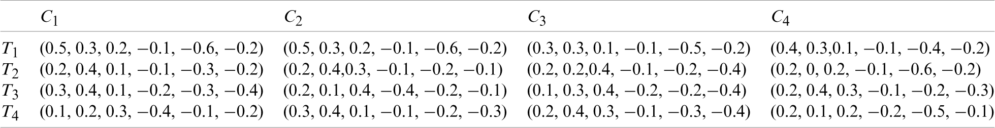
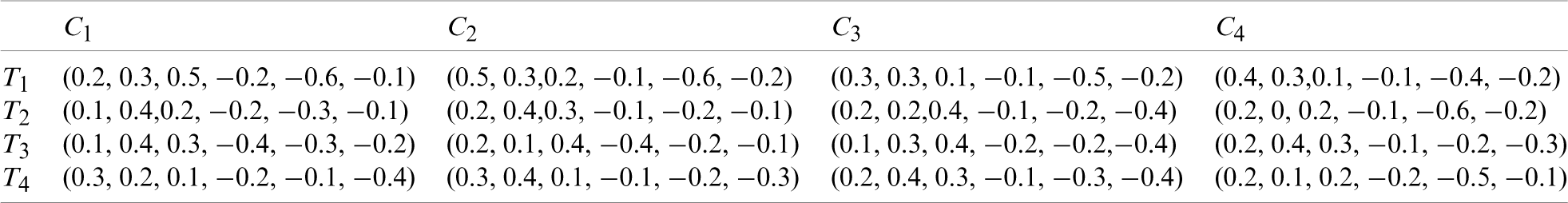
Construct the decision matrix given by the decision maker in Tab. 5 consist on bipolar picture fuzzy information.
Table 5: BPF decision matrix taking by decision maker
Step 2.
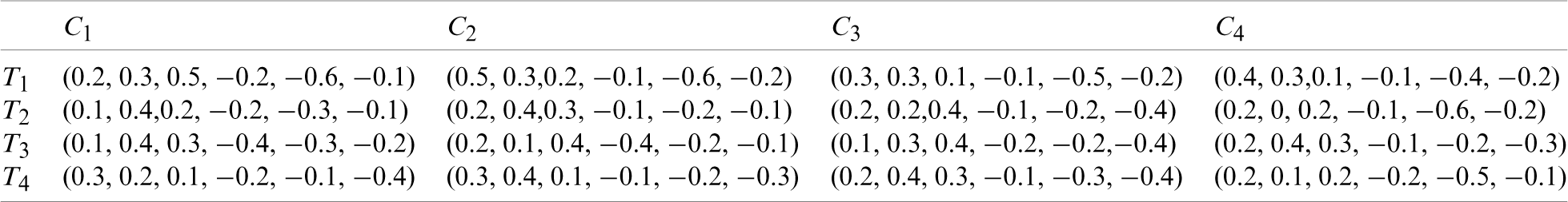
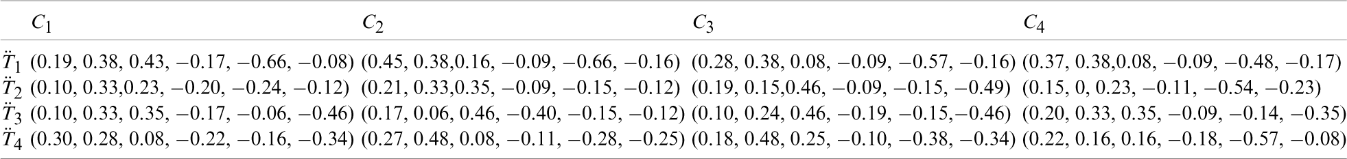
Normalize the decision matrix, because the attribute C1 = price, given in Tab. 6.
Table 6: Normalized BPF decision matrix
Step 3.
Evaluate
Step 4.
Calculate the score functions for all ri.
Step 5.
Rank all the
r2 corresponds to T2, so T2 is the best alternative.
Using BPFOWG operator
Step 1.
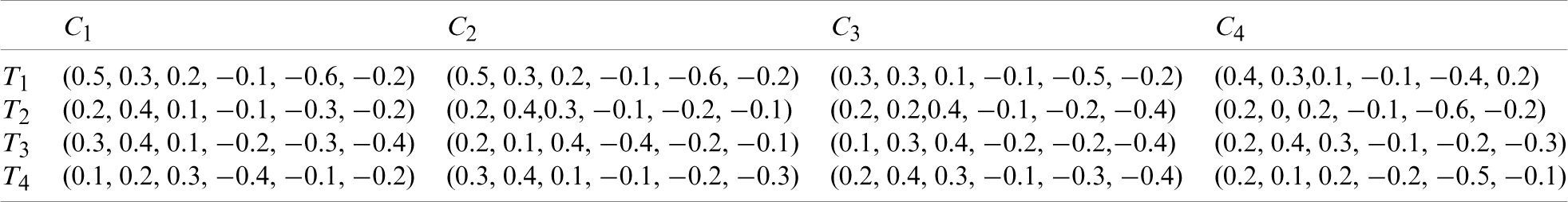
Construct the decision matrix given by decision maker consist on bipolar picture fuzzy information, given in Tab. 7.
Table 7: BPF decision matrix taking by decision maker
Step 2.
Normalize the decision matrix, because the attribute C1 = price, given in Tab. 8.
Table 8: Normalized BPF decision matrix

Step 3.
Evaluate
Step 4.
Calculate the score functions for all ri.
Step 5.
Rank all the
r2 corresponds to T2, so T2 is the best alternative.
Using BPFHG operator
Step 1.
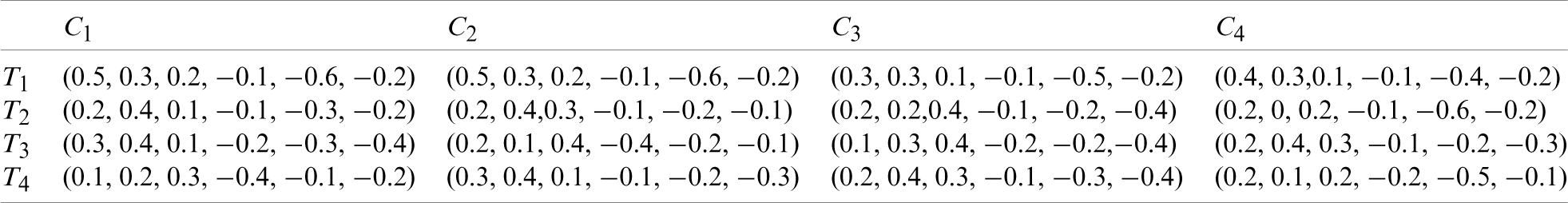
Construct the decision matrix given by decision maker consist on bipolar picture fuzzy information given in Tab. 9.
Table 9: BPF decision matrix taking by decision maker
Step 2.
Normalize the decision matrix, because the attribute C1 = price, given in Tab. 10.
Table 10: Normalized BPF decision matrix
Step 3.
Evaluate
Before evaluating ri we use standard WV to find the
Now,
Step 4.
Calculate the score functions for all ri.
Step 5.
Rank all the
r2 corresponds to T2, so T2 is the best alternative.
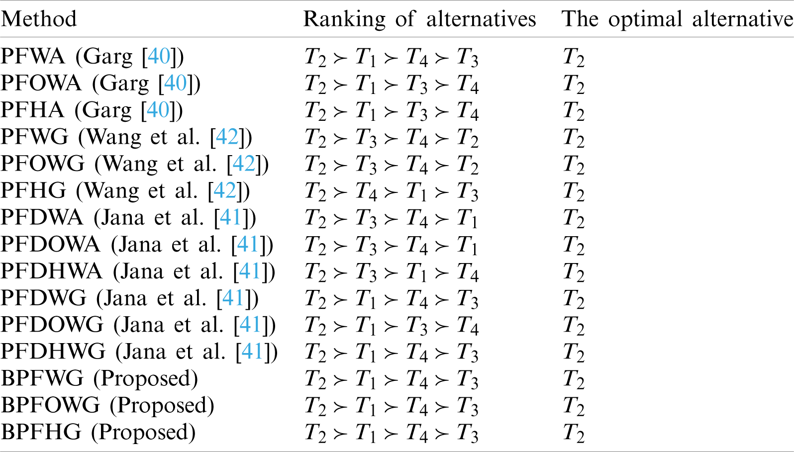
The proposed AOs BPFWG operator, BPFOWG operator and BPFHG operator are compared as shown in Tab. 12 below, which lists the final comparative study ranked among the top four alternatives. The best selection made by any of the proposed operators and current operators, as shown in Tab. 12, validates the consistency and authenticity of the proposed methods.
Table 12: Comparison analysis of the proposed operators and existing operators in the given numerical example
MCDM has been studied to solve complex real-world problems that involve uncertainty, imprecision and ambiguity due to vague and incomplete information. The MCDM techniques practically rely on fuzzy sets and fuzzy models that are considered to address vagueness and uncertainties. The existing fuzzy set theoretic models fail to deal with real life situations when modeling need to assign bipolarity (positive and negative aspects) to each of the degrees of MD (belonging-ness), neutral MD (not-decided), and NMD (refusal). In order to handle such MCDM problems, in this study, we introduced a new extension of fuzzy sets named as BPFS. A BPFS is the hybrid structure of BFS and PFS. The notion of a bipolar picture fuzzy number (BPFN) is superior than existing bipolar fuzzy number and picture fuzzy number. We introduced some algebraic operations and key properties of BPFSs as well as some new distance measures of BPFSs. We presented score function, accuracy function and certainty function for bipolar picture fuzzy information aggregation. Information aggregation plays an important role in the MCDM, and therefore in this study, some new aggregation operators (AOs) named as “bipolar picture fuzzy weighted geometric operator, bipolar picture fuzzy ordered weighted geometric operator, and bipolar picture fuzzy hybrid geometric operator” are developed. Additionally, on the basis of these AOs, a new MCDM approach has been developed for the ranking of objects using BPFNs. The presented scientific method is illustrated by a numerical model to demonstrate its effectiveness and sustainability.
In further research, we can extend proposed aggregation operators to some other MCDM techniques including; TOPSIS, VIKOR, AHP, ELECTRE family and PROMETHEE family. Long term work will pay special attention to Heronian mean, Einstein, Bonferroni mean, Dombi AOs and so on. We keep hoping that our research results will be beneficial for researchers working in the fields of information fusion, pattern recognition, image recognition, machine learning, decision support systems, soft computing and medicine.
Author’s Contributions: The authors contributed to each part of this paper equally. The authors read and approved the final manuscript.
Funding Statement: The authors received no specific funding for this study.
Conflicts of Interest: The authors declare that they have no conflicts of interest to report regarding the present study.
1. Zadeh, L. A. (1965). Fuzzy sets. Information and Control, 8(3), 338–353. DOI 10.1016/S0019-9958(65)90241-X. [Google Scholar] [CrossRef]
2. Atanassov, K. T. (1986). Intuitionistic fuzzy sets. Fuzzy Sets and Systems, 20(1), 87–96. DOI 10.1016/S0165-0114(86)80034-3. [Google Scholar] [CrossRef]
3. Yager, R. R. (2013). Pythagorean fuzzy subsets. 2013 Joint IFSA World Congress and NAFIPS Annual Meeting, pp. 57–61. Edmonton, Canada: IEEE. [Google Scholar]
4. Yager, R. R. (2014). Pythagorean membership grades in multi-criteria decision making. IEEE Transactions on Fuzzy Systems, 22(4), 958–965. [Google Scholar]
5. Yager, R. R., Abbasov, A. M. (2013). Pythagorean membership grades, complex numbers, and decision making. International Journal of Intelligent Systems, 28(5), 436–452. DOI 10.1002/int.21584. [Google Scholar] [CrossRef]
6. Zhang, W. R. (1994). Bipolar fuzzy sets and relations: A computational framework for cognitive modeling and multiagent decision analysis. Proceedings of the First International Joint Conference of the North American Fuzzy Information Processing Society Biannual Conference, pp. 305–309. [Google Scholar]
7. Zhang, W. R. (1998). (Yin Yang) Bipolar fuzzy sets. IEEE International Conference on Fuzzy Systems, vol. 1, pp. 835–840. [Google Scholar]
8. Lee, K. M. (2000). Bipolar-valued fuzzy sets and their basic operations. Proceeding International Conference, pp. 307–317. Bangkok, Thailand. [Google Scholar]
9. Alcantud, J. C. R., Santos-García, G., Peng, X. D., Zhan, J. (2019). Dual extended hesitant fuzzy sets. Symmetry, 11(5), 1–13. DOI 10.3390/sym11050714. [Google Scholar] [CrossRef]
10. Alcantud, J. C. R., Feng, F., Yager, R. R. (2020). An N-soft set approach to rough sets. IEEE Transactions on Fuzzy Systems, 28(11), 2996–3007. DOI 10.1109/TFUZZ.91. [Google Scholar] [CrossRef]
11. Akram, M., Dudek, W. A., Ilyas, F. (2019). Group decision-making based on Pythagorean fuzzy TOPSIS method. International Journal of Intelligent Systems, 34(7), 1455–1475. DOI 10.1002/int.22103. [Google Scholar] [CrossRef]
12. Akram, M., Dudek, W. A., Dar, J. M. (2019). Pythagorean Dombi fuzzy aggregation operators with application in multicriteria decision-making. International Journal of Intelligent Systems, 34(11), 3000–3019. DOI 10.1002/int.22183. [Google Scholar] [CrossRef]
13. Ashraf, S., Abdullah, S., Mahmood, T. (2019). Spherical fuzzy Dombi aggregation operators and their application in group decision making problems. Journal of Ambient Intelligence Humanized Computing, 11(7), 2731–2749. DOI 10.1007/s12652-019-01333-y. [Google Scholar] [CrossRef]
14. Eraslan, S., Karaaslan, F. (2015). A group decision making method based on TOPSIS under fuzzy soft environment. Journal of New Theory, 3, 30–40. [Google Scholar]
15. Feng, F., Zheng, Y., Alcantud, J. C. R., Wang, Q. (2020). Minkowski weighted score functions of intuitionistic fuzzy values. Mathematics, 8(7), 1–30. DOI 10.3390/math8071143. [Google Scholar] [CrossRef]
16. Garg, H. (2019). Neutrality operations-based Pythagorean fuzzy aggregation operators and its applications to multiple attribute group decision-making process. Journal of Ambient Intelligence Humanized Computing, 11(7), 3021–3041. DOI 10.1007/s12652-019-01448-2. [Google Scholar] [CrossRef]
17. Garg, H., Arora, R. (2018). Dual hesitant fuzzy soft aggregation operators and their application in decision-making. Cognitive Computation, 10(5), 769–789. DOI 10.1007/s12559-018-9569-6. [Google Scholar] [CrossRef]
18. Garg, H., Arora, R. (2019). Generalized intuitionistic fuzzy soft power aggregation operator based on t-norm and their application in multicriteria decision-making. International Journal of Intelligent Systems, 34(2), 215–246. DOI 10.1002/int.22048. [Google Scholar] [CrossRef]
19. Jose, S., Kuriaskose, S. (2014). Aggregation operators, score function and accuracy function for multi criteria decision making in intuitionistic fuzzy context. Notes on Intuitionistic Fuzzy Sets, 20(1), 40–44. [Google Scholar]
20. Karaaslan, F. (2015). Neutrosophic soft set with applications in decision making. International Journal of Information Science and Intelligent System, 4(2), 1–20. [Google Scholar]
21. Liu, P., Ali, Z., Mahmood, T., Hassan, N. (2020). Group decision-making using complex q-rung orthopair fuzzy Bonferroni mean. International Journal of Intelligent Systems, 13(1), 822–851. [Google Scholar]
22. Liu, P., Wang, P. (2020). Multiple attribute group decision making method based on intuitionistic fuzzy Einstein interactive operations. International Journal of Fuzzy Systems, 22(3), 790–809. DOI 10.1007/s40815-020-00809-w. [Google Scholar] [CrossRef]
23. Wang, L., Li, N. (2020). Pythagorean fuzzy interaction power Bonferroni mean aggregation operators in multiple attribute decision making. International Journal of Intelligent Systems, 35(1), 150–183. DOI 10.1002/int.22204. [Google Scholar] [CrossRef]
24. Yang, W., Cai, L., Edalatpanah, S. A., Smarandache, F. (2020). Triangular single valued neutrosophic data envelopment analysis: Application to hospital performance measurement. Symmetry, 12(4), 1–14. DOI 10.3390/sym12040588. [Google Scholar] [CrossRef]
25. Smarandache, F. (1999). A unifying field in logics. Neutrosophy: Neutrosophic probability, set and logic. Rehoboth, DE, USA: American Research Press. [Google Scholar]
26. Liu, X., Ju, Y., Yang, S. (2014). Hesitant intuitionistic fuzzy linguistic aggregation operators and their applications to multi-attribute decision making. Journal of Intelligent & Fuzzy Systems, 26(3), 1187–1201. DOI 10.3233/IFS-131083. [Google Scholar] [CrossRef]
27. Naeem, K., Riaz, M., Peng, X. D., Afzal, D. (2019). Pythagorean fuzzy soft MCGDM methods based on TOPSIS, VIKOR and aggregation operators. Journal of Intelligent & Fuzzy Systems, 37(5), 6937–6957. DOI 10.3233/JIFS-190905. [Google Scholar] [CrossRef]
28. Naeem, K., Riaz, M., Afzal, D. (2019). Pythagorean m-polar fuzzy sets and TOPSIS method for the selection of advertisement mode. Journal of Intelligent & Fuzzy Systems, 37(6), 8441–8458. DOI 10.3233/JIFS-191087. [Google Scholar] [CrossRef]
29. Peng, X. D., Yang, Y. (2015). Some results for Pythagorean fuzzy sets. International Journal of Intelligent Systems, 30(11), 1133–1160. DOI 10.1002/int.21738. [Google Scholar] [CrossRef]
30. Peng, X. D., Yuan, H. Y., Yang, Y. (2017). Pythagorean fuzzy information measures and their applications. International Journal of Intelligent Systems, 32(10), 991–1029. DOI 10.1002/int.21880. [Google Scholar] [CrossRef]
31. Peng, X., Selvachandran, G. (2017). Pythagorean fuzzy set: State of the art and future directions. Artificial Intelligence Review, 52(3), 1873–1927. DOI 10.1007/s10462-017-9596-9. [Google Scholar] [CrossRef]
32. Riaz, M., Hashmi, M. R. (2019). Linear Diophantine fuzzy set and its applications towards multi-attribute decision making problems. Journal of Intelligent & Fuzzy Systems, 37(4), 5417–5439. DOI 10.3233/JIFS-190550. [Google Scholar] [CrossRef]
33. Riaz, M., Karaaslan, F., Farid, H. M. A., Hashmi, M. R. (2020). Some q-rung orthopair fuzzy hybrid aggregation operators and TOPSIS method for multi-attribute decision-making. Journal of Intelligent & Fuzzy Systems, 39(1), 1227–1241. DOI 10.3233/JIFS-192114. [Google Scholar] [CrossRef]
34. Riaz, M., Farid, H. M. A., Kalsoom, H., Pamucar, D., Chu, Y. M. et al. (2020). A Robust q-rung orthopair fuzzy Einstein prioritized aggregation operators with application towards MCGDM, Symmetry. Symmetry, 12(6), 1058. DOI 10.3390/sym12061058. [Google Scholar] [CrossRef]
35. Riaz, M., Tehrim, S. T. (2020). Cubic bipolar fuzzy set with application to multi-criteria group decision making using geometric aggregation operators. Soft Computing, 24, 16111–16133. DOI 10.1007/s00500-020-04927-3. [Google Scholar] [CrossRef]
36. Çağman, N., Karataş, S., Enginoglu, S. (2011). Soft topology. Computers and Mathematics with Applications, 62(1), 351–358. DOI 10.1016/j.camwa.2011.05.016. [Google Scholar] [CrossRef]
37. Shabir, M., Naz, M. (2011). On soft topological spaces. Computers and Mathematics with Applications, 61(7), 1786–1799. DOI 10.1016/j.camwa.2011.02.006. [Google Scholar] [CrossRef]
38. Cuong, B. C. (2014). Picture fuzzy sets. Journal of Computer Science and Cybernetics, 30(4), 409–420. [Google Scholar]
39. Cuong, B. C. (2019). Pythagorean picture fuzzy sets, part 1-basic notions. Journal of Computer Science and Cybernetics, 35(4), 293–304. DOI 10.15625/1813-9663/35/4/13898. [Google Scholar] [CrossRef]
40. Garg, H. (2017). Some picture fuzzy aggregation operators and their applications to multicriteria decision-making. Arabian Journal for Science and Engineering, 42(12), 5275–5290. DOI 10.1007/s13369-017-2625-9. [Google Scholar] [CrossRef]
41. Jana, C., Senapati, T., Pal, M., Yager, R. R. (2019). Picture fuzzy Dombi aggregation operators: Application to MADM process. Applied Soft Computing Journal, 74(4), 99–109. DOI 10.1016/j.asoc.2018.10.021. [Google Scholar] [CrossRef]
42. Wang, C., Zhou, X., Tu, H., Tao, S. (2017). Some geometric aggregation operators based on picture fuzzy sets and their application in multiple attribute decision making. Italian Journal of Pure and Applied Mathematics, 37, 477–492. [Google Scholar]
43. Pamucar, D. (2020). Normalized weighted geometric Dombi Bonferoni mean operator with interval grey numbers: Application in multicriteria decision making. Reports in Mechanical Engineering, 1(1), 44–52. DOI 10.31181/rme200101044p. [Google Scholar] [CrossRef]
44. Pamucar, D., Jankovic, A. (2020). The application of the hybrid interval rough weighted Power-Heronian operator in multi-criteria decision making. Operational Research in Engineering Sciences: Theory and Applications, 3(2), 54–73. DOI 10.31181/oresta2003049p. [Google Scholar] [CrossRef]
45. Ramakrishnan, K. R., Chakraborty, S. (2020). A cloud TOPSIS model for green supplier selection, Facta Universitatis series. Mechanical Engineering, 18(3), 375–397. [Google Scholar]
46. Riaz, M., Pamucar, D., Athar Farid, H. M., Hashmi, M. R. (2020). q-Rung orthopair fuzzy prioritized aggregation operators and their application towards green supplier chain management. Symmetry, 12(6), 976. DOI 10.3390/sym12060976. [Google Scholar] [CrossRef]
47. Riaz, M., Razzaq, A., Kalsoom, H., Pamucar, D., Athar Farid, H. M. et al. (2020). q-Rung orthopair fuzzy geometric aggregation operators based on generalized and group-generalized parameters with application to water loss management. Symmetry, 12(8), 1236. DOI 10.3390/sym12081236. [Google Scholar] [CrossRef]
48. Si, A., Das, S., Kar, S. (2019). An approach to rank picture fuzzy numbers for decision making problems. Decision Making: Applications in Management and Engineering, 2(2), 54–64. DOI 10.31181/dmame1902049s. [Google Scholar] [CrossRef]
49. Sinani, F., Erceg, Z., Vasiljevic, M. (2020). An evaluation of a third-party logistics provider: The application of the rough Dombi-Hamy mean operator. Decision Making: Applications in Management and Engineering, 3(1), 92–107. [Google Scholar]
50. Delia, I., Ali, M., Smarandache, F. (2015). Bipolar neutrosophic sets and their application based on multi-criteria decision-making problems. Proceedings of the 2015 International Conference on Advanced Mechatronic Systems, Beijing, China. [Google Scholar]
51. Abdullah, N., Abdulghani, R., Ismail, S. M., Abidin, H. Z. (2017). Immune-stimulatory potential of hot water extracts of selected edible mushrooms. Food and Agricultural Immunology, 28(3), 374–387. DOI 10.1080/09540105.2017.1293011. [Google Scholar] [CrossRef]
52. Tanaka, A., Nishimura, M., Sato, Y., Nishihira, J. (2016). Enhancement of the TH1-phenotype immune system by the intake of oyster mushroom (Tamogitake) extract in a double-blind, placebo-controlled study. Journal of Traditional and Complimentary Medicine, 6(4), 42. [Google Scholar]
53. Alam, N., Yoon, K. N., Lee, J. S., Cho, H. J., Shim, M. J. et al. (2011). Dietary effect of pleurotus eryngii on biochemical function and histology in hypercholesterolemic rats. Saudi Journal of Biological Sciences, 18(4), 403–409. DOI 10.1016/j.sjbs.2011.07.001. [Google Scholar] [CrossRef]
54. Cho, J. H., Kim, D. W., Kim, S., Kim, S. J. (2017). In vitro antioxidant and in vivo hypolipidemic effects of the king oyster culinary-medicina mushroom, pleurotus eryngi var. ferulae DDl01 (agaricomycetesin rats with high-fat diet-induced fatty liver and hyperlipidemia. International Journal of Medicinal Mushrooms, 19(2), 107–119. DOI 10.1615/IntJMedMushrooms.v19.i2.20. [Google Scholar] [CrossRef]
55. Nguyen, T. B. T., Ngo, X. N., Nguyen, T. T., Tran D. A. (2016). Evaluating the growth and yield of king oyster mushroom (Pleurotus eryngii (DC.:Fr.) Quel) on different substrates. Vietnam Journal of Agricultural Sciences, 14(5), 816–823. [Google Scholar]
 | This work is licensed under a Creative Commons Attribution 4.0 International License, which permits unrestricted use, distribution, and reproduction in any medium, provided the original work is properly cited. |