Computer Modeling in Engineering & Sciences

DOI: 10.32604/cmes.2021.012386

ARTICLE

Analysis of Turbulent Flow on Tidal Stream Turbine by RANS and BEM

Younes Noorollahi1,2,*, Mohammad-Javad Ziabakhsh Ganji1, Mohammadmahdi Rezaei1,2 and Mojtaba Tahani3

1Department of Renewable Energy and Environmental Engineering, Faculty of New Sciences and Technologies, University of Tehran, Tehran, 1439957131, Iran
2Energy Modelling and Sustainable Energy System (METSAP) Research Laboratory, Faculty of New Sciences and Technologies, University of Tehran, Tehran, 1439957131, Iran
3Department of Aerospace Engineering, Faculty of New Sciences and Technologies, University of Tehran, Tehran, 1439957131, Iran
*Corresponding Author: Younes Noorollahi. Email: noorollahi@ut.ac.ir
Received: 29 June 2020; Accepted: 27 January 2021

Nomenclature

1  Introduction

According to the recorded statistics during the past 30 years, global energy demand has increased considerably. In 1990, global final energy consumption was equal to 6.26 billion tonnes of crude oil equivalent. In 2017, it was increased to 9.72 billion tonnes of crude oil equivalent. This trend showed an average annular increase of 1.3% and a total increase of 55.1% in energy consumption. Global energy consumption is currently around ten billion tonnes of crude oil equivalent per year, while it is predicted that it increases to 19.328 billion tonnes by 2040 [1]. Thus, the vital question is whether or not fossil energy resources can meet the world’s energy needs for future evolution and development. Based on the following reasons, the answer to this question is no, and new energy resources should be substituted with the current ones:

—   Environmentally, Fossil fuels release toxic air pollutants long before they are burned. Indeed, millions of people are endangered daily to toxic air pollution from active oil and gas reservoirs and processing facilities. Also, fossil fuels produce massive amounts of carbon dioxide when burned. Carbon emissions ambush heat in the atmosphere and lead to climate change.

—   Technically, all fossil fuels energy carries are exhaustible resources and will sooner or later run out. Also, the use of their unconventional resources is not yet economical and cannot be justified.

Among the renewable energies, hydropower is considered an essential energy resource obtained in oceans [2]. This kind of energy is called ocean energy, ocean power, marine energy, or marine power. The oceans and seas have a wide range of potential in renewable energies using their waves, tides, the temperature gradient between deep cold water and shallow warm water, and salinity gradient in estuaries. Combination of the earth’s rotational effect, the gravity of the moon, and the sun on the earth cause tides on water. Accordingly, many energy generation systems are designed to extract energy from this natural phenomenon [3].

Benhamadouche et al. [4] have estimated the cross-flow in a staggered tube bundle in both 2D and 3D areas with the FVM approach. They have tried LES and RSTM methods, but in the end, they have resulted in that there was no advantage of the RSTM over the LES. Molland et al. [5] have collected experimental measurements for three years between 2005 and 2007. Their results presented the average power and thrust in various depths and blade and hub angles in both cavitation tunnel and spare tank. Battern et al. [6] have reported various simulation tools based on the blade element momentum method. They conducted a study based on the generalization of wind turbines and ship’s propellers to horizontal axis tidal turbines on a scale of 1/20th. Jimenez et al. [7] have utilized the Large–Eddy Simulation (LES) to simulate the wake behaviour in a drag-based simplified turbine model. Ferrer et al. [8] had performed a comparison between BEM and CFD (RANS) models for simulating the wind turbines. In 2010, Calaf et al. [9] used the LES model to simulate a wind turbine farm modelled using a classical drag-disk concept. In 2011, Lu et al. [10] integrated a three-dimensional large-eddy simulation with an actuator line technique. Turnock et al. [11] have developed an improved method to merge an inner domain solution of BEM theory with an outer domain solution of RANS equations for assessing the performance of tidal turbines. The angular momentum and turbulence intensity source have been used to model the near wake evolution besides the usually applied axial momentum source terms. This study shows that power production is sensitive to lateral and longitudinal separation relative to the mean tidal direction separation. A small lateral and significant longitudinal separation is the most effective combination [11]. In 2013, Churchfield et al. [12] utilized the LES model to study wake propagation and power production in various tidal-current turbines using rotating actuator lines. Malki et al. [13] have used the BEM in conjunction with the RANS k–ϵ model to evaluate the performance of a laboratory scaled turbine. Studies were made around the turbulent bending moments that caused by an ocean current turbine placed in a tidal channel in tidal current boundary layers with the LES approach from 2015 until 2017 [14,15]. Researches are also underway to simulate the turbulent flow of large-Eddies around tidal turbines. Turbines affected by wake shadowing operate in more arduous flow circumstances, such as higher turbulence levels or lower conflict velocity [16]. These lead to reduced performance and more massive fatigue loading in tidal turbines. To overcome those kinds of problems, a group of 3 scientists has analyzed array spacing on tidal stream turbine farms [17]. Song et al. [18] have offered a new layout for a blade with salinity corrosion resistance and mechanical fatigue resistance, based on numerical simulation and fatigue tests. The one-way fluid-structure interaction (FSI) representation for an ocean current turbine blade has been set and calculated by a CFD and FEM solver. The project results provide supervision for optimizing the structural design of ocean current turbine blades [18]. In another project by Song et al. [19], three main factors that affect the hydrodynamic performance, including the flow shear rate, the yaw angle, and arrangement rule in the array, have been considered to get closer to the actual working environment of a tidal flow turbine. It has been found that the various shear rate of flow will result in power and axis thrust inconsiderably amplitude comparing with the uniform flow, and a diffuser turbine will further expand this effect compared with a bare turbine [19].

Using these kinds of numerical methods (BEM, RANS, LES, ALM, etc.) is not costly and can be useful for the initial design and analysis of the data. However, due to the inherent weakness in solving the transient features of flow such as blade-tip vortex, a transition from laminar to turbulent flow, flow separation, and even creation of fluctuations downstream, they cannot be used for a comprehensive analysis of turbine performance [20,21]. On the other hand, McSherry et al. [22] have numerically simulated the same laboratory scaled turbine as the works are done by Molland et al. [5] by considering the whole blade geometry. They present numerical simulation results using the blade element momentum method for a three-bladed horizontal axis tidal turbine. It was modelled experimentally by Bahaj et al. [22,23] to validate the thrust coefficients and the power output. The results for a pitch angle of 20 at the blade tip speed ratios of 4 to 10 are compared with experimental results [22,23].

In this study, the rotating geometry simulation has been used for modelling. The current work’s main innovation is utilizing a frozen rotor method, a time-averaging scheme, to connect the rotating volume boundaries and the stationary volume. Here, the computational domain is divided into stationary and rotating regions. The unsteady flow is divided into steady and time-averaged flows. This method employs the relative motion between different zones and transfers the calculated values between these zones. In the unsteady methods, the mixing plane produces the average values through the rotor and stator gap. In contrast, in the frozen rotor method, the obtained values are transferred between the intermediate plane’s two sides. Therefore, to observe the wakes downstream, it is recommended to use the frozen rotor method.

2  Designed Structure Specification

The purpose of this study is to numerically simulate a laboratory scaled horizontal axis tidal turbine (including three blades, hub, and base) using the k–ωSST turbulent model [24]. The tidal turbine blade consists of a few NACA 6-series profiles with various chords, thicknesses, and pitch angles at various radiuses [25]. This turbine’s experimental model has been created in the water tunnel laboratory at the University of Southampton by Batten et al. [6]. According to the parameters presented in Tab. 1, Bahaj et al. [23] have built the blades in the laboratory scaled at various radiuses (Fig. 1). Accordingly, the NACA 63-8xx has been used as the airfoil profile.

Table 1: The design parameters of the turbine blade

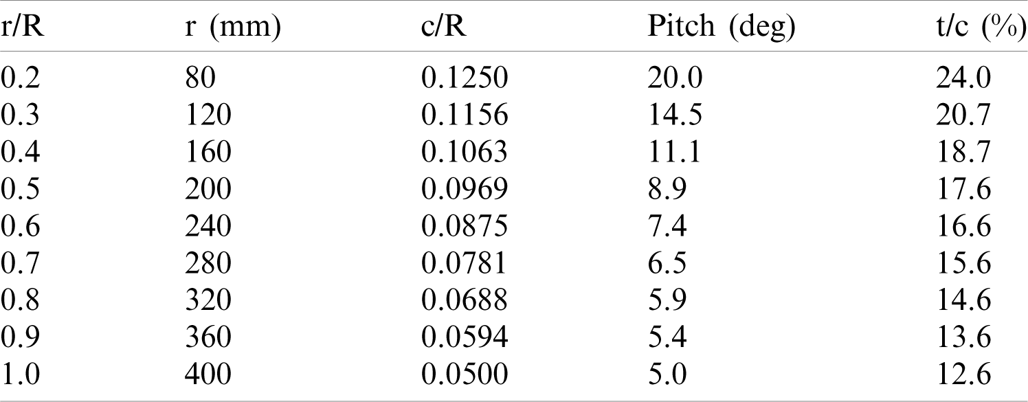
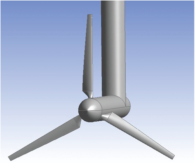
Figure 1: Schematic of the designed turbine

2.1 Dimensions and Accuracy of the Grid

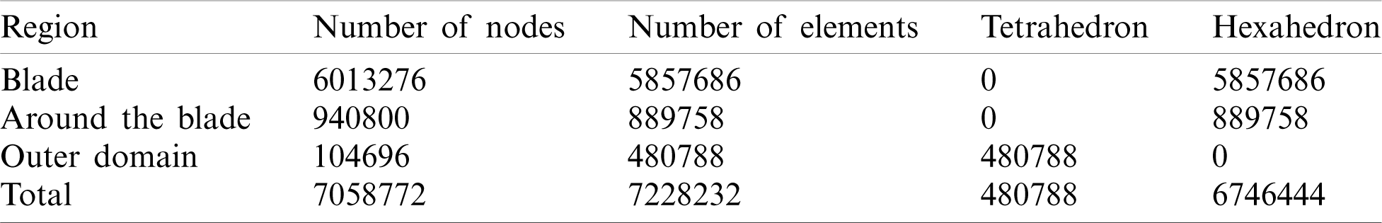
The horizontal axis tidal turbine geometry has been divided into rotating and stationary volumes to generate the grids. The rotating part consisted of a cylinder, and the turbine blades rotate with a given blade-tip speed. This part has been divided into a hexahedron part and an outer part which have meshed structurally to achieve a reasonable accuracy and decrease the convergence time. Fig. 2 demonstrates the rotating volume grid. The rotating part is repeatable (symmetric) in every 120 degrees. Thus, it is appropriate to generate a grid only for one-third of the domain. The stationary volume is created separately using the control matching and interface. This volume has meshed using tetrahedron elements so that the size of its elements was twice the blade chord. Tab. 2 represents the number and type of elements used in the computational domain consisted of three blades.

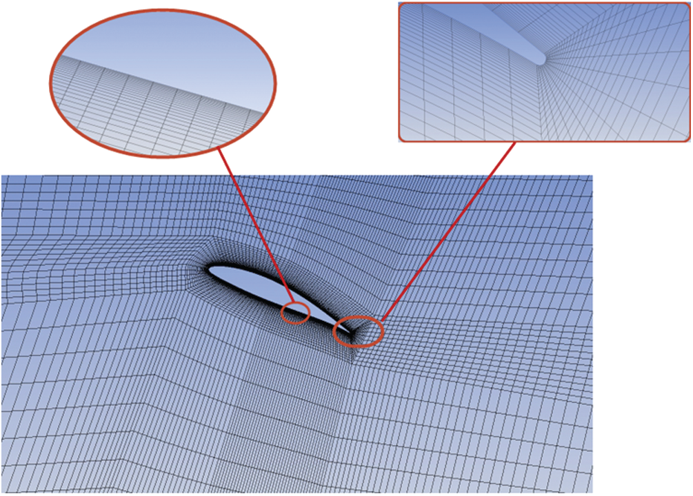
Figure 2: The structural mesh for the plate

Table 2: Types of elements used in the computational domain

3  Research Methodology

3.1 Numerical RANS Method

Menter’s SST turbulent model was applied to combine the k–ω model, which has a proper function in the vicinity of the walls, and k–ω model, which has an appropriate function in regions far from the walls [24]. In the k–ω model, the turbulence frequency (ω) calculates the turbulent viscosity instead of the loss rate (ϵ). Unlike the k–ϵ model (Eq. (1)), a high Reynolds model, the k–ω model (Eq. (2)) also considers the effects of low Reynolds numbers, compressibility, and shear flow separation.

μt=ρcμκ2εPK=μt(∂ui¯∂xj+∂uj¯∂xi)∂ui¯∂xj-23(ρκ+μt∂ul∂xl)∂u¯k∂xk=μtφ2 (1)

μt=ρcμκ2ωPκ=μt(∂ui¯∂xj+∂uj¯∂xi)∂ui¯∂xj-23(ρκ+μt∂ul∂xl)∂uκ∂xκ=μtφ1 (2)

The SST model can utilize the k–ω model for low Reynolds regions and using the k–ε model in high Reynolds regions [26]. Accordingly, to combine these two models, it is necessary to formulate the k–ω model in the form of the k–ω one. This model firstly modifies the energy production term in the kinetic energy transfer equation. So, Eq. (2) in the k–ω turbulence model is replaced by the following expression in the SST model:

Pκ= min(μtφ,Clmtε)(3)

The Clmt value frequently is considered to be 1015. Eq. (3) is the same as Eq. (2), in which the SST model selects the appropriate value according to the region in question. Besides, in the SST model, a new term for losses in the equation appears, which is in the form of Eq. (4):

(1-F1)2ρσω2ω[∂k∂x∂ω∂x+∂k∂y∂ω∂y+∂k∂z∂ω∂z](4)

In Eq. (4), F1 is the mixing function near the wall surface, zero away from the wall. Using the F1 value, the SST model automatically uses the k–ω model near the wall and the k–ϵ model in the far wall. All coefficients in the SST model are calculated as a function of F1, where ϕ is the principal coefficient of the SST model, and ϕ1 is calculated from the k–ω model and ϕ2 from the k–ϵ model.

φ=F1φ1+(1-F1)φ2(5)

Therefore, the SST two-equation turbulent model was used in the ANSYS-CFX software for the numerical simulations.

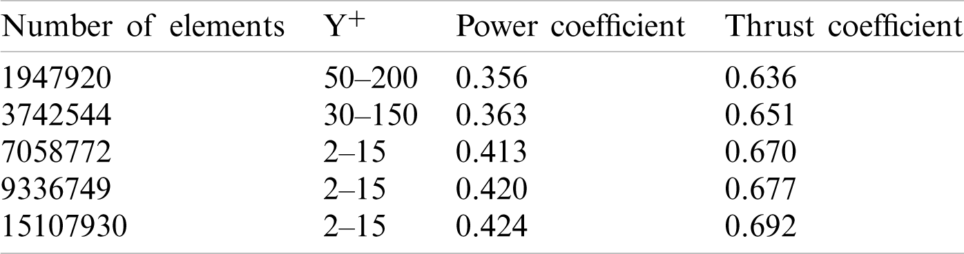
3.1.1 Study of the Grid Independency

The sensitivity of the solution to the grid should be investigated to validate the numerical results. Therefore, the power and thrust coefficients at a speed ratio of 5 have been chosen to evaluate various mesh sizes’ effect on the numerical results. Tab. 3 shows the variations of power and thrust coefficients and Y+ (the quality of boundary layer grid) for different grid numbers. According to Tab. 3, the variation in the grids’ mentioned parameters with higher than 7058772 elements is negligible. Thus, a grid with 7058772 elements has been used for numerical simulations.

Table 3: The sensitivity of the numerical solution to grid number

3.2 Blade Element Momentum (BEM)

The blade element momentum theory is based on a combination of momentum and blade element methods. The momentum theory can be used to calculate axial and rotational flow coefficients for a finite number of rotor blades considering the tip-loss factor. The blade element theory can model the drag and torque by dividing the rotor blade into non-interacting sections [8].

A combination of these theories means that at the radius of each blade, the axial loadings on the rotor, (dCp)/d(r/R) and the power loadings (dCp)/d(r/R), have determined using matching the fluid momentum variations and the blade forces based on the drag and lift coefficients (CD and CL) at various attack angles. The limit for the number of rotor blades was determined using Goldstein’s tip-loss approximation. Combining the blade’s loadings, the torque, drag, and power coefficients on the rotor are be obtained. Based on the blade element momentum theory, the numerical codes were written [27]. Fig. 3 shows the flowchart of the numerical model, which indicates how the numerical code can be used for both types of loadings as well as investigating the cavitation inside the domain. Also, the direction of forces and blade angles are presented in Fig. 4. Based on Eq. (6), The turbine power (B) is equal to the multiplication of the applied torque on the blade (T) and the angular velocity of the blade (ω). Also, as mentioned in Eq. (7), the blade-tip speed ratio, known as TSR, is equal to the blade tip’s linear velocity (Rω) divided by the free stream velocity (V).

B=T×ω (6)

TSR=λ=Rω/V (7)

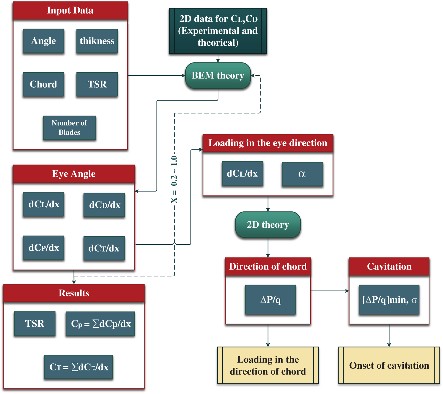
Figure 3: Flowchart of the numerical model

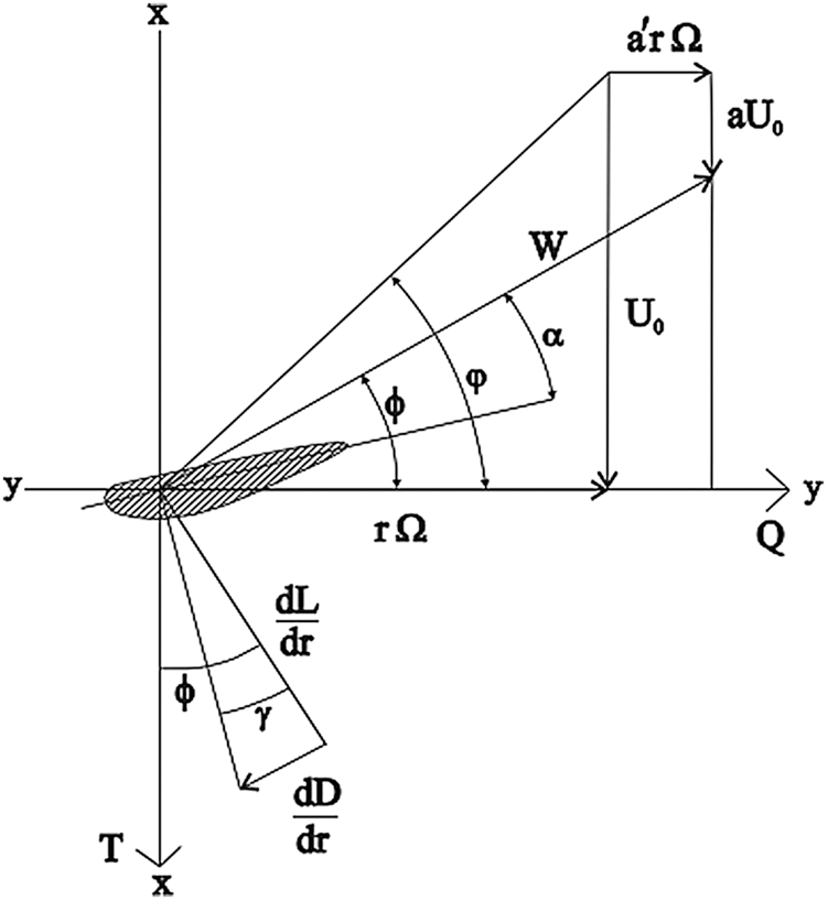
Figure 4: Forces on the ocean stream turbine blade [28]

4  Boundary Conditions and Fluid Properties

At the inlet of the domain for analyzing the fluid flow around the horizontal axis tidal turbine, a velocity with a linear profile was applied, which was calculated based on the laboratory system. The fluid used for the simulation was water at 25∘C with a density of 997 kg/m3 and the kinematic viscosity of 10-6m2/s. According to the experimental data, the turbulent intensity has set equal to 5%, and the open channel boundary condition with relative pressure of zero has also been used at the outlet. Also, the symmetry boundary condition has been applied to the side and top walls of the domain.

The frozen rotor method, a time-averaging method, has implemented simulations to connect the domain’s rotating and stationary parts. Here, the computational domain is divided into stationary and rotating volumes, and the unsteady flow is divided into a steady flow and a time-averaged flow. A no-slip condition with a relative roughness of 100 μm was applied on the stationary and moving walls. As shown in Fig. 5, the computational domain has an upstream length of 4D (D is equal to the blade chord), downstream length of 10D, a width of 5D, and depth of 2.5D.

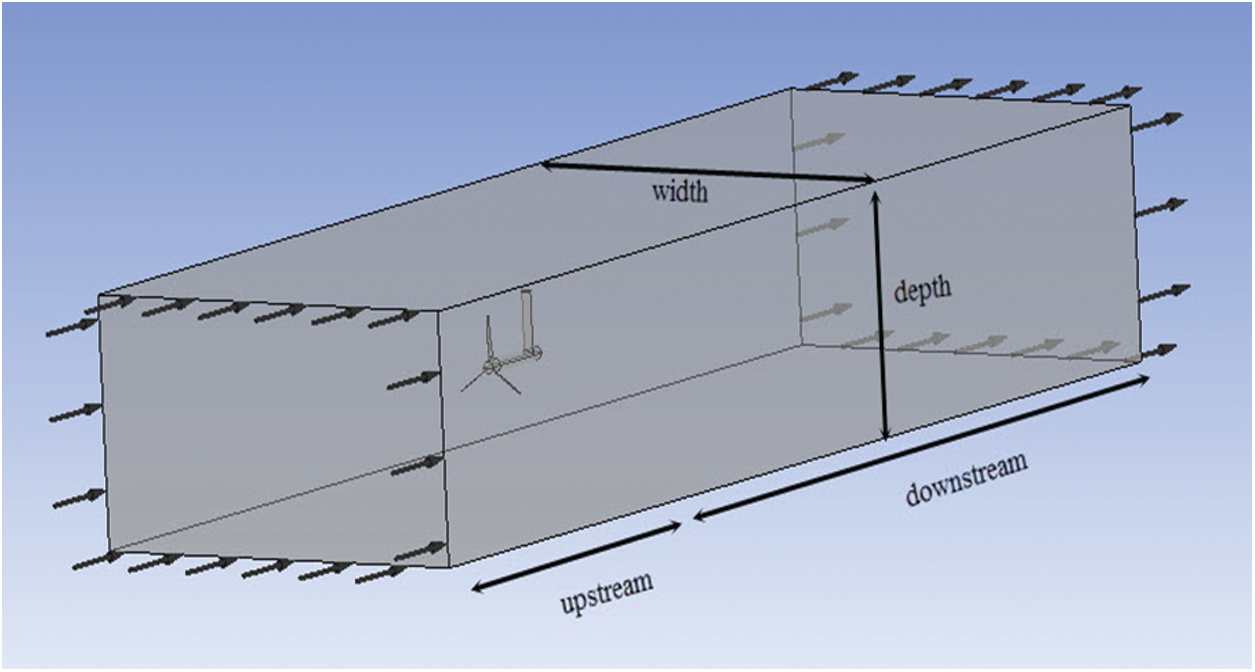
Figure 5: The computational domain for the considered tidal turbine

5  Result and Discussion

The pressure variation and velocity are two critical parameters in fluid dynamic analysis. The calculation of these two parameters leads to the determination of other ones. Fig. 6 shows the pressure variations around the turbine from the side and top perspectives. As was expected, when the fluid meets the turbine, the pressure decreases, and due to the first stage of pressure drop and the rotor’s large sweep volume, the maximum variation of pressure occurs on the turbine blade.

The negative pressure is caused by the flow circulation, i.e., backward flow, or the wakes formed in the flow field [29]. The significant variation of pressure on the turbine blades represents the high value of thrust force on the blade. This is one of the forces which are considered during the turbine blade design. Then, the pressure drops decreases while the fluid flows from the turbine base to the tower. The wake effect and pressure drop will continue until 7D downstream. This effect is critical in analyzing a tidal turbine farm. Since the flow is turbulent and the blade rotates in a specific direction, the pressure drop is higher at this part of the blade. Fig. 7 shows the velocity contour. In this figure, the tip and tower effect on the instantaneous velocity can be seen in the middle of the plane and at the inlet velocity of 1.73 m/s. There is a decrease in fluid rate in front of the turbine due to the wave created in the fluid after impacting the turbine wall. There will be a wake behind the turbine tower based on the outcomes shown in Fig. 7.

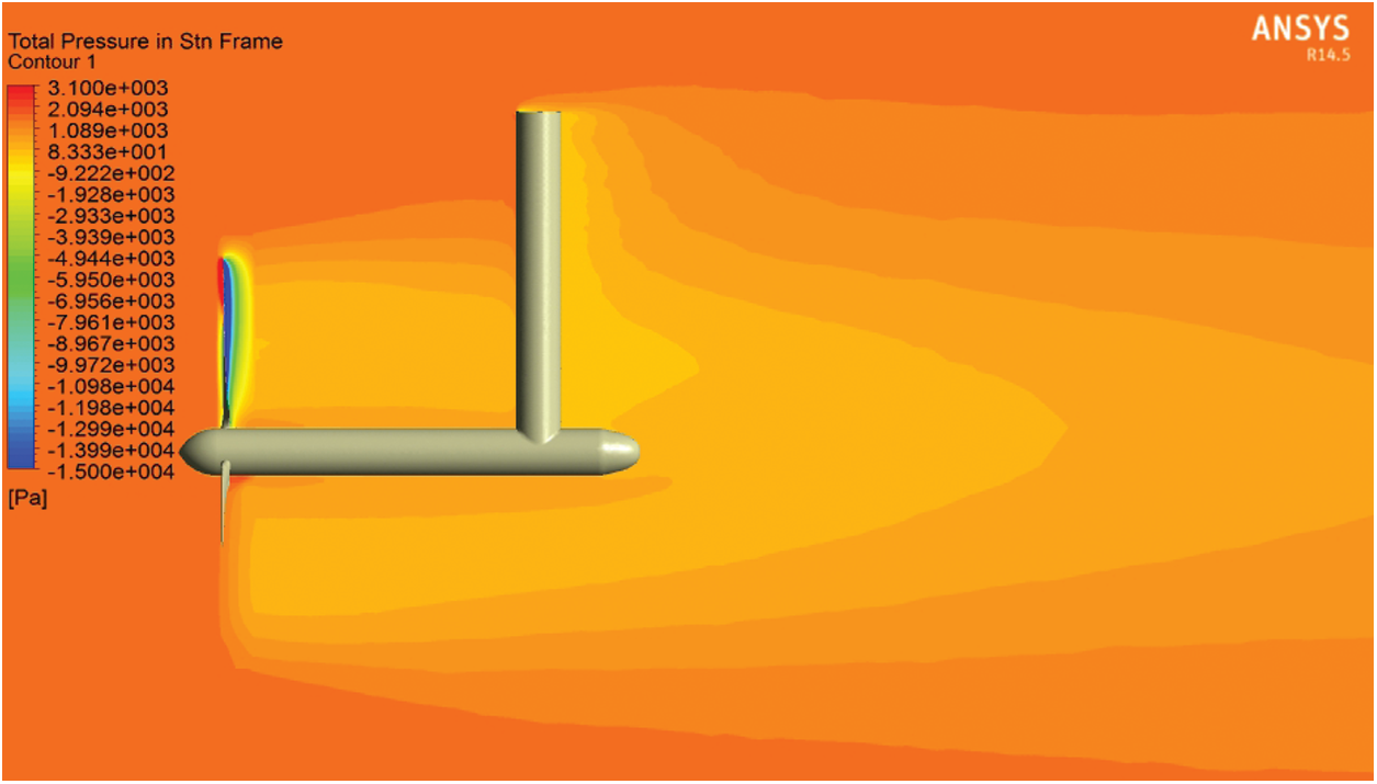
Figure 6: The pressure gradient contour at the inlet velocity of 1.73 m/s

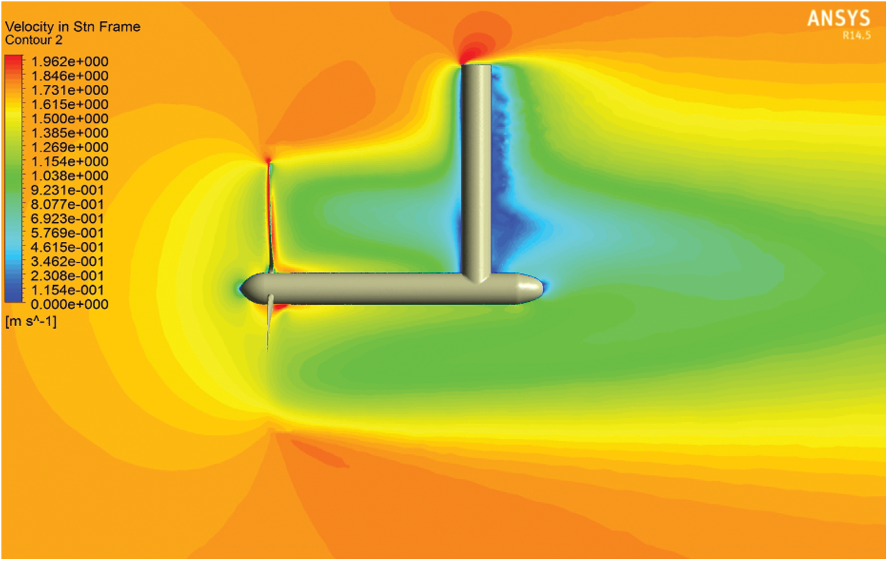
Figure 7: The contour of velocity magnitude at the inlet velocity of 1.73 m/s

The pressure gradient on the blade surface is shown in Fig. 8 over the front perspective. These results can be used in turbine structural analysis. In the computational fluid dynamics and solution methods such as k–ωSST, in which the governing equations are solved in the vicinity of walls, the boundary layer grids are vital [30]. The Y+ parameter has used to determine the grid quality inside the boundary layer. The Y+ value has set to the range of 2–30 for this study. Fig. 9 shows the Y+ contour on the blade surface, which has the most sensitivity to the grid quality. According to Fig. 9, the Y+ value of more than 90% of the blade surface is less than 8. The vector plot of the velocity field on the middle plane is presented in Fig. 10. This figure also shows the direction of rotation and the linear velocity variations with increasing the local radius.

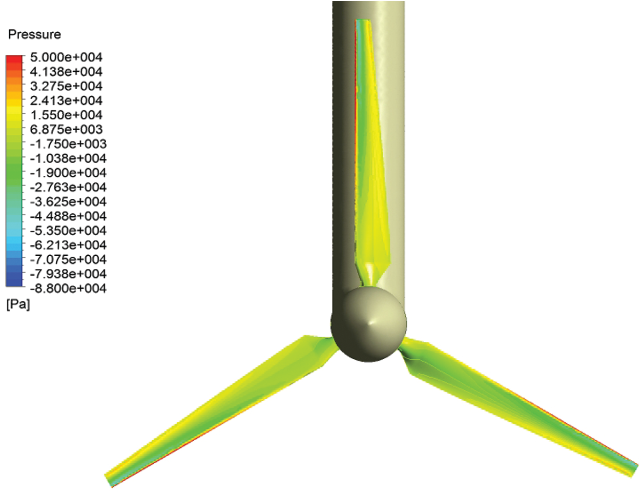
Figure 8: The pressure variation on the blade surface

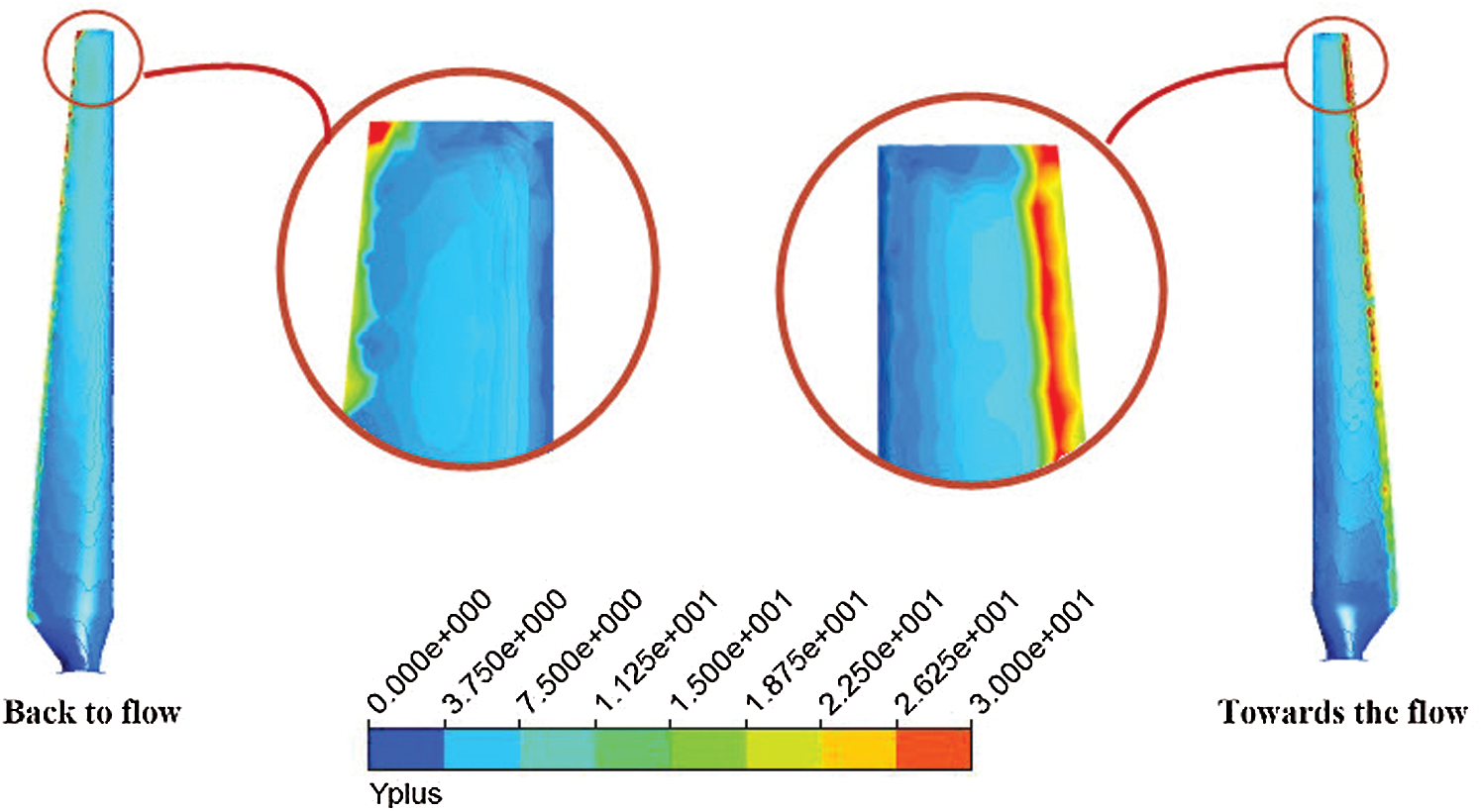
Figure 9: The contour of Y+ on the blade surface

The simulated outcomes have been compared with experimental ones to validate the obtained results. In horizontal axis tidal turbines, the power and thrust coefficients are essential in both experimental and numerical simulations. Fig. 11 shows the CFD results, BEM, and the experimental methods for variation of power coefficient Cp vs. the speed ratio. Accordingly, the maximum deviation of CFD results from the experimental outcomes at the blade-tip ratios between 4 to 10 is less than 8%. In the blade element momentum (BEM) method, the maximum deviation of obtained results from the experimental ones at blade-tip ratios between 4 and 8 is less than 5%. The blade-tip ratios higher than 8 are around 10%. The increase in tip ratio at a fixed free stream velocity leads to an increase in the angular momentum. Since the increase in angular velocity is more significant than the torque variations to a particular value of speed ratio, the turbine’s received power will increase, too. However, since the increased relative velocity between the angular velocity and the linear velocity of fluid causes the flow separation on the blade and decreases the torque, the turbine’s received power will decrease after a particular speed ratio value.

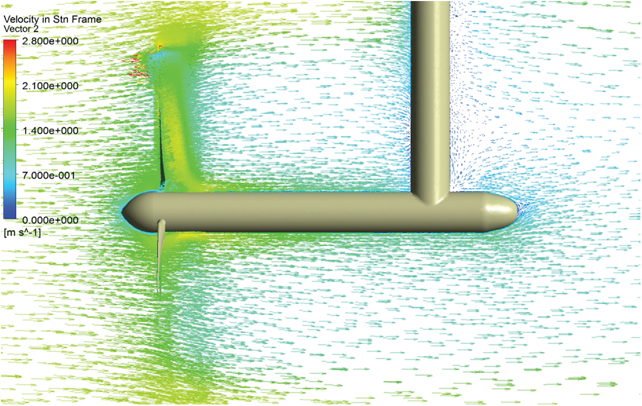
Figure 10: Vector plot of velocity from the side perspective

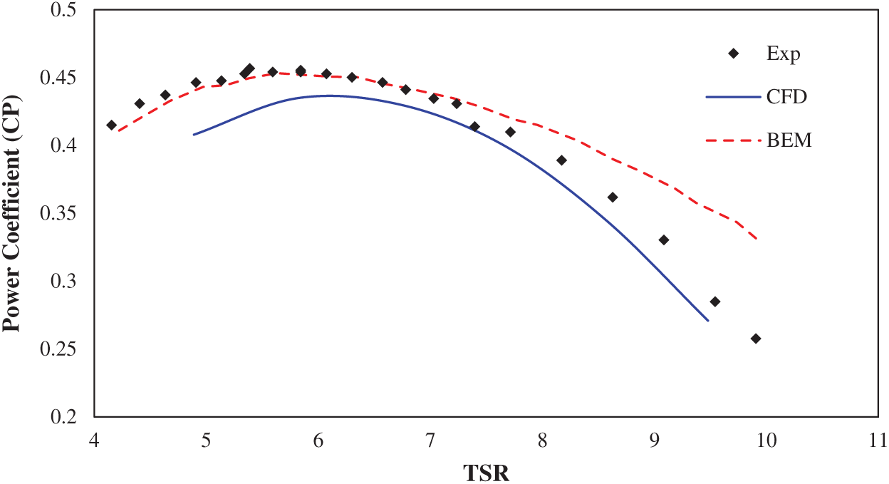
Figure 11: Variation of the power coefficient relative to the speed ratio

At a fixed free stream velocity, the turbine encounters different speed ratios related to the power generator control and gearbox systems used in the feedback part and the lack of rotor ability to rotate in proportion with the instantaneous fluid velocity. Usually, it is fixed at the constant value of ω. The best value for ω is the one that leads to the highest output power. According to the previous research, the variations of power and thrust coefficients are proportional to the blade-tip speed ratio in horizontal axis wind and tidal turbines. Therefore, the variations of power and thrust coefficients are always plotted relative to the speed ratio. This ratio is a dimensionless number for this kind of turbine. In other words, to compare the turbines, the speed ratios should be the same, i.e., the ratio of power and thrust coefficients blade-tip speed ratio should be constant. Fig. 12 presents the comparison between the thrust coefficient variations obtained from CFD and BEM methods as a speed ratio function.

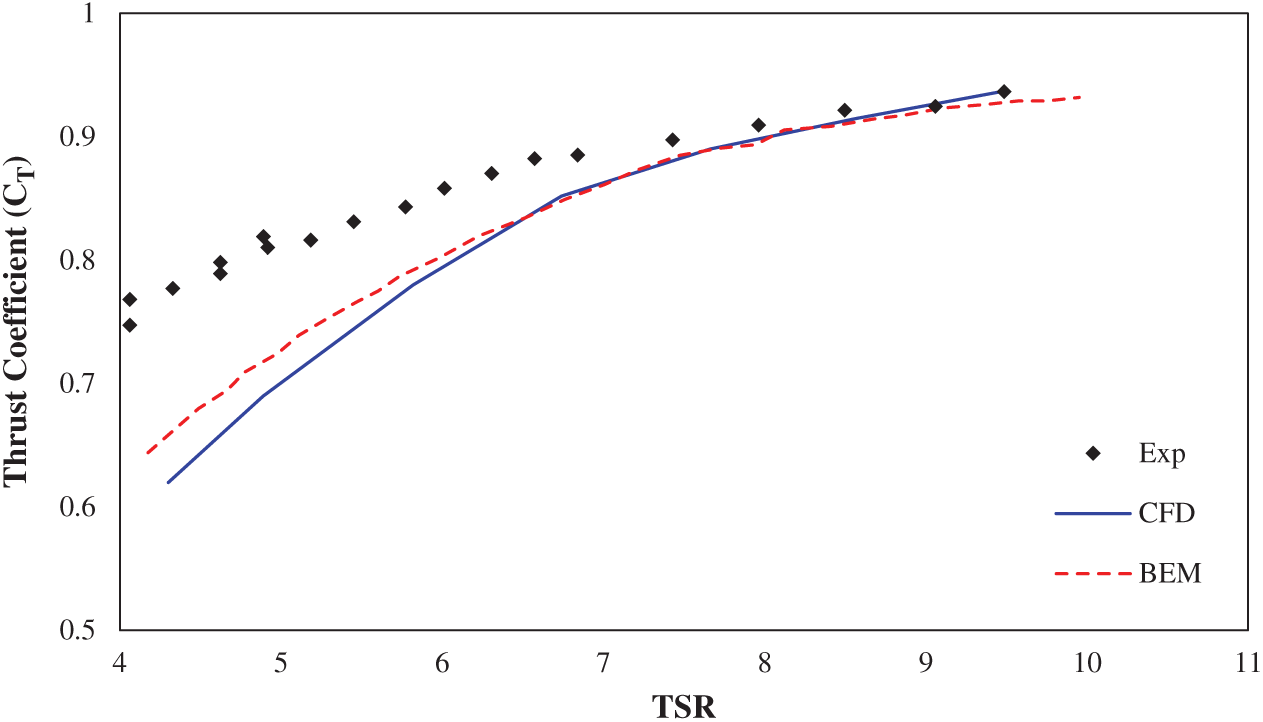
Figure 12: Variation of the thrust coefficient relative to the speed ratio

The thrust force, i.e., the drag force on the turbine, is enhanced by increasing the tip ratio to 7. The thrust force will not grow in tip ratios higher than seven due to the rotor’s flow blockage. The variations of static power coefficient at different sections of the turbine blade at the speed ratio of 7 are shown in Figs. 13 and 14. As shown in Figs. 13 and 14, the results show that the power coefficient’s absolute value in the turbine’s initial parts is incremental. For positive values, Cp decreases in the median ratios (up to 0.5), and then, as the X/C increase, all the radial ratios will increase convergently. The Cp’s negative values follow the same procedure as the positive coefficients, with the difference that their convergence will increase significantly after a 0.5 X/Cratio.

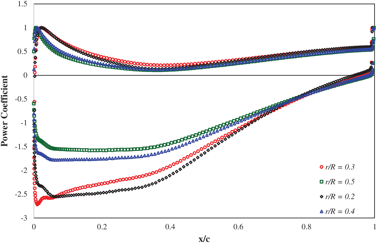
Figure 13: Variation of power coefficient in various blade sections at the speed ratio of 7

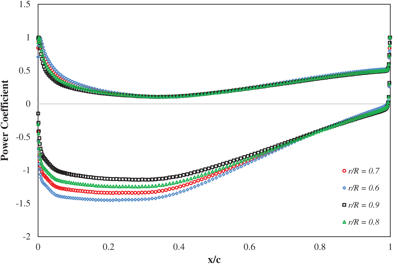
Figure 14: Variation of power coefficient at various blade sections at the speed ratio of 7

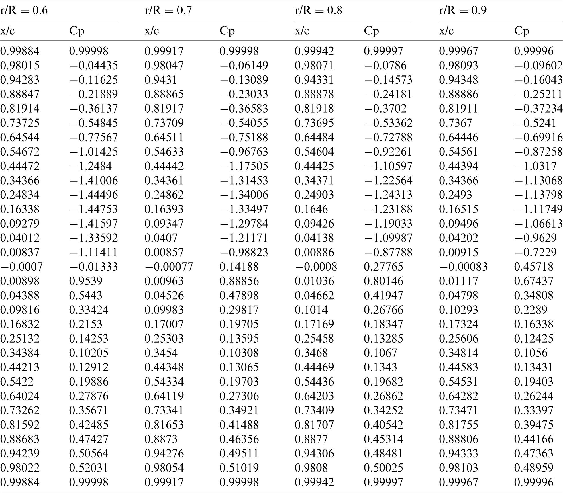
The values of Figs. 13 and 14 are tabulated, as shown in Tabs. 4 and 5:

Table 4: Power coefficient in various blade sections at the speed ratio of 7 for r/R = 0.2 to 0.5

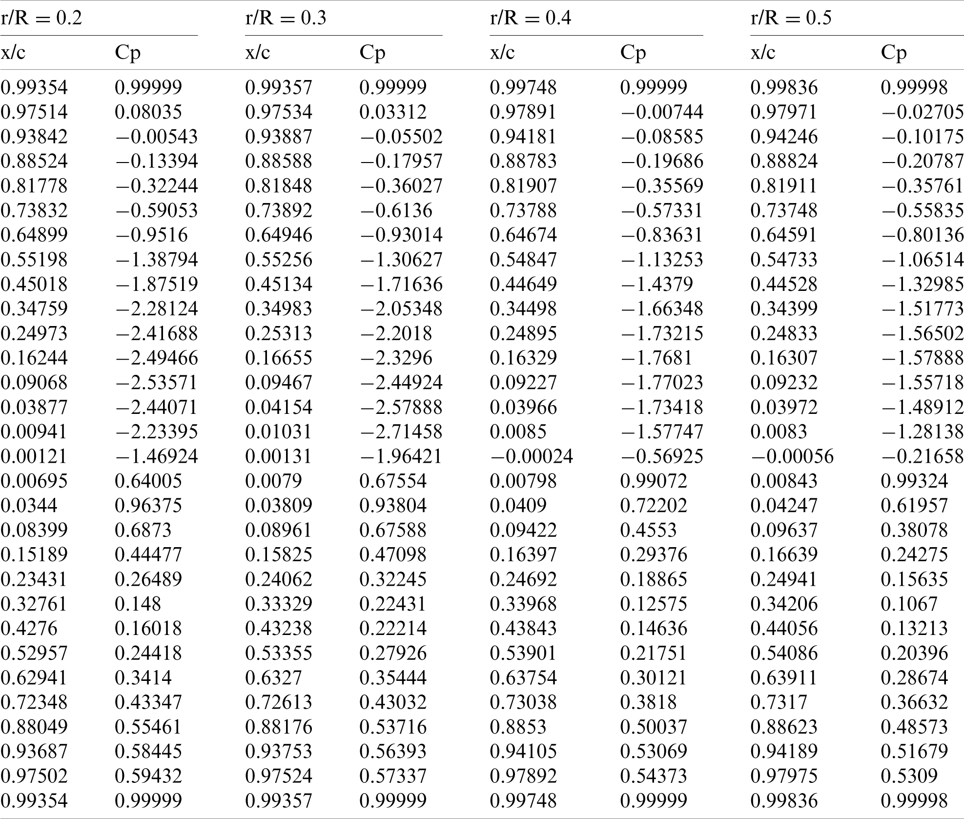
Table 5: Power coefficient in various blade sections at the speed ratio of 7 for r/R = 0.6 to 0.9

6  Conclusion

According to the present numerical study, a tidal stream turbine’s geometry has investigated using computational fluid dynamics and the blade element momentum methods. The obtained results are listed as follows:

—   The sliding-mesh technique has successfully simulated the flow through a rotational stream to a tidal turbine with a small amount of error.

—   The flow properties and the prediction of fluid behaviour are favourably obtained using the RANS method.

—   The RANS method is useful in simulating unsteady, transient turbulent flow and the prediction of wake effects, which influence the turbine farm arrangement.

—   The blade element momentum method is useful for calculating the angle of the attack coefficient at various blade sections and the axial and tangential inductive coefficients and calculating thrust force and power in tidal turbines.

—   The numerical simulations have higher accuracy than the blade momentum theory at high tip speed ratios.

It is suggested that for future research, the turbine blade’s geometric parameters can be optimized to obtain higher power in different water conditions. We can also compare the wave’s effect on a full-scale ocean turbine model by the European Ocean Energy Center data. Finally, to get more power, in a way that will be cost-effective, the economic optimization of turbines can be done by evaluating the channel’s various geometric parameters.

Funding Statement: The authors received no specific funding for this study.

Conflicts of Interest: The authors declare that they have no conflicts of interest to report regarding the present study.

This work is licensed under a Creative Commons Attribution 4.0 International License, which permits unrestricted use, distribution, and reproduction in any medium, provided the original work is properly cited.