Computer Modeling in Engineering & Sciences

DOI: 10.32604/cmes.2021.013597

ARTICLE

A Double-Phase High-Frequency Traveling Magnetic Field Developed for Contactless Stirring of Low-Conducting Liquid Materials

Xiaodong Wang1,2,*, Ernst Roland3 and Fautrelle Yves3

1College of Material Science and Opto-Electronic Technology, University of the Chinese Academy of Science, Beijing, China
2Guangwei (Zhongshan) Intelligent Technology Co., Ltd., Huairou Science City, Beijing, China
3SIMAP/EPM, Universite Grenoble Alpes, Grenoble, France
*Corresponding Author: Xiaodong Wang. Email: xiaodong.wang@ucas.edu.cn
Received: 12 August 2020; Accepted: 21 December 2020

1  Introduction

The field of magneto-hydro-energetics (MHE) couples fluid mechanics, electromagnetism and heat transfer. MHE can be applied to various electrically conducting fluid media, for example, liquid metals, electrolytes, molten oxides, ionic liquids [1–3], ionized gases or plasma. Such a field concerns various applications from astrophysics to industrial processes on a wide range of scales.

Many industrial processes involve AC magnetic fields. Induction effects are widely used in the area of processing of conducting liquid materials. The most widespread applications are induction heating and stirring of liquid metals such as steel, aluminium during their elaboration. As far as low conducting liquids are concerned, the applications deal with molten salt, electrolyte or molten glass processing. For example fluoride salts are used as electrolytes in aluminium reduction cells as well as coolant fluids in molten salt reactors [1–11]. Low conducting ionic liquids are also involved in energy storage, electrolyte materials for Li/Na batteries and biotechnology applications [2,3].

The most important advantages of induction devices are the fast heating speed, the good efficiency of the process and the absence of electrical/chemical contact and pollution between the melt and the heating device. The latter advantage is crucial when high-temperature liquids are considered.

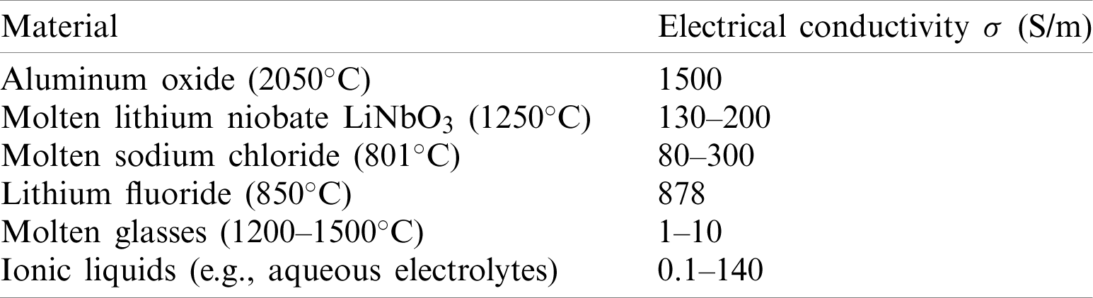
The electrical conductivity of low-conducting liquid materials is rather low, as shown in Tab. 1. Their electrical conductivity is mainly related to the mobility of ions in the bath. It may strongly depend on the temperature, e.g., molten oxides or salts, and to a lesser extent on the frequency of the applied electric currents. Efficient coupling between an AC magnetic field and a low-conducting load, i.e., heating and stirring by Lorentz forces, requires the use of high-frequency fields. Optimum coupling conditions occur when the electromagnetic skin depth is on the order of the pool diameter [1]. Specifically, the optimum coupling, both for single-phase and multiphase magnetic fields, is determined by the ratio of the electromagnetic skin depth δ to the size D of the domain, namely

δ=[1πμ0σf]1/2≈0.2-0.5D(1)

μ0, σ and f, respectively, denote the permeability of the vacuum, electrical conductivity and applied magnetic field frequency. For example, let us consider a NaCl aqueous electrolyte in a 0.3 m-diameter vessel. According to the above criterion, significant coupling is obtained when the frequency is of the order of f = 282 kHz for σ=40 S/m and δ/D≈0.5.

Table 1: Typical electrical conductivities of some materials in the liquid state [2–10]

The present publication is a continuation of preliminary works performed by Ernst et al. [4]. Its purpose concerns the design of high-frequency multiphase electromagnetic stirrers. Since multiphase generators working at high frequencies are not available, a special design of the ensemble including generator-capacitor-load is needed.

Ernst et al. [4] provided some elements in order to design a two-phase magnetic field device with several hundred kilohertz mimicking a linear motor. Ernst et al. [4] proposed the main working principle of the double oscillating circuit inductor connected to the solid-state transistor generator to form the equipment delivered by CELES Company. This technique, which yields a set of coupled oscillating circuits, consists of coupling a forced phase and an induced phase and neglects the influence of the electric parameters of the loading part (i.e., the low-conductivity liquid).

To better understand the working principle, the present work improves the previous simplified theory by taking into account a complex electrical equivalent diagram due to the different mutual couplings between the two inductors and the two corresponding induced current sets. A more detailed theoretical model is provided, and the key and sensitive elements are elaborated. Based on this theory, equipment is designed to use sodium chloride-salted water at 40 S/m to provide a stirring effect. A pure electromagnetics numerical model is presented. Numerical modelling of the load is performed in order to assess the efficiency of the stirrer with a salt water load.

The present electromagnetic model includes the two inductors coupling to the salt water-induced charge and all the electrical circuit elements connecting the two inductors to the different capacitors, connection inductances, and generator. This model is applied to a frequency sweeping study, which clearly shows the different resonance peaks corresponding to the different working resonance frequencies caught by the generator during the reception tests. Then, it is explained how the transistor generator can switch from one resonance frequency to another resonance frequency and the consequences of the two inductor currents (module difference, phase shift, etc.). Finally, in Section 4 an analytical theory based on the transformer theory is presented that is inspired by the former simplified analytical theory. It is nevertheless more complex since it takes into account the different couplings between the two inductors and the corresponding two sets of induced currents in the salt water, as in the numerical model. The latest numerical model and improved analytical model provide a better understanding of the experimental behavior of the equipment and, in turn, improved mastery of the whole process during stirring operations.

In Section 5, detailed numerical modeling of the experimental set-up is presented. It demonstrates that the traveling magnetic field is able to generate a liquid motion. This is confirmed by some experimental results obtained in a former identical installation, which consists of a salt water cylindrical tank with a diameter of 0.30 m and a height of 0.35 m (Section 6).

2  The Double-Phase Magnetic Traveling Field Stirring Installation

The installation (Fig. 1) includes a 25 kW high frequency transistor solid state converter generator feeding a set of two parallel oscillating circuits, with each consisting of a capacitor battery and an inductor. Each inductor is made of two turns connected in series-opposition, thus providing a “four-poles” magnetic field configuration. The two identical inductors, corresponding to the two electrical phases producing the magnetic traveling field, as in a linear motor, are situated with one inserted into the other, and one inductor can be shifted vertically with respect to the other so that their mutual inductance can be adjusted to reach the optimal electrical working conditions, producing equality between the two inductor current modules and 90∘ phase shift, which produces a vertical double-phase traveling magnetic field. As the transistor generator is single phased (which is the case for all high-frequency induction generators), only one oscillating circuit is connected to the generator, while the other oscillating circuit is excited by the first due to the mutual inductance between the two inductors (see, for example, Fig. 2). Finally, these two inductors are coupled to an induced charge, which is produced by low electrically conducting salt water that mimics some ionic liquids in terms of electrical conductivity (NB. Salt water is an example of ionic liquid). This salt water is contained in a 30 cm-diameter plexiglass container. A nomenclature is provided in Appendix in order to ease the reading.

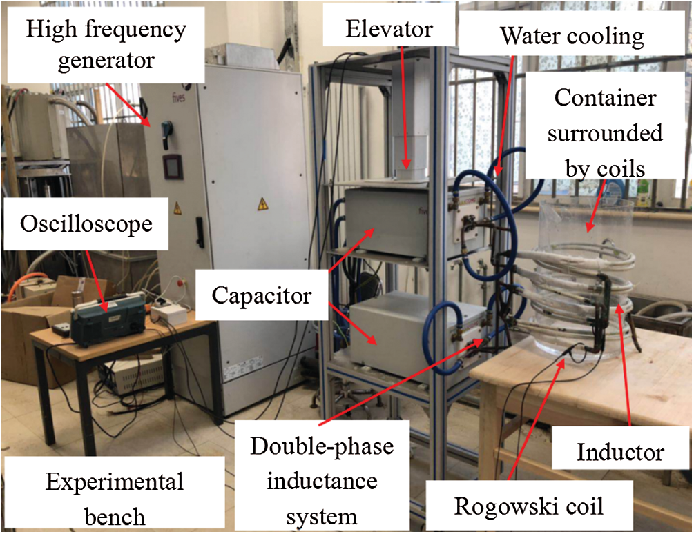
Figure 1: Double-phase magnetic traveling field stirring installation

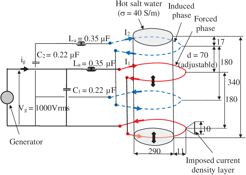
Figure 2: Simplified electrical diagram of the COMSOL model

3  Numerical Model of the Double-Phase Inductor with Connection to the Generator and Resonance Frequency Determination

The simplified electrical diagram of the COMSOLTM model is shown in Fig. 2 along the current component values from the experimental tests. The lower forced phase (in red) is connected to the generator output with a Vg=V1=1000 Vr.m.s. feeding voltage of the forced-phase inductor. Each forced and induced phase turn is a 10 mm-high current layer for the best fitting with the experimental forced and induced inductances (each of these inductance values alone (without coupling with the other, meaning that the other is an electrically open circuit) is approximately 1.55 μH). To these forced and induced inductances, two connection inductances of La=0.35 μH each are added, which gives a total inductance of each phase (L1 or L2) of approximately L=1.9μH corresponding to the experimental measurements. The two oscillating capacitors are C1=C2=0.22μF. With a vertical shift of d=70 mm (the latter value is adjustable to search the best settings), the mutual inductance M is approximately M=0.2μH, which is approximately 10% of L. The hot salt water conductivity is taken as σ=40 S/m.

The main result of frequency sweeping is displayed in Fig. 3, which shows the Ztr real part and Zti imaginary part of the global impedance Zt=Vg/ig of the whole double-phase circuit seen from the generator output for an adjustable shifting “d” distance of 70 mm, which was set for the experiment. Three possible resonance frequencies correspond to the zero crossing of Zti: f1 = 238 kHz, f0 = 252 kHz and f2 = 265 kHz. f1 and f2 are parallel resonance frequencies corresponding to a maximum of Ztr. f0 (which corresponds only to the forced phase alone the resonance frequency) is a series resonance frequency corresponding to a minimum of Ztr. The generator, owing to an internal phase-locking loop (PLL) that seeks the resonance frequencies by up-and-down sweeping, always locks onto a parallel resonance frequency, which is either frequency f1 or f2. More precisely and for the purpose of natural commutation of the transistors, the generator locks on one of two frequencies, f1′ or f2′, which are each slightly bigger than f1 and f2, and this slight shift corresponds to a capacitive behavior of Zt with a −18∘ phase shift of Vg/ig. When the adjustable distance between the two inductors becomes too big (corresponding to a mutual inductance that is too small), instability occurs, and the working resonance frequency suddenly switches from f1 (or f1′) to f2 (or f2′). As f1′ and f2′ are very close to f1 and f2, respectively, for the next calculations, we can consider that the generator works at either f1 or f2.

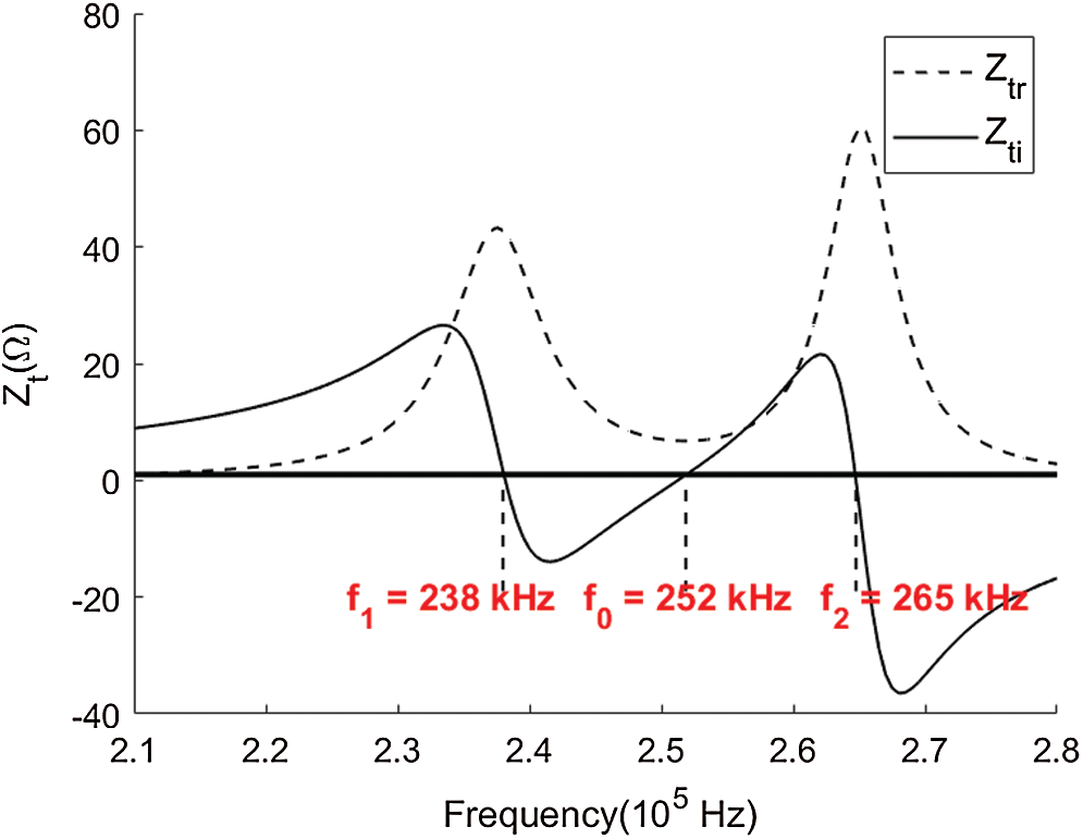
Figure 3: Real (Ztr) and imaginary (Zti) parts of the total impedance Zt seen from the generator

In Tab. 2, the main results are summarized for the three resonance frequencies, f1, f0 and f2. According to the 3rd and 5th columns, for the two resonance frequencies f1 and f2 onto which the generator locks, the I2/I1 modules ratio is close to 1, and the phase shifts of I2 with respect to I1 are respectively −20∘ and −170∘. This phase shift, even if it is small compared with the −90∘ optimal value (it will increase when the salt water becomes hotter), is sufficient to produce an upward magnetic traveling field to stir the salt water (note that this upward stirring can be reversed to downward stirring if the two phases are inversed with respect to the generator by keeping in mind that it is an asynchronous linear motor).

Table 2: Main numerical model results

4  Improved Analytical Model of the Coupled Circuits

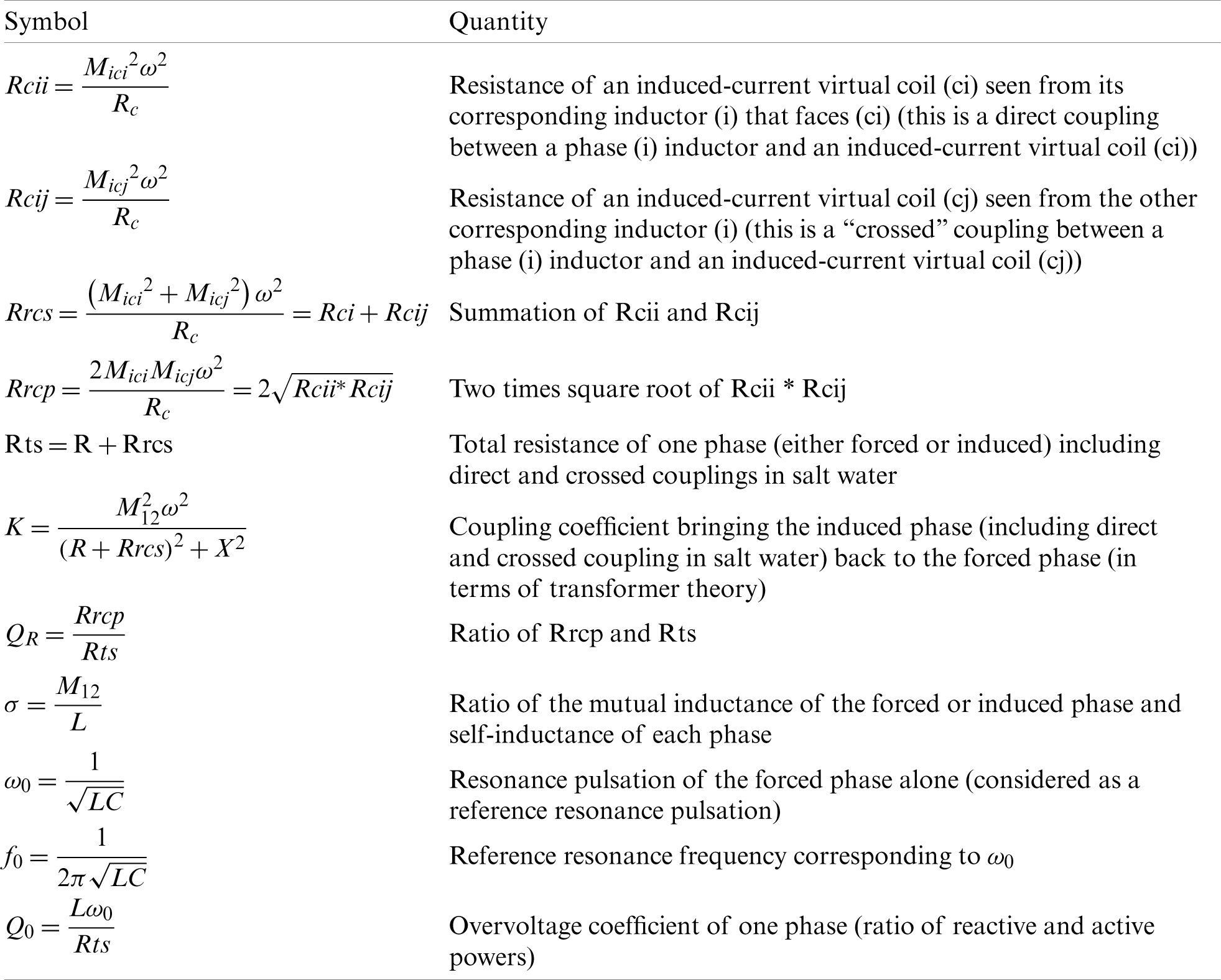
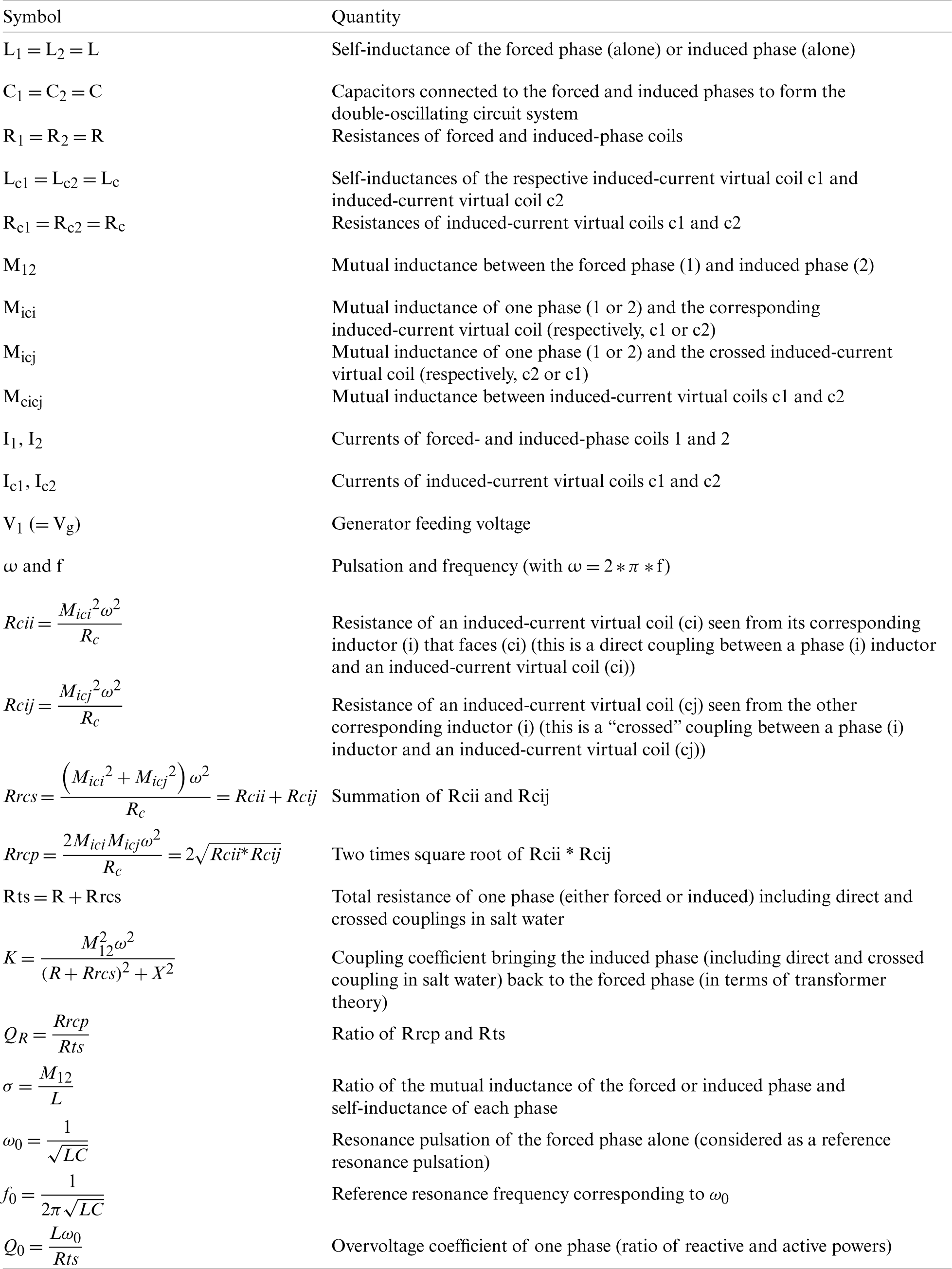
In the present model, we will take into account all the possible couplings between the two forced and induced coils and the two corresponding sets of induced currents. These two sets of induced currents can be considered as real forced and induced inductors and as virtual coils that are similar to the “images” of the real forced and induced inductors and have the corresponding resistance, self-inductance and mutual inductance relative to the other elements. This is sketched in Fig. 4, with the different couplings corresponding to the different mutual inductances defined between the inductors and induced current virtual coils (for clarity, the induced charge is set out of the inductor coils). The electrical equivalent circuit of the whole system in Fig. 2 is represented in Fig. 5. As the system is supposed to be symmetric between the forced phase and induced phase, implying that homologous parameters are the same, the magnitudes in Figs. 4 and 5 are defined in Tab. 3 (when necessary and for convenience of notation, the indices i and j are used for the forced and induced phases).

Figure 4: Sketch of the two coupled inductors and induced-current virtual coils

Figure 5: Electrical equivalent diagram of the whole double-oscillating circuit (the generator is connected to the A and B terminals)

Table 3: Definitions of electrical parameters

Without taking the C1 capacitor into account in the first state, the rest of the electrical diagram in Fig. 5 can be considered as a multi-secondary transformer whose primary is the forced-phase (1) Coil (connected to the generator) and whose secondaries are the induced-phase (2) Coil (connected to capacitor C2) on the one hand and the two induced virtual coils (connected in short circuit and coupling to all the other circuits) on the other hand.

Thus, the classical transformer equations of the system (the C1 capacitor is not yet taken into account) for the forced phase (1), the induced phase (2) and the two induced-current virtual coils are as follows:

V1=RI1+jLωI1+jM12ωI2+jM1c1ωIc1+jM1c2ωIc20=RI2+jX2I2+jM12ωI1+jM2c1ωIc1+jM2c2ωIc2 (2)

with:X2=L2ω-1C2ω=Lω-1Cω=X (3)

0=RcIc1+jLcωIc1+jM1c1ωI1+jM2c1ωI2+jMc1c2ωIc2 (4)

0=RcIc2+jLcωIc2+jM2c2ωI2+jM1c2ωI1+Mc1c2ωIc1 (5)

Eqs. (4) and (5) can be simplified because the electromagnetic skin depth in the salt water is on the same order of magnitude as the container radius; thus, one can show that Rc≫Lcω and Rc≫Mcicjω. The former four equations will be combined to obtain a general expression relating V1 to I1, which is similar to bringing back all the secondaries to the primary forced-phase coil. This gives the whole impedance Zfi(ω)=V1/I1. The purpose is to calculate the resonance pulsations ω0, ω1 and ω2 (which are, respectively, corresponding to f0, f1 and f2). As ω0, ω1 and ω2 are very close to each other, instead of the variable ω, we use a reduced variable x defined as follows: x=ωω0-ω0ω=2Δff0

Δf is the positive or negative small-frequency shift with respect to the central resonance frequency f0. Note that f0 is considered as the reference frequency corresponding to the resonance frequency of one phase alone (forced or induced phase), for which x = 0. To combine the former transformer equations into a condensed form, some specific terms are also defined in Tab. 4.

Table 4: Specific definitions of transformer equations terms

Using the notations above and assuming that ω/ω0≃1, we obtain an expression of Zfi(x) with x as the reduced variable as follows:

Zfi(x)=V1I1=[Rts+Rts(σ2Q02-QR2)-2QRσQ02x1+Q02x2]+jω[L-L2QRσ-(QR2-σ2Q02)x1+Q02x2](6)

This is the whole impedance of the forced and induced system seen from the forced-phase coil, showing the resistive part and the reactive part. By putting this impedance in parallel with the C1(= C) capacitor, we obtain the total impedance Zt seen from the generator (Zt=V1/ig=Vg/ig):

Zt(x)=T1+jT2T3+jT4(7)

with:

T1=LRtsC*[1+σ2Q02x1+Q02x2+QR-2σ+QRx1+Q02x2] (8)

T2=-Q0Rts*[1+σ2Q021+Q02x2-QRQR+2σQ02x1+Q02x2] (9)

T3=[1+σ2Q021+Q02x2-QRQR+2σQ02x1+Q02x2] (10)

T4=Q0*[(1-σ2Q021+Q02x2)x+QR-2σ+QRx1+Q02x2] (11)

The induced-to-forced-phases currents complex ratio I2/I1 can also be written with the former notation as follows:

I2I1=-(QR+σQ02x)+jQ0(σ-QRx)1+Q02x2(12)

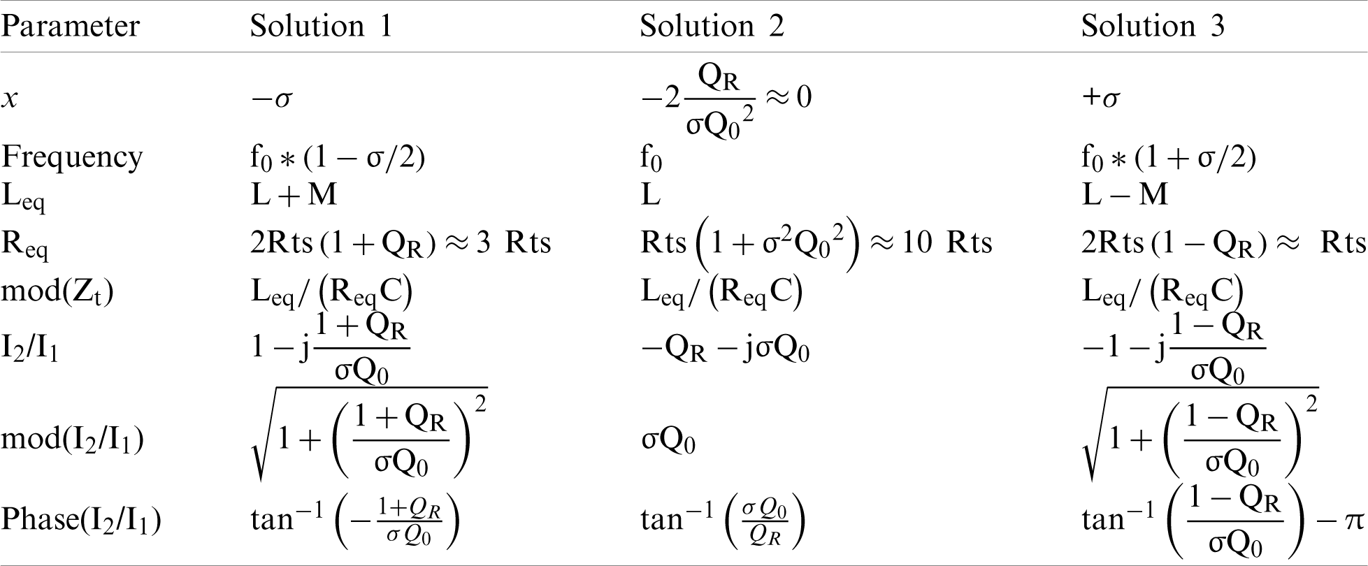
The three resonance frequencies are given by canceling the imaginary part of (7), which requires the solution of a 3rd-degree equation with the x variable. The solutions, after some simplifications due to small terms that can be neglected (this is shown in the numerical application with experimental values), are x1=-σ, x0=2QRσQ02≈0, x2=+σ, which correspond to the three resonance frequencies f1, f0 and f2, respectively. For these three solution values, we obtain a literal expression of the global equivalent inductance Leq (from the imaginary part of Zfi), global equivalent resistance Req (from the real part of Zfi), total impedance module of Zt, which can be simply deduced by mod(Zt)=Leq/(ReqC), I2/I1 currents complex ratio, module ratio and phase shift, which are summarized in Tab. 5. Note that some terms are approximated according to the experimental values.

Table 5: Main analytical calculation results

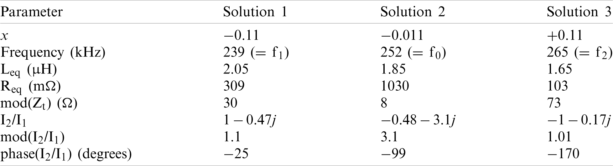
The experimental values of the different components in Fig. 5 which are obtained either from either preliminary measurements (mainly by the capacitive discharge method owing to an impedance-meter) or from the previous numerical COMSOLTM model are then applied. The main results are provided in Tab. 6. These values are for the most part very close to the homologous values in Tab. 2, which shows that the analytical model is sufficiently accurate and greatly aids in understanding the process at work. As explained previously, the generator works by locking on either frequency f1 or f2, which correspond to either −25∘ or −170∘ I2/I1 phase shift. The experiment which will be presented in the companion paper shows that after sufficient heating of the salt water, these “double-phase traveling field configuration” conditions are even improved (the I2/I1 phase shift become closer to −90∘).

Table 6: Main analytical calculation results

5  Modeling of the Magnetohydrodynamic Problem

To assess the capability of the stirring device, full magnetohydrodynamic numerical modeling is performed. Fig. 6 provides a sketch of the computation geometry, which comprises a salt water load surrounded by the two-phase coil. The geometry is 2D-axisymmetric. A widely-used Multiphysics finite-element software COMSOLTM (https://www.comsol.com/release/5.6) is used to calculate in a coupled way the magnetic field, Joule dissipation, electromagnetic forces, temperature field and electromagnetically driven flow in the load. The working parameters and physical properties are reported in Tab. 7. The detailed mathematical description of the model (equations, boundary conditions and main numerical data are summarized in Appendix 2. A transient protocol is used to calculate the flow and temperature fields, respectively from rest and room temperature. Indeed, because of the efficient Joule heating of the bath, its temperature rises quite rapidly, and the computations must be stopped before 300–400 s.

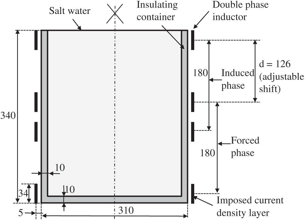
Figure 6: Sketch of the computation geometry

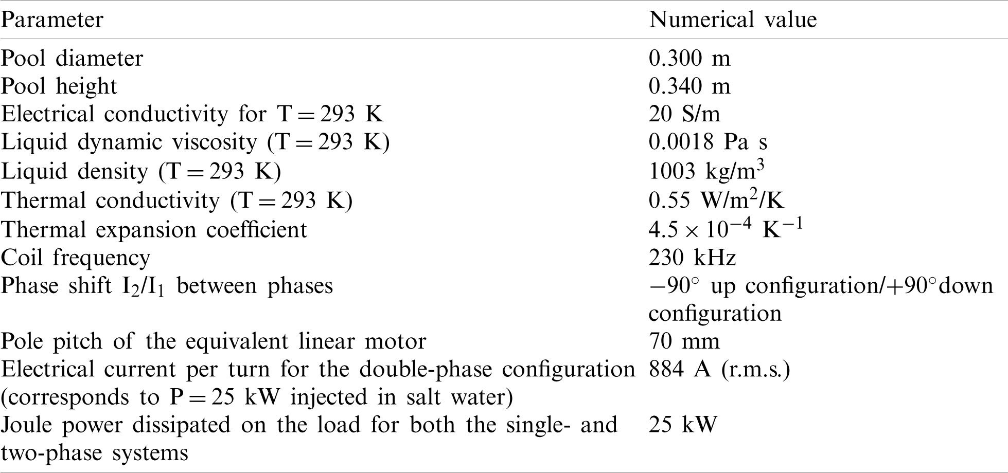
Table 7: Values of the parameters used in the computations

Numerical results are presented in Figs. 7–9. Fig. 7 shows the magnetic field distribution in the load and around the coils, whereas Figs. 8 and 9 illustrate the liquid motions. Fluid flow is generated by both electromagnetic forces and buoyancy. In both cases, the flow pattern consists of a single vortex in a meridian plane. Nevertheless, the velocity magnitudes are different. Natural convection due to Joule heating is localized mainly along the vertical walls because of the skin depth effect. Accordingly, buoyancy leads to an upward motion along the vertical walls, whereas the traveling magnetic field may be upward or downward. In Fig. 8, electromagnetic forces are oriented downward. Thus, the electromagnetic forces are opposed to buoyancy, and the velocity magnitude is less than that in the case of an upward traveling magnetic field presented in Fig. 9. Note that the maximum phase shift was used (I2/I1 phase shift imposed to −90∘ for upward configuration and +90∘ for downward configuration of the traveling field). Reaching such a value in practice is difficult.

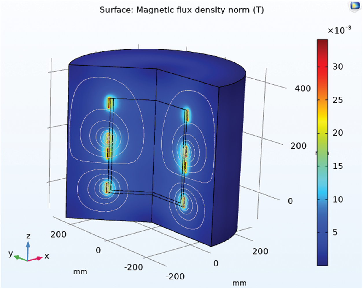
Figure 7: Magnetic field lines

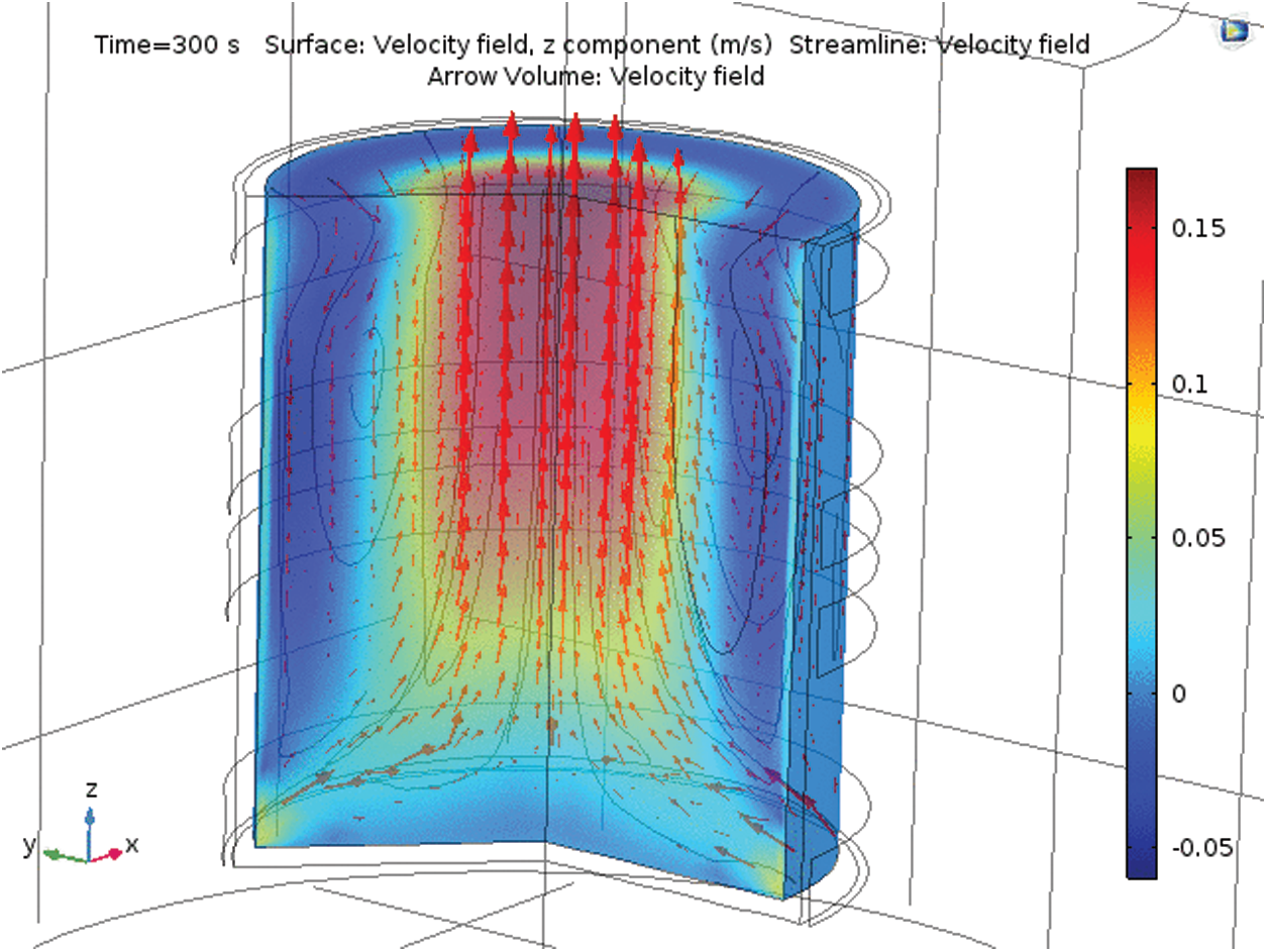
Figure 8: Flow pattern driven by both electromagnetic downward stirring and natural convection acting in opposite directions. The maximum velocity is 5 cm/s

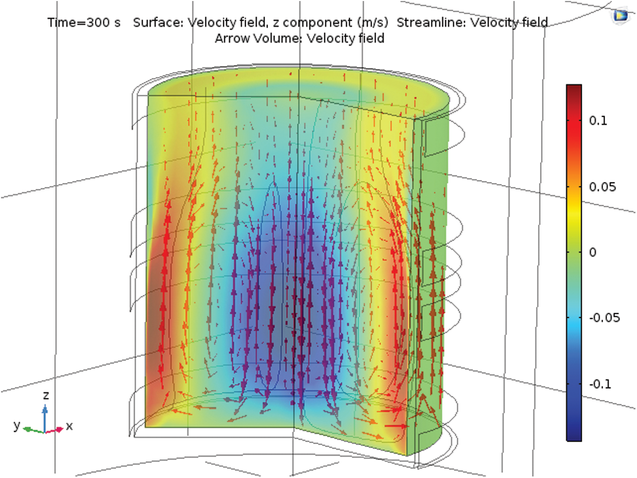
Figure 9: Flow pattern driven by both electromagnetic upward stirring and natural convection acting in the same direction. The maximum velocity is 10 cm/s

The latter results are confirmed by an analysis of the order of magnitude of the various forces and flow velocity. The typical computed magnetic flux density amplitude along the pool wall is approximately 10 mT. In the present geometry, the pole pitch is 126 mm; hence, the value of the synchronous velocity Vs is 5.8×104 m/s. The order of magnitude of the pumping body force Fem is such that [10]:

Fem=12σVsB02=116Nm3(13)

This a quite a low value compared with the liquid metal stirring forces but can be sufficient to stir an electrolyte. Indeed, balancing the fluid inertia and the electromagnetic body force provides an upper bound on the liquid velocity Uem [12], namely,

Uem=DFem2ρ=0.13ms,(14)

where ρ and D, respectively, denote density and the pool diameter.

The above estimate is in accordance with the numerical modeling. The numerical results confirmed by the analysis of the order of magnitude indicate that the electromagnetic device may be efficient in acting on a low-conducting liquid.

6  Former Experiment Results

A former similar stirring installation has been designed in 2004 [4] with the same double phase inductor connected to a triode generator working at about the same frequency. The salt water filled tank was identical to this presented in this paper. Small hollow silver coated glass spheres were immersed in the water in order to show the stirring path thanks to their tracking. To do this a vertical meridian plane in the salt water was illuminated with a vertical slot projected by a slide projector. This vertical meridian plane was then photographed with an exposure time of a few seconds thus showing the glass spheres trajectory whose length is proportional to the velocity. With the triode generator it was possible to almost reach the optimal double phase stirring conditions (mod(I2/I1) and phase (I2/I1) respectively close to 1∘ and −90∘). Fig. 10 shows the observed stirring in the enlightened meridian plane for a power level of about 6 kW injected in the salt water and a frequency of 230 kHz. Note that during the experiment a significant temperature rise occurs due to induction heating. Thus, the electrical conductivity varies from S = 20 S/m at room temperature (T=20∘C) to S = 40 S/m at the end of the experiment (T~60∘C).

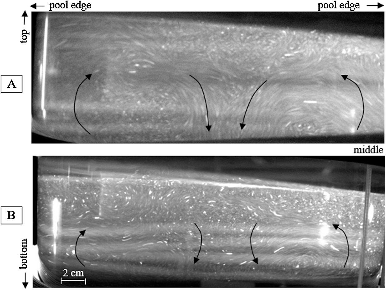
Figure 10: Photos of the bulk stirring observed in the upper half [A] and the lower half [B] of the salt water pool

The well-organized flow pattern results from additive vertical both upward natural thermo-convection and electromagnetic stirring forces in the peripheral tank area, as shown by the numerical model in Fig. 9. The longest observed spherical particles trail corresponds to a velocity of about 3.5 cm/s which shows the ability of this double phase inductor to produce an efficient stirring.

7  Conclusions and Perspective

A high-frequency traveling magnetic field apparatus has been designed. After optimizing the operating parameters, the output power of the generator can be as high as 25 kW. The power of the generator clearly dynamically changes with the impedance of the circuits. The closer the impedance of the external circuit is to the internal resistance of the high-frequency power source, the greater the output power of the high-frequency power source. The external circuit impedance varies with the distance between the two coils. Within this adjustable position range, the greater the distance is, the greater the impedance of the loop, and the greater the difference from the internal resistance of the high-frequency power source is, the higher the output power of the high-frequency power source. The impedance of the external circuit is also related to the conductivity of the salt water solution: The closer the conductivity is to 40 S/m, the closer the impedance of the circuit is to the internal resistance of the high-frequency power source, and the greater the output power of the high-frequency generator. In short, if we achieve a high output power from the high-frequency generator, then the distance between the coils should not be too large, and the conductivity of the salt water should be close to 40 S/m.

The key element in forming a traveling magnetic field is that the phase shift and amplitude ratio of the two-phase current. The phase shift of the currents is related to the distance between the coils. The greater the distance is, the larger the phase difference. It is also related to the conductivity of the load solution. The larger the conductivity of the load solution is, the larger the phase shift. The amplitude ratio of the two-phase current is related to the distance between the coils. The greater the distance is, the smaller the amplitude ratio of the two-phase current. In short, to form a traveling magnetic field, the distance between the coils should be neither too large nor too small. Note that the electrical system may sometimes be subject to instabilities linked to the tuning of the operating frequency. As far as the stirring effect is concerned, numerical modeling shows that the device is efficient enough to generate significant liquid velocities in salt water. Further experimental investigations are underway to validate the present theoretical results.

Funding Statement: This study was supported by the Instrument and Equipment Development Project of the Chinese Academy of Sciences (YJKYYQ20200053), the “Double First-Class” Construction Fund (111800XX62), and the Mechanical Engineering Discipline Construction Fund (111800M000).

Conflicts of Interest: The authors declare that they have no conflicts of interest to report regarding the present study.

References

 1.  Fautrelle, Y., Ernst, R., Moreau, R. (2009). Magnetohydrodynamics applied to materials processing. International Journal of Materials Research, 100(10), 1389–1398. DOI 10.3139/146.110187. [Google Scholar] [CrossRef]

 2.  Watanabe, M., Thomas, M. L., Zhang, S., Ueno, K., Yasuda, T. et al. (2017). Application of ionic liquids to energy storage and conversion materials and devices. Chemical Reviews, 117(10), 7190–7239. DOI 10.1021/acs.chemrev.6b00504. [Google Scholar] [CrossRef]

 3.  Egorova, K. S., Gordeev, E. G., Ananikov, V. (2017). Biological activity of ionic liquids and their application in pharmaceutics and medicine. Chemical Reviews, 117(10), 7132–7189. DOI 10.1021/acs.chemrev.6b00562. [Google Scholar] [CrossRef]

 4.  Ernst, R., Perrier, D., Brun, P., Lacombe, J. (2005). Multiphase electromagnetic stirring of low conducting liquids. COMPEL International Journal of Computations and Mathematics in Electrical, 24(1), 334–343. DOI 10.1108/03321640510571534. [Google Scholar] [CrossRef]

 5.  Khomich, V. Y., Moshkunov, S. I., Rebrov, I. E. (2016). Multiphase high-voltage high-frequency sawtooth wave generator. 2016 International Symposium on Power Electronics, Electrical Drives, Automation and Motion, Anacapri (Italy). DOI 10.1109/SPEEDAM.2016.7525962. [Google Scholar] [CrossRef]

 6.  Farahat, R., Eissa, M., Megahed, G., Fathy, A., Abdel-Gawad, S. et al. (2019). Effect of EAF slag temperature and composition on its electrical conductivity. ISIJ International, 59(2), 216–220. DOI 10.2355/isijinternational.ISIJINT-2018-507. [Google Scholar] [CrossRef]

 7.  Mills, K. C., Yuan, L., Jones, R. T. (2011). Estimating the physical properties of slags. Journal of the Southern African Institute of Mining and Metallurgy, 111, 649–658. [Google Scholar]

 8.  Han, Y. U., Min, D. J. (2016). The cationic effect on properties and structure of CaO–MgO–SiO2 melts. Advances in Molten Slags, Fluxes, and Salts: Proceedings of the 10th International Conference on Molten Slags, Fluxes and Salts. pp. 501–509. Springer, Cham. DOI 10.1007/978-3-319-48769-4_53. [Google Scholar] [CrossRef]

 9.  Courtessole, C., Etay, J. (2011). Interface, flows and transfer in an electromagnetic process devoted to liquid/liquid extraction. Advanced Engineering Materials, 13(7), 556–562. DOI 10.1002/adem.201000352. [Google Scholar] [CrossRef]

10. Zhang, S., Sun, N., He, X., Lu, X., Zhang, X. (2006). Physical properties of ionic liquids: Database and evaluation. Journal of Physical and Chemical Reference Data, 35(4), 1475–1517. DOI 10.1063/1.2204959. [Google Scholar] [CrossRef]

11. Ernst, R., Mangelinck-Noel, N., Hamburger, J., Garnier, C., Ramoni, P. (2005). Grain size reduction by electromagnetic stirring inside gold alloys. European Physical Journal Applied Physics, 30(3), 215–222. DOI 10.1051/epjap:2005019. [Google Scholar] [CrossRef]

12. Davidson, P. A. (2001). An introduction to magnetohydrodynamics. UK: Cambridge University Press. [Google Scholar]

Appendix 1

Table 8: List of symbols

Appendix 2: Mathematical Description of the Modeling of the Magnetohydrodynamic Problem

•   Physical equations and boundary conditions:

1/Electromagnetics:

—   activated in all domains (water+air)/frequency domain solver/quadratic discretization

—   Equation:

∇2A-iω(μσ+iμϵω)A+μσ(u×B)=0(last velocity term neglected)

—   with: A: Complex vector potential/u: Velocity/B: Magnetic flux density/μ: Magnetic permeability/σ: Electrical conductivity/ω: Electrical pulsation/ϵ: Permittivity

—   Boundary conditions: Outer boundaries: Magnetic insulation

2/Heat transfer:

—   activated in the water domain/time dependent solver/linear discretization

—   Equation:

Cp∂T∂t+ρCpu⋅∇T-k∇2T=Qem

—   with: T: Temperature/u: Velocity/t: Time/ρ: Density (linearized with T)/Cp: Heat capacity/k: Thermal conductivity/Qem: Volumetric electromagnetic loss density

—   Boundary conditions: Lower+side boundaries: Thermal insulation/upper boundary: Convective heat flux (heat transfer coefficient: h=10 W/(m2K)

3/Fluid mechanics:

—   activated in the water domain/time dependent solver/incompressible/laminar flow/Boussinesq approximation/P1 + P1 discretization/Streamline diffusion + crosswind diffusion (Navier Stokes equation)

—   Equations:

ρ∂u∂t+ρ(u⋅∇)u=-∇p+ν∇2u+Fem+ρgρ∇⋅u=0

—   with: u: Velocity/t: Time/ρ: Density (linearized with T)/p: Pressure/ν: Dynamic viscosity/g: Gravity/Fem: Time averaged electromagnetic Lorentz force density

—   Boundary conditions: Lower + side boundaries: No slip wall/upper boundary: Open boundary

•   Main model numerical data:

—   total number of mesh elements: 2118

—   total number of degrees of freedom: 6721

—   stored time step of dependent solver: 1 s

—   maximum Reynolds number 3800.

This work is licensed under a Creative Commons Attribution 4.0 International License, which permits unrestricted use, distribution, and reproduction in any medium, provided the original work is properly cited.