Engineering & Sciences
| Computer Modeling in Engineering & Sciences |
DOI: 10.32604/cmes.2021.014407
ARTICLE
A New Modified Inverse Lomax Distribution: Properties, Estimation and Applications to Engineering and Medical Data
Department of Statistics, Faculty of Science, King Abdulaziz University, Jeddah, 21589, Saudi Arabia
*Corresponding Author: Abdullah M. Almarashi. Email: aalmarashi@kau.edu.sa
Received: 24 September 2020; Accepted: 09 February 2021
Abstract: In this paper, a modified form of the traditional inverse Lomax distribution is proposed and its characteristics are studied. The new distribution which called modified logarithmic transformed inverse Lomax distribution is generated by adding a new shape parameter based on logarithmic transformed method. It contains two shape and one scale parameters and has different shapes of probability density and hazard rate functions. The new shape parameter increases the flexibility of the statistical properties of the traditional inverse Lomax distribution including mean, variance, skewness and kurtosis. The moments, entropies, order statistics and other properties are discussed. Six methods of estimation are considered to estimate the distribution parameters. To compare the performance of the different estimators, a simulation study is performed. To show the flexibility and applicability of the proposed distribution two real data sets to engineering and medical fields are analyzed. The simulation results and real data analysis showed that the Anderson-Darling estimates have the smallest mean square errors among all other estimates. Also, the analysis of the real data sets showed that the traditional inverse Lomax distribution and some of its generalizations have shortcomings in modeling engineering and medical data. Our proposed distribution overcomes this shortage and provides a good fit which makes it a suitable choice to model such data sets.
Keywords: Inverse lomax distribution; logarithmic transformed method; order statistics; maximum likelihood estimation; maximum product of spacing; manuscript; preparation; typeset; format
Inverse Lomax (IL) distribution is a very important lifetime distribution which can be used as a good alternative to the well known distributions such as gamma, inverse Weibull, Weibull and Lomax distributions. It can be considered as a member of generalized beta family of distributions. It has different applications in modelling various types of data including economics and actuarial sciences data because its hazard rate can be decreasing and upside down bathtub shaped. The random variable X is said to have an IL distribution if its probability density function (PDF) is
The cumulative distribution function (CDF) of (1) is
where
The main objective of this paper is to propose a new form of the IL distribution by adding a new shape parameter to the CDF in (2) using the same approach of [8]. They introduced a new method to add an extra shape parameter to an existing distributions which called the logarithmic transformed (LT) method. The LT method has the following CDF and PDF
and
respectively, with
1. To develop different shapes for the PDF and hazard rate function.
2. To increase the flexibility of the traditional IL distribution in modelling different phenomenons.
3. To model skewed data which can not be modeled by other traditional models.
4. To increase the flexibility of the traditional IL distribution properties like mean, variance, skewness and kurtosis.
5. Two applications showed that the MLTIL distribution provides a better fit than the traditional IL distribution and some of its generalizations.
6. Another motivation to this article is to use six classical estimation methods to estimate the parameters in order to recommend which method provide the best estimates based on mean square error criteria and via a simulation study.
The hazard rate function of the MLTIL distribution can has decreasing or upside-down shapes depending on its shape parameters which makes the distribution is quite effectively in modelling lifetime data. It can be used as an alternative to IL and inverse Weibull distributions. Simulation results reveal that the Anderson-Darling (AD) estimators perform better than other estimators in terms of minimum mean-squared errors. Finally, the analysis of engineering and medical data sets show the ability of the MLTIL distribution to provide a better fit than some other competitive models. The rest of the paper is organized as follows: In the next Section we describe the MLTIL distribution and a mixture representation of its density. Some of its statistical properties are discussed in Section 3. Six classical estimation methods are considered in Section 4. A simulation study is conducted in Section 5. Two applications are considered in Section 6. In Section 7, the paper is concluded.
In this section we introduce the MLTIL distribution. Let the random variable X follows the IL distribution with PDF and CDF, respectively, given by (1), (2), then from (1)–(3) the PDF of the MLTIL distribution is given by
and its CDF is
The survival function (SF) is given by
and the hazard rate functions is
For some selected values of the parameters
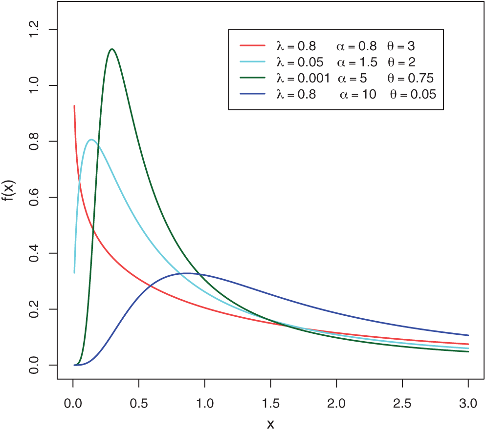
Figure 1: Plots of the MLTIL density for different values of
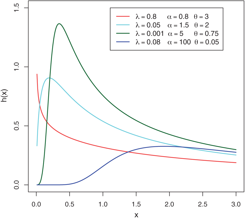
Figure 2: Plots of the MLTIL hazard rate function for different values of
Now, we can obtain an useful representation for the PDF and CDF of the MLTIL distribution. Using the series representation in the form
Applying (9) for the PDF in (1), we can obtain
where
Different structural properties of the MLTIL distribution can be determined using this representation. By integrating (10), the CDF of X is given by
where H(.) is the CDF of the IL distribution with scale and shape parameters
3 Properties of the MLTIL Distribution
In this section some statistical properties of the MLTIL distribution are obtained including quintile function, moments, incomplete moments, conditional moments and entropies.
For the MLTIL distribution the quantile function, say x = QMLTIL(q), can be obtained by inverting (6) as
We can easily generate X by taking q as a uniform random variable in
The nth moment of MLTIL distribution can be derives as
In particular,
The rth central moment
The Sk and Ku measures can be computed using the following expressions:
The following propositions are a description of three different types of moments such as incomplete moments, moment generating function (mgf) and conditional moment.
prop 3.1. If
where,
The first incomplete moment, I1(t), follows from Eq. (13) with n = 1.
prop 3.2. If
prop 3.3. If
prop 3.4. If
Entropy has been used in areas like in physics (sparse kernel density estimation), medicin (molecular imaging of tumors) and engineering (measure the randomness of systems). The entropy is a measure of variation of the uncertainty. The R
For the MLTIL distribution in (1), we can write
The
Shannon’s entropy (SE) is defined as
3.4 Distribution of Order Statistics
Let
where B(., .) is the beta function. Using (1), (6) and a power series expansion, we obtain
From (17) and (16), we can write
Particularly, we can obtain the PDF of the first and last order statistics from (18), respectively, as
and
3.5 Probability Weighted Moments
The
Based on Eq. (21), we can obtain the probability weighted moments of the MLTIL distribution as
where
3.6 Residual Life and Reversed Failure Rate Function
The nth moment of the residual life (RL) of the random variable X is defined as follows
Based on Eq. (1) and applying the binomial expansion of (x − t)n, we have
The nth moment of the reversed RL can be derived using the general formula
Based on Eq. (1) and applying the binomial expansion of (t − x)n, we can write
Let
Using series expansion in the last equation, we obtain
In this section, six estimation methods are considered to estimate the MLIIL distribution parameters.
4.1 Maximum Likelihood Estimation
Using a random sample of size m taken from the MLTIL distribution, then based on (5) the log-likelihood function can be written as
where
It is observed that these equations cannot be solved analytically for
Kao et al. [18,19] originally proposed the percentile method of estimation and recently used by many authors to obtain the parameters of some proposed distributions, see for example [20,21]. It is very useful when the distribution has a closed form quantile function. Since the MLTIL distribution has an explicit quantile function as in (12), then we can obtain the percentile estimates (PEs) of
where x(j) is the ordered observation of xj,
4.3 Maximum Product of Spacing Estimation
Cheng et al. [22,23] introduced the method of maximum product of spacing (MPS) to obtain the estimates of the continuous univariate distributions parameters as an alternative to the method of maximum likelihood. Let
To obtain the MPS estimates (MPSEs) of
with respect to
and
where
4.4 Least and Weighted Least Squares Estimation
Swain et al. [24] considered the least squares (LS) and weighted least squares (WLS) methods to estimate the beta distribution parameters. The LS estimates (LSEs) of
with respect to
4.5 Anderson-Darling Estimation
The AD method of estimation is a type of minimum distance estimator which obtained by minimizing an AD statistic. The AD estimates (ADEs) of
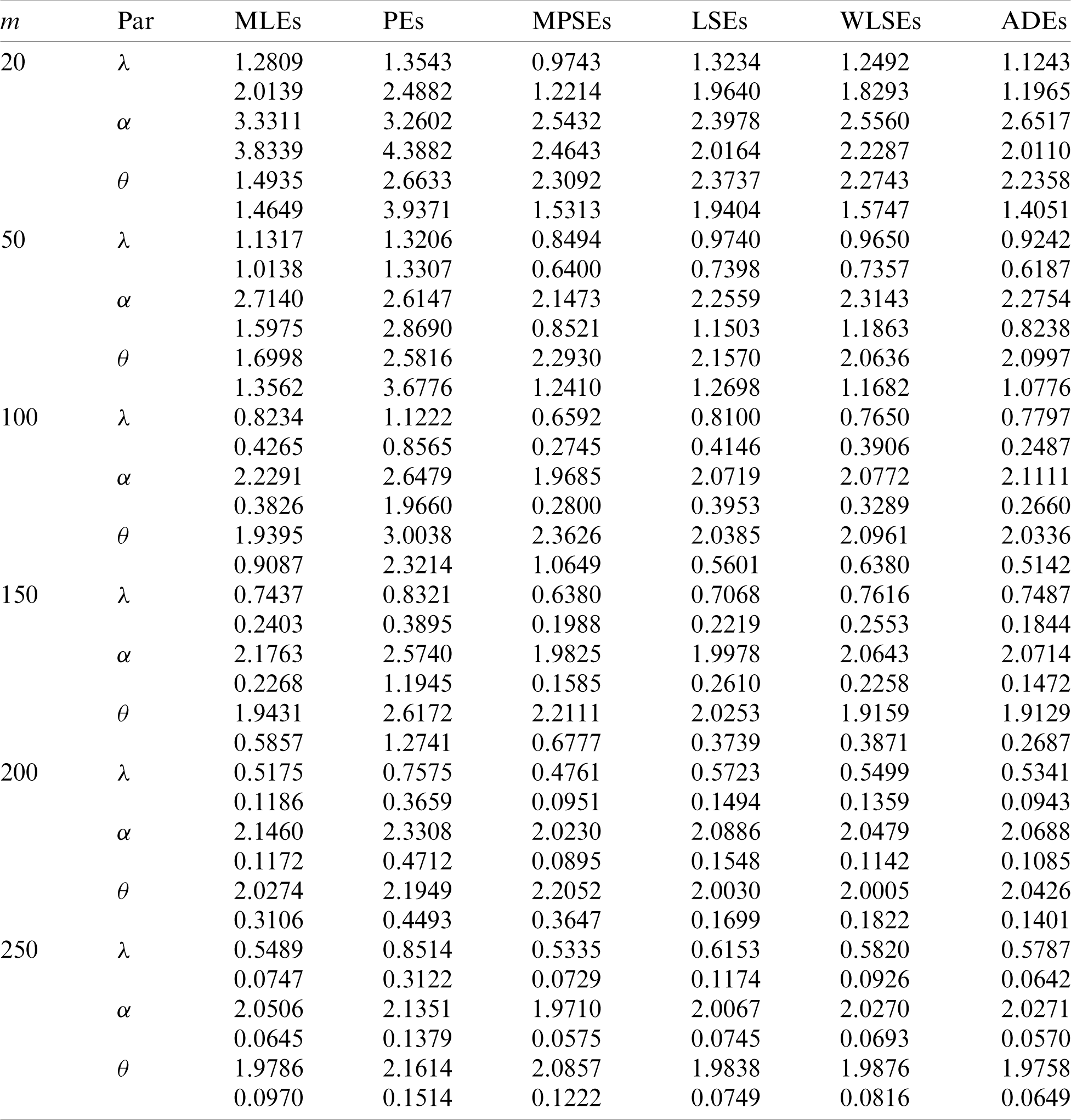
We cannot compare the performance of the different proposed estimators theoretically, therefore a simulation study is done in order to show the behavior of the various estimators in terms of mean square error (MSE) criteria. To conduct the simulation study, we choose two sets of the parameters values; Set I:
Table 1: Estimates and MSEs for different estimates of
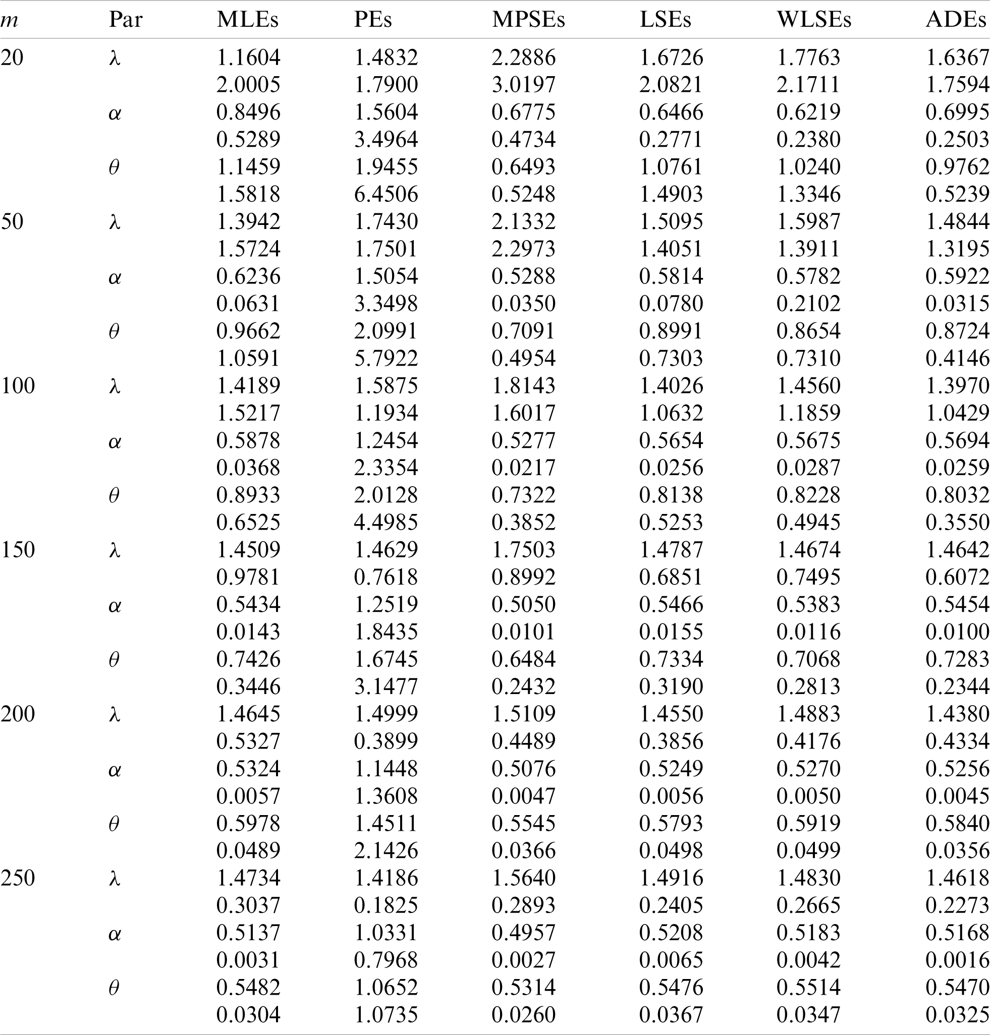
Table 2: Estimates and MSEs for different estimates of
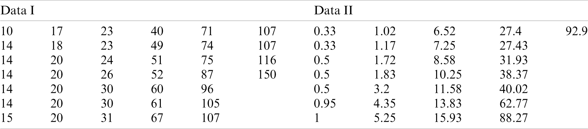
To show the applicability of the proposed distribution and the different estimators derived in the previous sections two real data sets are analyzed. The first data set considered by [25] which represent life times (in days) of 39 liver cancers patients taken from Elminia cancer center Ministry of Health in Egypt. The second data set consists of 29 time between failures of a piece of construction equipment in chronological studied by [26]. These data are displayed in Tab. 3.
We compare the results of the MLTIL distribution with IL distribution, inverse Weibull (IW) distribution, APIL distribution by [7] and alpha power inverse Weibull (APIW) distribution by [27]. The density functions of these distributions (for x > 0) are as follow
We first obtain the MLEs of the competitive distributions. These estimates are presented in Tabs. 4 and 5 for datas 1 and 2, respectively. To compare the performance of the difference distributions to fit the data set, we use Kolmogorov-Smirnov (K-S) distance and the corresponding p-value. These statistics are also presented in Tabs. 4 and 5 for datas 1 and 2, respectively. From the results in these Tables it is observed that the MLTIL distribution has the smallest K-S distance with the highest p-value among other competitive distributions, therefore we conclude that the MLTIL distribution is the suitable model to fit these data. The fitted PDF, CDF, SF and P-P plot of the MLTIL distribution are presented in Figs. 3 and 4 for datas 1 and 2, respectively. These Figures support the results discussed before that the MLTIL distribution provides a close fit to these data sets.
Table 4: MLEs, K-S and p-value of real data 1
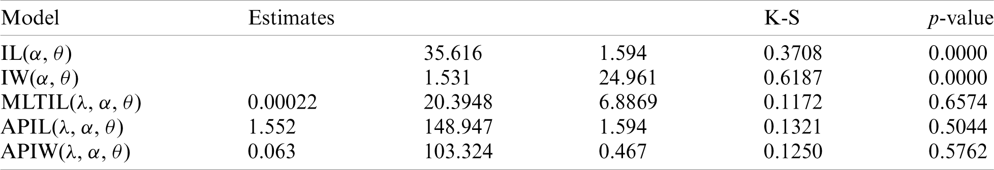
Table 5: MLEs, K-S and p-value of real data 2
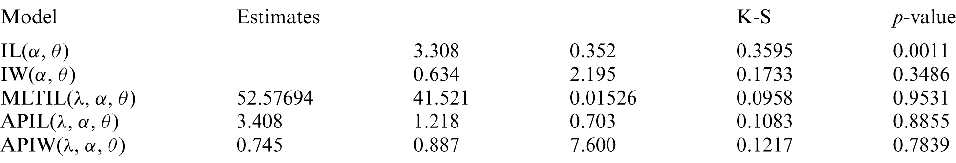
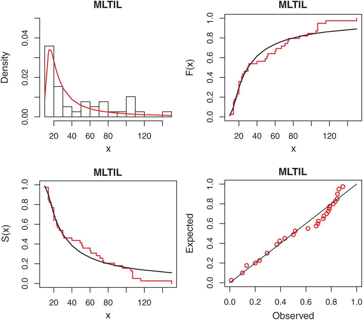
Figure 3: Fitted density, estimated CDF and SF, and P-P plots for real data 1
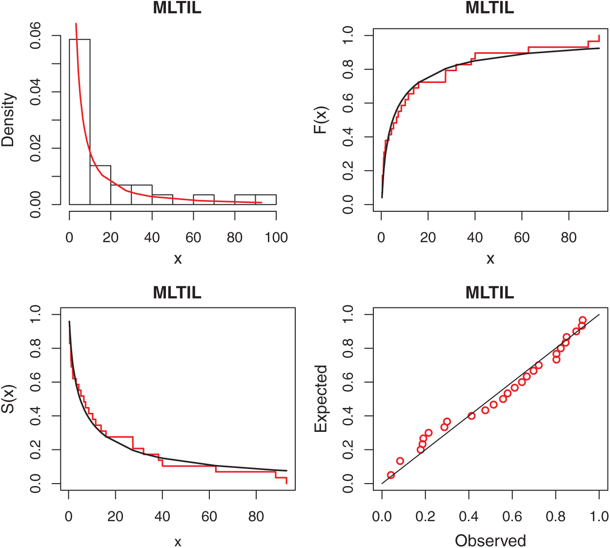
Figure 4: Fitted density, estimated CDF and SF, and P-P plots for real data 2
To see which estimation method provide a good fit to these data we compare the other estimation methods with the maximum likelihood methods based on K-S distance and its p-value. For the two data sets, the various estimates, K-S distance and its p-value are obtained in Tabs. 6 and 7, respectively. Comparing the fitting of the different methods we can observe that the ADEs provides a good fit based on minimum K-S distance with highest p-value. Therefore, we can recommend to use the AD method to estimate the MLTIL distribution parameters from these real data sets. Also, the histogram and the fitted MLTIL distribution based on the different methods are presented in Fig. 5 for the two data sets.
Table 6: Various estimates, K-S and p-value of real data 1
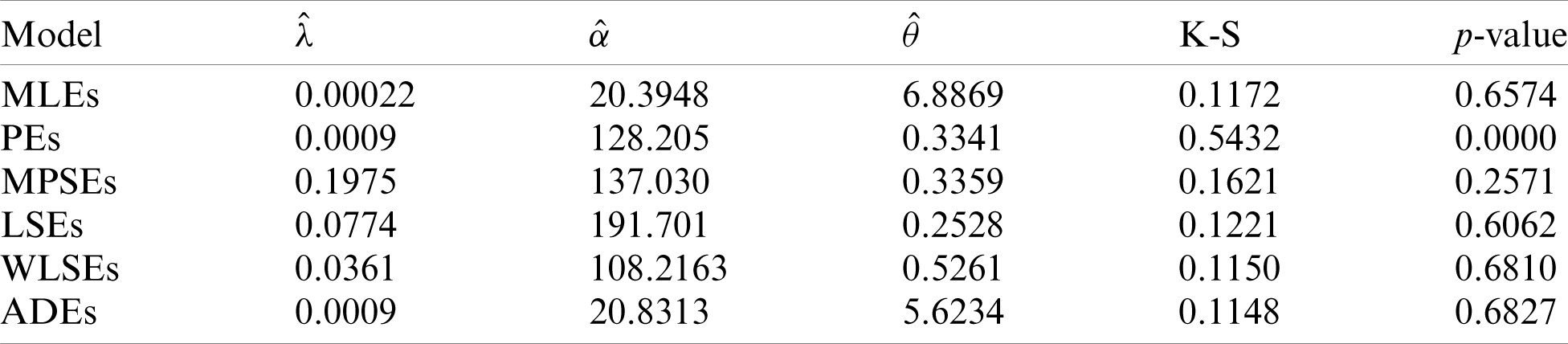
Table 7: Various estimates, K-S and p-value of real data 2
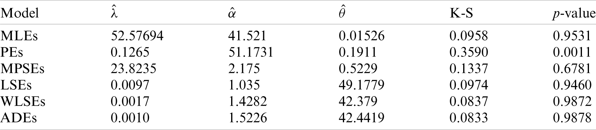
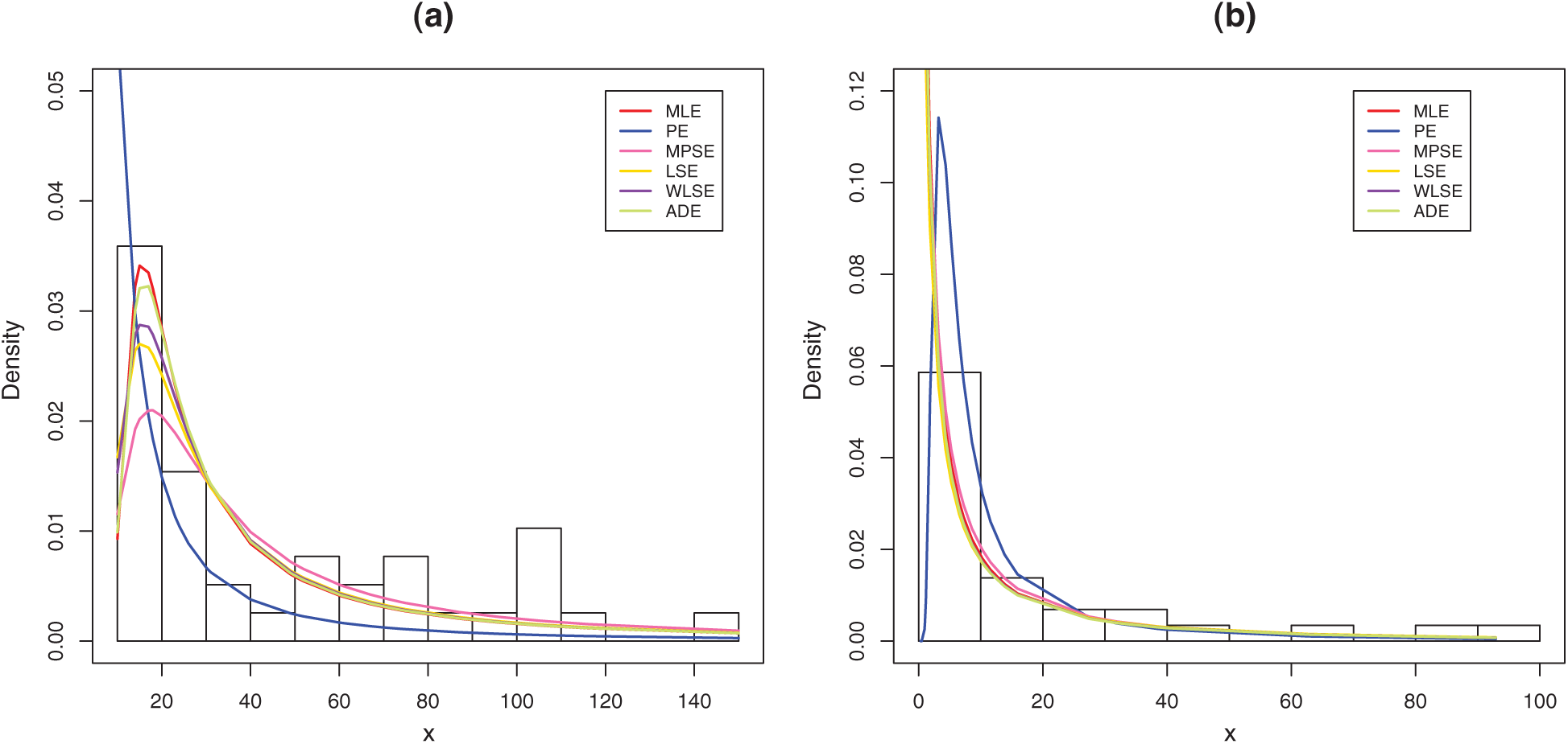
Figure 5: Histogram and the fitted MLTIL density using different estimation methods for (a) data 1 and (b) data 2
In this paper, we have considered and studied a new generalization of the traditional inverse Lomax distribution by adding a new shape parameter. We have used the logarithmic transformed method for this purpose and a new three parameters inverse Lomax distribution which called modified logarithmic transformed inverse Lomax distribution is introduced. The new distribution has different failure rate shapes, so it can be used in analyzing lifetime data. Some statistical properties of the new distribution are derived including quantiles, moments, probability weighted moments, entropies, residual life, stress-strength parameter and order statistics. To estimate the parameters of the proposed distribution, six classical methods are considered. To compare the efficiency of these methods a simulation study is performed and the performance of the different estimators is compared. To show the applicability of the new distribution, two real data sets are analyzed which indicate that our new distribution perform better than some other competitive distributions. Also, the numerical illustration revealed that the Anderson Darling estimation method is the best method to estimate the proposed distribution parameters. In this study, the proposed distribution shows its ability in modelling engineering and medical data sets where traditional and some recently proposed models cannot be used for this purpose. We hope that this model attract wider sets of applications in the other different fields.
Acknowledgement: The author would like to thank the editor and the two reviewers for their constructive comments which improve the quality of the paper.
Funding Statement: This project was funded by the Deanship Scientific Research (DSR), King Abdulaziz University, Jeddah under Grant No. (RG-14-130-41). The author, therefore, acknowledge with thanks DSR for technical and financial support.
Conflict of Interest: The authors declare that they have no conflicts of interest to report regarding the present study.
1. Louzada, F., Ramos, P. L., Nascimento, D. (2018). The inverse nakagami-m distribution: A novel approach in reliability. IEEE Transactions on Reliability, 67(3), 1030–1042. DOI 10.1109/TR.2018.2829721. [Google Scholar] [CrossRef]
2. Eliwa, M. S., El-Morshedy, M., Ibrahim, M. (2019). Inverse Gompertz distribution: Properties and different estimation methods with application to complete and censored data. Annals of Data Science, 6(2), 321–339. DOI 10.1007/s40745-018-0173-0. [Google Scholar] [CrossRef]
3. Ramos, P. L., Louzada, F., Shimizu, T. K., Luiz, A. O. (2019). The inverse weighted Lindley distribution: Properties, estimation and an application on a failure time data. Communications in Statistics-Theory and Methods, 48(10), 2372–2389. DOI 10.1080/03610926.2018.1465084. [Google Scholar] [CrossRef]
4. Hassan, A. S., Abd-Allah, M. (2019). On the inverse power Lomax distribution. Annals of Data Science, 6(2), 259–278. DOI 10.1007/s40745-018-0183-y. [Google Scholar] [CrossRef]
5. Hassan, A. S., Mohamed, R. E. (2019). Weibull inverse lomax distribution. Pakistan Journal of Statistics and Operation Research, 15(3), 587–603. DOI 10.18187/pjsor.v15i3.2378. [Google Scholar] [CrossRef]
6. Maxwell, O., Chukwu, A. U., Oyamakin, O. S., Khaleel, M. (2019). The Marshall–Olkin inverse lomax distribution (MO-ILD) with application on cancer stem cell. Journal of Advances in Mathematics and Computer Science, 33, 1–12. DOI 10.9734/jamcs/2019/v33i430186. [Google Scholar] [CrossRef]
7. ZeinEldin, R. A., Haq, M. A., Hashmi, S., Elsehety, M. (2020). Alpha power trans- formed inverse lomax distribution with different methods of estimation and applications. Complexity, 2020(1), 1–15. DOI 10.1155/2020/1860813. [Google Scholar] [CrossRef]
8. Pappas, V., Adamidis, K., Loukas, S. (2012). A family of lifetime distributions. International Journal of Quality, Statistics, and Reliability, 1–6. DOI 10.1155/2012/760687. [Google Scholar] [CrossRef]
9. Al-Zahrani, B., Marinho, P. R. D., Fattah, A. A., Ahmed, A. H. N., Cordeiro, G. M. (2016). The (P-A-L) extended Weibull distribution: A new generalization of the Weibull distribution. Hacettepe Journal of Mathematics and Statistics, 45, 851–868. [Google Scholar]
10. Dey, S., Nassar, M., Kumar, D. (2017). Alpha logarithmic transformed family of distributions with applications. Annals of Data Science, 4(4), 457–482. DOI 10.1007/s40745-017-0115-2. [Google Scholar] [CrossRef]
11. Eltehiwy, M. (2018). Logarithmic inverse Lindley distribution: Model, properties and applications. Journal of King Saud University–Science, 32(1), 136–144. DOI 10.1016/j.jksus.2018.03.025. [Google Scholar] [CrossRef]
12. Dey, S., Nassar, M., Kumar, D., Alaboud, F. (2019). Alpha logarithm transformed fréchet distribution: Properties and estimation. Austrian Journal of Statistics, 48(1), 70–93. DOI 10.17713/ajs.v48i1.634. [Google Scholar] [CrossRef]
13. Fisher, B., Kilicman, A. (2012). Some results on the gamma function for negative integers. Applied Mathematics Information Sciences, 6, 173–176. [Google Scholar]
14. Gradshteyn, I. S., Ryzhik, I. M. (2014). Table of integrals, series, and products. sixth edition. San Diego: Academic Press. [Google Scholar]
15. Akgul, A. (2020). Analysis and new applications of fractal fractional differential equations with power law kernel. Discrete Continuous Dynamical Systems-S, DOI 10.3934/dcdss.2020423. [Google Scholar] [CrossRef]
16. Atangana, A., Akgul, A., Owolab, K. M. (2020). Analysis of fractal fractional differential equations. Alexandria Engineering Journal, 59(3), 1117–1134. DOI 10.1016/j.aej.2020.01.005. [Google Scholar] [CrossRef]
17. Owolab, K. M., Atangana, A., Akgul, A. (2020). Modelling and analysis of fractal-fractional partial differential equations: Application to reaction-diffusion model. Alexandria Engineering Journal, 59(4), 2477–2490. DOI 10.1016/j.aej.2020.03.022. [Google Scholar] [CrossRef]
18. Kao, J. H. (1958). Computer methods for estimating Weibull parameters in reliability studies. IRE Transactions on Reliability and Quality Control, 13, 15–22. DOI 10.1109/IRE-PGRQC.1958.5007164. [Google Scholar] [CrossRef]
19. Kao, J. H. K. (1958). A graphical estimation of mixed Weibull parameters in life testing electron tube. Technometrics, 1(4), 389–407. DOI 10.1080/00401706.1959.10489870. [Google Scholar] [CrossRef]
20. Santo, A. P. J., Mazucheli, J. (2014). Comparison of estimation methods for the Marshall–Olkin extended Lindley distribution. Journal of Statistical Computation and Simulation, 85(17), 3437–3450. DOI 10.1080/00949655.2014.977904. [Google Scholar] [CrossRef]
21. Nassar, M., Afify, A. Z., Dey, S., Kumar, D. (2018). A new extension of Weibull distribution: Properties and different methods of estimation. Journal of Computational and Applied Mathematics, 336(1), 439–457. DOI 10.1016/j.cam.2017.12.001. [Google Scholar] [CrossRef]
22. Cheng, R. C. H., Amin, N. A. K. (1979). Maximum product of spacings estimation with applications to the lognormal distribution. Math Report, 791. [Google Scholar]
23. Cheng, R. C. H., Amin, N. A. K. (1983). Estimating parameters in continuous univariate distributions with a shifted origin. Journal of the Royal Statistical Society: Series B (Methodological), 45(1983), 394–403. [Google Scholar]
24. Swain, J., Venkatraman, S., Wilson, J. (1988). Least squares estimation of distribution function in Johnsons translation system. Journal of Statistical Computation and Simulation, 29(4), 271–297. DOI 10.1080/00949658808811068. [Google Scholar] [CrossRef]
25. Mahmoud, M. A. W., Attia, F. A., Taib, I. B. (2005). Test for exponential better than used in average based on the total time on test transform. The Proceeding of the 17th Annual Conference on Statistics, Modelling in Human and Social Science, pp. 29–30. Cairo, Egypt. [Google Scholar]
26. Fan, Q., Fan, H. Q. (2015). Reliability analysis and failure prediction of construction equipment with time series models. Journal of Advanced Management Science, 3, 203–210. DOI 10.12720/joams.3.3.203-210. [Google Scholar] [CrossRef]
27. Basheer, A. M. (2019). Alpha power inverse Weibull distribution with reliability application. Journal of Taibah University for Science, 13(1), 423–432. DOI 10.1080/16583655.2019.1588488. [Google Scholar] [CrossRef]
 | This work is licensed under a Creative Commons Attribution 4.0 International License, which permits unrestricted use, distribution, and reproduction in any medium, provided the original work is properly cited. |