Engineering & Sciences
| Computer Modeling in Engineering & Sciences |
DOI: 10.32604/cmes.2021.014690
ARTICLE
Laminar and Turbulent Characteristics of the Acoustic/Fluid Dynamics Interactions in a Slender Simulated Solid Rocket Motor Chamber
Department of Mechanical Engineering, Faculty of Engineering at Rabigh, King Abdulaziz University, Rabigh, 21911, Saudi Arabia
*Corresponding Author: Abdelkarim Hegab. Email: amhegab@kau.edu.sa
Received: 20 October 2020; Accepted: 07 January 2021
Abstract: In this paper, analytical, computational, and experimental studies are integrated to examine unsteady acoustic/vorticity transport phenomena in a solid rocket motor chamber with end-wall disturbance and side-wall injection. Acoustic-fluid dynamic interactions across the chamber may generate intense unsteady vorticity with associated shear stresses. These stresses may cause scouring and, in turn, enhance the heat rate and erosional burning of solid propellant in a real rocket chamber. In this modelling, the unsteady propellant gasification is mimicked by steady-state flow disturbed by end-wall oscillations. The analytical approach is formulated using an asymptotic technique to reduce the full governing equations. The equations that arise from the analysis possess wave properties are solved in an initial-boundary value sense. The numerical study is performed by solving the parabolized Navier–Stokes equations for the DNS simulation and unsteady Reynolds-averaged Navier–Stokes equations along with the energy equation using the control volume approach based on a staggered grid system with the turbulence modelling. The v2-f turbulence model has been implemented. The results show that an unexpectedly large amplitude of unsteady vorticity is generated at the injection side-wall of the chamber and is then penetrated downstream by the bulk motion of the internal flow. These stresses may cause a scouring effect and large transient heat transfer on the combustion surface. A comparison between the analytical, computational, and experimental results is performed.
Keywords: Acoustic waves; solid rocket motor chamber; sidewall injection; perturbation analysis; acoustic instability; turbulence models manuscript
Nomenclature
| X | Dimensionless axial length x |
| y | Dimensionless vertical length y |
| A | Aspect ratio L |
| T | Dimensionless Temperature T |
| u | Dimensionless velocity in x-Dir. u |
| ui | Mean velocity |
| u | Turbulence fluctuations |
| um | Local mean streamwise velocity |
| Cf | Friction coefficient |
| v | Dimensionless velocity in y-Dir. v |
| p | Dimensionless pressure p |
| t | Dimensionless time t |
| Et | |
| SRM | Solid Rocket Motor |
| NSCBC | Navier Stokes Characteristic Boundary Condition |
| Greek Symbols | |
| Dimensionless vorticity, | |
| Amplitude of end wall disturbances | |
| Dissipation rate | |
| Chamber natural frequency | |
| Dimensionless mass density | |
| Dimensionless forcing frequency | |
| Dynamic viscosity, Pa.s | |
| Viscous and conduction terms | |
| wp | Wave amplitude |
| Aspect ratio | |
| Subscripts | |
| os | Steady State |
| w | Wall conditions |
| n | Eigenvalues |
| 0 | First fundamentals |
| o | Reference values |
| a | Acoustic |
| v | Rotational component |
| p | Planar component |
| s | Converged steady state |
| Exponents | |
| * | Resonance conditions |
| Perturbed values | |
| , | Dimensional values |
| Nondimensional Numbers | |
| Re | Reynolds number, |
| M | Characteristics Mach number M |
| Pr | Prandtl number |
| Production rate | |
The designers of the Solid Rocket Motor (SRM) are facing several technological problems requiring expertise in diverse-sub-disciplines in order to understand the nature of the fluid flow dynamics along with the associated complex wave patterns inside the chamber/nozzle geometry of the SRM. These problems include the burning of the solid propellant and its solid mechanical properties, the chamber case, and the fluid dynamics inside the cavity, shock physics and mechanical properties of the Ammonium Perchlorate oxidizer (AP)/Hydroxyl Terminated Poly Butadiene fuel (HTPB). Moreover, these complexities are characterized by very high energy densities, extremely diverse length and time scales, complex interface, and reactive, turbulent, and multiphase flows.
In order to have a stable rocket engine with desirable performance, there are two different essential models for the reacting and non-reacting systems must be examined first. The first model is directed to study the combustion of real microscale propellant that accounts the Ammonium Perchlorate oxidizer (AP)/Hydroxyl Terminated Poly Butadiene fuel (HTPB), as in [1–3] while the second model is devoted to studying the cold model (non-reactive) that consider the unsteady fluid dynamics inside the chamber/nozzle geometry, as in [4–6]. The recent studies that account the combustion process for the propellant concluded that the proposed conditions at or near the side-wall injection of the cold models are found to be different from that that considered with the reactive ones.
As a result, the current study is conducted to develop more accurate numerical techniques combined with the Navier–Stokes Characteristic Boundary Condition (NSCBC), that used to solve the parabolized, unsteady, compressible Navier–Stokes equations at the boundaries, to examine the unsteadiness of the fluid flow dynamics in the cavity of the SRM chamber and the associated complex wave patterns and their impact on the burning of real solid propellant surfaces. NSCBC is used to specify the numerically reflected boundary conditions, in order to eliminate numerically generated reflected waves and to minimize numerical dissipation near the aft end. We try in this study to assign constant velocity injection to mimic the real variation of composite propellants with end wall disturbance that generate longitudinal acoustic waves similar to the pattern that may exist in the rocket chamber. To describe the nature of a low Mach number and weakly viscous flow field generated in a long, narrow chamber with steady side-wall mass injection and end-wall disturbances, analytical, computational, and experimental studies were conducted. The inviscid rotational steady injected flow interacts with the irrotational acoustic field to generate unsteady vorticity at the side-wall and penetrates toward the centerline by the steady transverse velocity component. The axial distribution of the vertical velocity on the side-wall is prescribed.
The experimental and theoretical approaches in [7–16] studied intensively the propagation of acoustic waves (irrotational field only) in closed or open-end tubes without consideration for the mass injection from the side-wall. These studies described the behaviour of finite amplitude waves at resonance frequencies and the effect of nonlinearity on the waveform. Erickson et al. [7] studied theoretically the behaviour of forced finite amplitude oscillations in cylindrical constant and variable area ducts whose ends are closed. Shock waves were observed in the form of saw-tooth-like waveforms in the case of constant area duct when the duct oscillated at a resonance frequency. Zapirov et al. [8] performed similar theoretical and experimental works. Merkli et al. [9] studied the thermo-acoustic effects experimentally in resonant closed tubes. Their results showed the steepness of the wave and the shock wave formation near or at the resonance frequencies.
Wang et al. [10] also studied the nonlinear oscillations in a resonance gas column. They studied both closed and open tubes. In the case of closed tubes, a shock wave appears with small limiting amplitude because of nonlinearity; in the case of an open-end, the shock wave appears intermittently. Jimeniz [11] also drew this conclusion. The effect of a convergent–divergent nozzle appended to a constant area duct on the behaviour of travelling acoustic waves was described theoretically by Sileem [12] and experimentally by Sileem et al. [13]. The wave steepness increased, and an N-type waveform was noticed for the duct that ended with a convergent-area portion.
Furthermore, for the duct that ended with a convergent–divergent area, the wave amplitude near the end of the constant portion of the duct was greater than that of the convergent part only. Seymour et al. [14] studied the acoustic wave damping from fully opened, partially opened, and fully closed gas columns. They described the wave pattern at resonance conditions. They found that for a fully opened tube, the wave damping comes from the energy radiation into the adjacent medium. In the case of closed-end tubes, no energy radiates outside of the tube and, in turn, a shock wave is formed. In the case of a partially opened end tube, part of the acoustic energy is radiated, which prevents shock wave formation. Disselhorst et al. [15] and Garcia et al. [16] have conducted similar experimental and theoretical studies.
The interaction between the propagation of acoustic waves in closed or open-end tubes with mass injection from the side-wall has been studied by Staab et al. [17], Rempe et al. [18] and Zhao et al. [19]. These studies oadopt the perturbation theory in order to include the unsteadiness of the mass addition from the injection surfaces of the simulated combustion chamber as a source of the complex wave pattern inside the chamber. These generated waves are travelled in low axial Mach number (M), high Reynolds number (Re) mean flow. They concluded that the interaction between the propagated acoustic waves and the mass injection adjacent to the wall causes transverse rotational flow field and transverse temperature gradients to be clearly seen at or adjacent to the side-wall. These vorticities and the heat transfer generations may penetrate toward the centerline of the chamber and finally fill the whole domain. Moreover, their results proved that the nondimensional acoustic axial velocity component is found to be O(1) and the temperature disturbance is proportional to the Mach number with an amplitude of O(M) for
Moreover, several investigators developed a competitive linear model, as in Flandro [20] and Xuan et al. [21]. The velocity and vorticity dynamics were emphasized. They considered irrotational (acoustic) velocity and pressure disturbances, to the exclusion of rotational flow (vorticity) transients. Moreover, these studies developed a competitive linear theory to demonstrate that accurate descriptions of internal flow dynamics frequently require the presence of coexisting rotational and irrotational velocity fields systematic nonlinear asymptotic modelling were developed by Staab et al. [17] and Zhao et al. [19].
Vuillot et al. [22] and Smith et al. [23] examined the presence of similar rotational flow fields using a computational solution to the Navier Stokes equation. The acoustic disturbances are generated by imposed pressure variations along an axial location. Tseng et al. [24] and Chu et al. [25] extended related computational studies with the reaction model to account for the generated real diffusion and premixed flames adjacent to the combustion surface. The temperature variations observed in these studies arise from flame zone effects, rather than the acoustic disturbance-injected fluid interaction mentioned previously. Experimental observation by Vetel et al. [26,27] supported the concepts of vorticity generation featured by Hegab et al. [28,29].
Many investigations to chamber flow turbulence modelling, based on
Studies by Rempe et al. [18], Zhao et al. [19], and Flandro [20] have shown that inadequate treatment of boundary conditions may cause excessive numerical diffusion and, in turn, may result in an inaccurate solution or the complete elimination of small-scale phenomena.
Therefore, in this study, careful attention has been paid to the employment of modern algorithms based on higher-order accuracy techniques to solve the parabolized, unsteady, compressible Navier–Stokes equations at the boundaries. A boundary condition treatment method, namely, Navier Stokes Characteristics Boundary Condition (NSCBC), is used to specify the numerically reflected boundary conditions, in order to eliminate numerically generated reflected waves and to minimize numerical dissipation near the aft end. This technique shows that low dispersion errors and in turn, significant improvement over the old methods, e.g., extrapolation and partial use of Riemann invariant. The current study is conducted to develop more accurate numerical techniques combined with NSCBC to examine the unsteady flow field dynamics inside the solid rocket motor chamber and the associated complex generated wave and vorticity patterns and their impact on the burning of real solid propellant surfaces. Here, the analytical solutions for the steady and unsteady flow regimes are derived using the asymptotic techniques.
Moreover, in the present study, the turbulence characteristics of the induced flow inside the chamber are studied numerically. The numerical model was specially developed for this study in FORTRAN environment using our programmed code. The developed model was validated using a wide range of computational fluid dynamics (CFD) problems in different aerodynamics applications with reacting and non-reacting flows [34]. The study also presents RANS equations for time-dependent, compressible turbulent flows along with the implemented turbulence model. In addition, the numerical procedure and associated boundary conditions are explored. Moreover, an experimental solution in our recent studies [35] is adapted to validate the current computational approach.
2 Mathematical Formulation for Laminar Flow
The nondimensional conservation form of the unsteady, two dimensional, complete Navier–Stokes equations describing both fluid dynamics and acoustics in a perfect gas within a rectangular chamber can be written as follows:
where Q, E, and F are column vectors given by
With the aid of the equation of state for a perfect gas
The nondimensional properties can be written as
2.1 Initial and Boundary Conditions
For
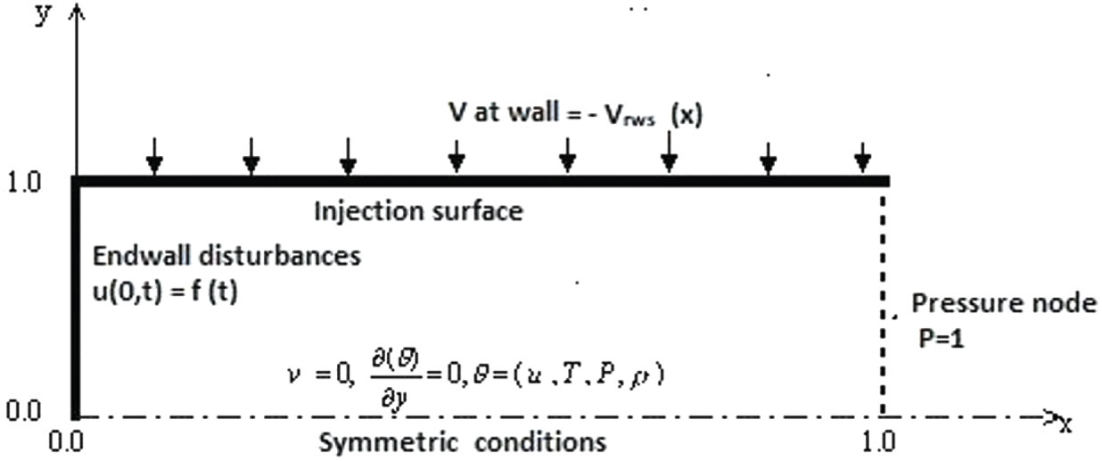
Figure 1: The physical model for the non-reactive solid rocket motor nozzle-less chamber
The boundary and initial conditions are written as follows:
The steady-state flow is generated by constant side-wall injection speed and is used as an initial condition for the unsteady flow computations. The analytical velocity profiles for incompressible, inviscid, rotational flow in a long narrow duct are used as starting profiles for the steady, compressible, viscous flow computations. The steady-state variables for the incompressible, inviscid, rotational flow can be described using the asymptotic expansions as
The asymptotic theory by Zhao et al. [19] proves that the primary viscous stresses are in the transverse direction and, as a result, the axial transportation terms can be neglected in the full Navier–Stokes equations. Eqs. (10) and (11) can be used in Eq. (1) to obtain the following equations describing an incompressible, inviscid, rotational flow:
which are valid for the limit M
The boundary conditions are
Isothermal wall with no-slip boundary conditions and side-wall injection are specified at the side-wall.
The solution to the first-order calculations in Eqs. (12)–(14) that satisfies the boundary conditions in Eqs. (15)–(19) can be written as
where Vw(x) is an arbitrary time-independent sidewall injection distribution. The solution with constant sidewall injection velocity is
To ensure that the solution converges with the steady state, the mass conservation is examined through
where
2.2.2 Unsteady Flow for Irrotational Planar Component
In this study, let the initial conditions for the unsteady flow variables
Inserting Eqs. (27) and (28) in Eq. (1), the resultant planar acoustic equation for the order of Mach number O(M) terms can be written as follows:
with the following initial and boundary conditions:
Since the left boundary condition in Eq. (31) is nonhomogeneous, the following transformation equation
With the new initial and boundary conditions
Assume the homogeneous solution for Eq. (33) is represented by
where
Then, the final non-resonance solution for the homogeneous and non-homogeneous wave equation that describes the acoustic velocity fields is derived from the summation of Eqs. (37) and (38):
The resonance solution when
Hegab [26] and Zhao et al. [19] described the irrotational acoustic system that was employed by Flandro [20] and showed that the rest of the planer irrotational functions
In this study, the experimental measurement is constructed to record only the pressure acoustic fields at several locations along the chamber. For comparison considerations, the pressure equation can be derived from Eqs. (39) and (41), considering the pressure node (P = 1) boundary conditions at the exit of the chamber. The final pressure equation for the non-resonance case is derived and written as
Consequently, the final pressure equation for the resonance acoustic equation is derived as
Also, the thermal, acoustic field for the non-resonance and resonance solution is derived and written as follows:
• For non-resonance solution
• For resonance solution (n = n*),
Moreover, the perturbed density field is determined from
Multidimensional, rotational, transient flow-dynamics in a simulated SRM chamber model are obtained from the solutions to the mass, momentum, and energy conservation equations. Numerical simulations are used to identify the acoustic fluid dynamics interactions as well as to evaluate the vorticity distribution as a function of time and space. The Two-Four explicit scheme, combined with the Navier–Stokes Characteristic Boundary Condition (NSCBC) and higher-order accuracy technique at the symmetry line, is developed to obtain a solution to the unsteady, compressible Navier–Stokes equations in the SRM chamber model as in [36–38]. This method applied recently in [39] and found to be phase accurate and therefore, suitable for describing many wave cycles and wave interaction problems.
Using the NSCBC techniques, the fluid-dynamics equations can be written in nondimensional wave modes form as follows:
where
2.3.1 Exit Boundary Conditions
In this case, the amplitude of the reflected wave based on the prescribed pressure node at the exit boundary should be
and the remaining conditions are
The nondimensional equations can be written as follows:
2.3.2 Head End Boundary Condition
The velocity component normal to the boundary (u (0, y, t)) is non-zero since the head end is the moving boundary. Thus,
The left-running wave
and the remaining amplitudes are
The wave-mode forms of the Navier–Stokes equations are simplified by ignoring the axial transportation terms in (
The nondimensional equations can be written in the form:
The nondimensional primitive variables (
More details about the NSCBC techniques are found in [28].
The accuracy of the current explicit numerical schemes has been justified by Courant–Friedrichs–Lewy (CFL) as in MacCormack [37]. They derived the following criterion to determine the size of the time step:
3 Mathematical Formulation for Turbulent Flow Characteristics
The features of the flow field are essentially transient, weakly viscous and contain vorticity distribution that has a length scale small compared to the overall geometry. These flow characteristics have similar behaviour of the turbulent flow. In this sense, the objective of this section is utilized to examine the relationship between results of the traditional studies of turbulence in injection driven channel and those found in the DNS as in Section 2.
The governing conservation equations of the flow can be written for time-dependent, compressible, and turbulent flow in the dimensional form as follows:
Continuity Equation
Momentum Equation
Energy Equation
where ui denotes the mean velocities,
The momentum equations contain additional terms, known as Reynolds stresses, which represent the effects of turbulence. These Reynolds stresses,
The Reynolds-averaged conservation Eqs. (71), (72), and (73) for unsteady compressible turbulent flow along with a turbulence model are integrated with the equation of state
In industrial CFD applications, RANS modelling remains one of the main approaches when dealing with turbulent flows. The Reynolds-averaged approach to turbulence modelling requires appropriate modelling of the Reynolds stresses in Eq. (72). The conventional method to relate the Reynolds stresses to the mean velocity gradients is based on the Boussinesq hypothesis [40]:
where
For the calculation of the turbulent viscosity, the v2-f well known turbulence model is applied. The distinguishing feature of the v2-f model is its use of the velocity scale, v2, instead of the turbulent kinetic energy, k, for evaluating the eddy viscosity. The v2, which is the velocity fluctuation normal to the streamlines, provides the proper scaling in representing the damping of turbulent transport close to the wall.
This model requires the solution to three transport equations, where the transport equation of the turbulent kinetic energy and its dissipation rate can be written as follows [41]:
where P
where S is defined as follows:
The turbulent viscosity is given by the following:
The constants of the model are given in as follows:
The importance of the turbulence studies with the aspect ratio of twenty, which is not large enough to enable a fully turbulent mean flow to develop in the chamber, suggests that the DNS may provide a better understanding for the impact of the transverse movement of the vorticity peak on the behaviour of the erosive burning.
The experimental setup layout is shown in Fig. 2. It consists of the following parts:
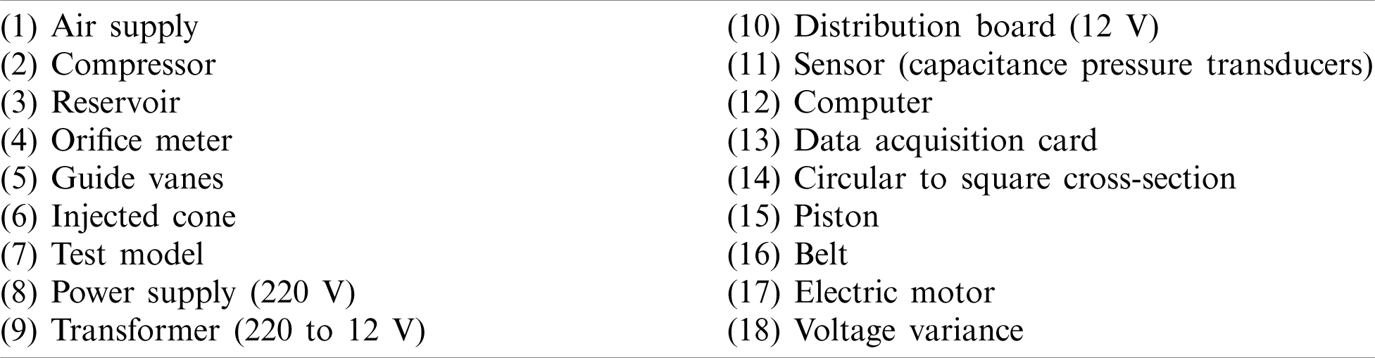
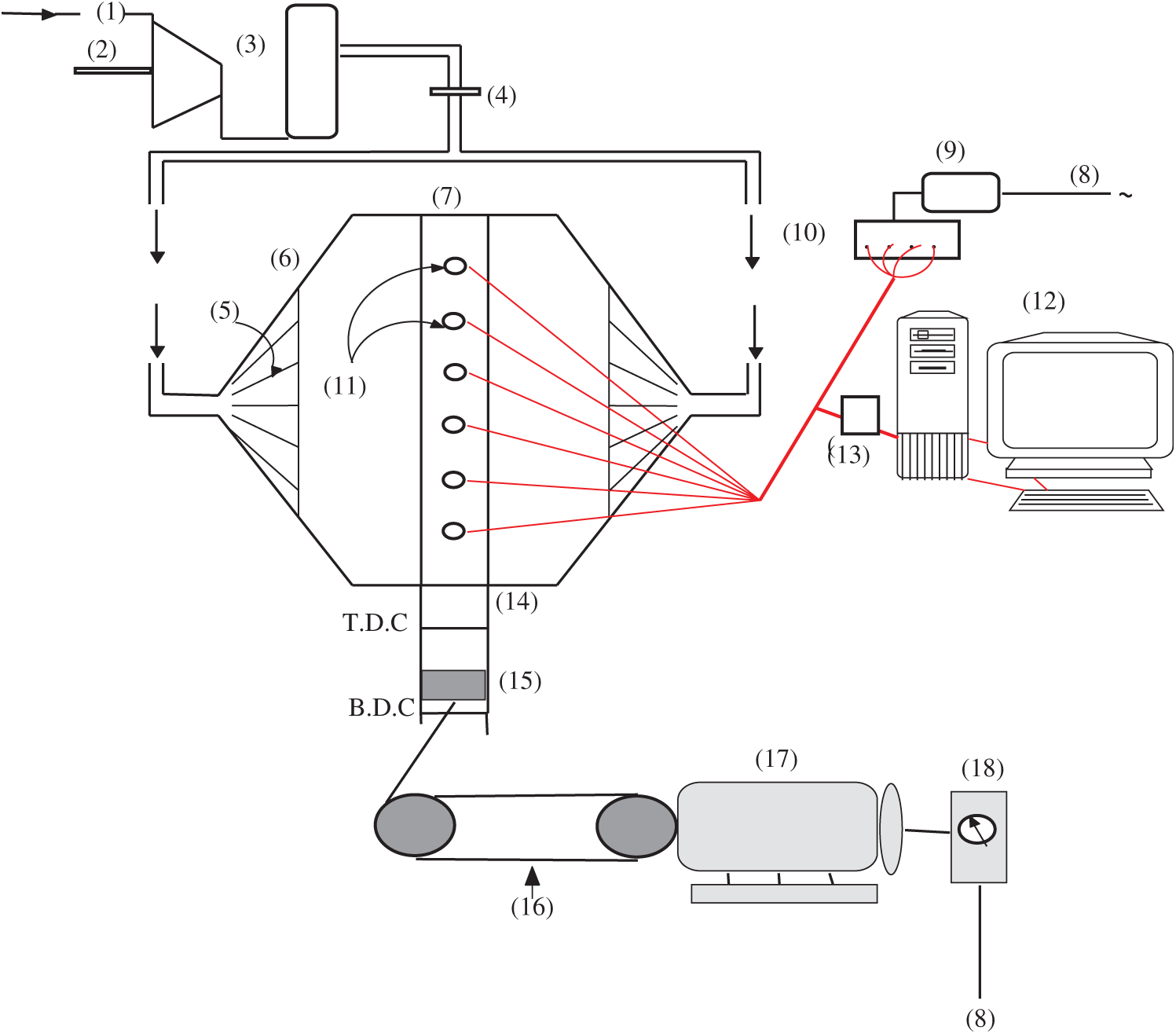
Figure 2: The layout of the test rig [35]
The piston oscillates at the head end of the tube. The acoustic pressure fields are recorded at several locations along the tube by capacitive pressure transducers (11). These transducers are connected to a computer through a built-in data acquisition system (13). The motor frequencies are changed using voltage Varies. The range of the generated frequencies from the available devices is small enough to catch the first natural frequencies (250 Hz). The pressure traces at
In this study, the asymptotic methodologies are combined with numerical and experimental approaches to give precise fundamental insights for the unsteady flow dynamics in a chamber with end-wall disturbances and steady side-wall injection. The complete axial flow speed may be divided into three parts, as by Staab et al. [17]:
where, us refers to the converged steady flow-field, which is used as an initial condition for the unsteady computations. The planar part of the flow-field, up, which describes weakly viscous acoustic effects, is created by the difference between the unsteady and the steady axial speed at y = 0, where the rotational part uv (0, t) = 0 is established from the boundary conditions. The unsteady rotational part uv is found from Eq. (84) as the difference between the total unsteady speed and the calculated us and up.
The total dimensionless unsteady vorticity is
where the vorticity is non-dimensionalized as follows:
where primed quantities are dimensional. The transverse speed component vv is found from
The parameters used to define the internal flow field include the characteristic flow Mach number (M), injection Mach number Mi = M/
Once a converged steady-state solution is established at given values of M, Re, and A, the flow is disturbed by adding transient side-wall injection with
The current results pertain to the pure planner irrotational acoustic waves and the rotational fluid flow as described in the following paragraphs.
5.1 Acoustic and Viscous Flow Dynamics in an Impermeable Duct
The first category of the results deals with the acoustic fields in the chamber without injection from the side-wall using the experimental, computational, and analytical approaches. The analytical results are obtained to describe acoustic and viscous flow dynamics in an impermeable duct when an end-wall disturbance is used to derive axial waves. The results are used to show that resonance between forced and propagating acoustic wave modes may be a source of large acoustic instability as well as to assert how nonlinear effects alter the energy in acoustic eigenfunction. The experimental results are compared with computational results to validate the numerical technique.
The first set of the results shows a comparison between experimental and computational pressure traces at x = 0.125,
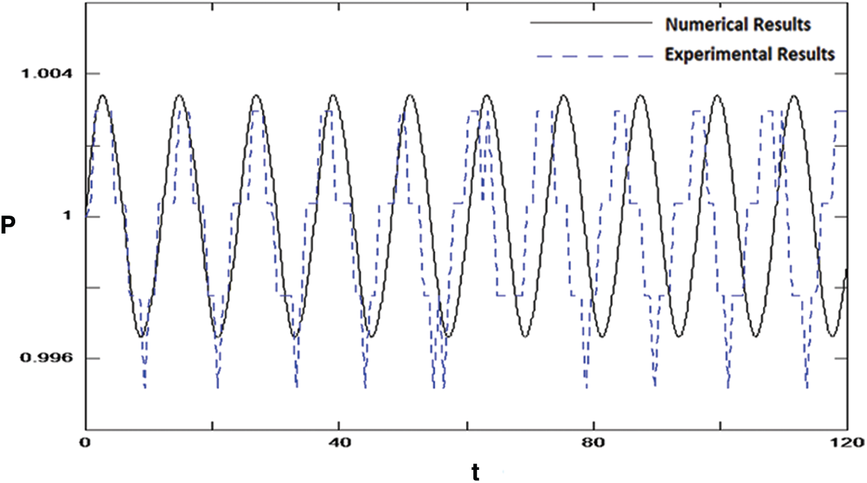
Figure 3: Comparison between the experimental and computational results for the pressure-time history at
The result illustrates the wave oscillations (quasi-steady wave motion) after many wave cycles. A stable or bounded solution is observed at this frequency. A reasonable comparison between the experimental and computational approaches is noticed. The deviations are directed to the linearity and complexity of the experimental test rig design. As a result, undesirable harmonics are seen with the experimental work due to some leaks it the connection between the circular portion of the piston and the duct shape.
In the current study, the computational and asymptotic approaches are extended to cover a wide range of frequencies away from the first fundamental mode (
Moreover, the pressure-time history at the mid-length of the chamber for
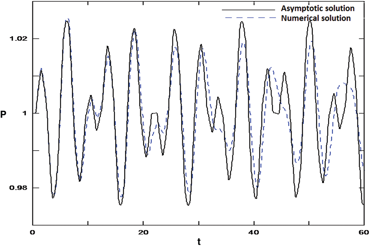
Figure 4: Comparison between the computational and analytical results for the pressure-time history at the mid-length of the chamber,
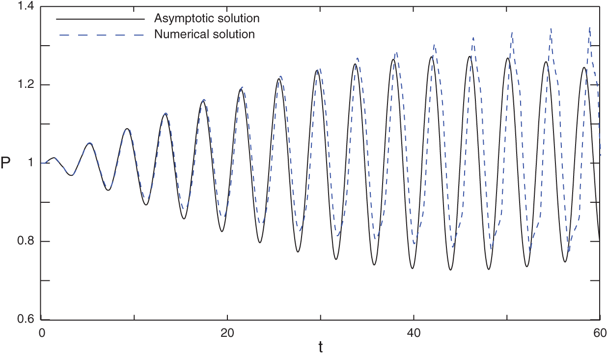
Figure 5: Comparison between the computational and analytical results for the pressure-time history at the mid-length of the chamber,
It is noted that the frequencies increase as time increases for both pressure and velocity fields when the forced frequency (
Coupling effects between the burning process and the flow characteristics inside the SRM chamber are associated with small-amplitude pressure oscillations, which can be described mathematically in terms of appropriate eigenfunctions. The co-existence of forced acoustic modes and propagating modes has a significant role in the energy exchange mechanism and acoustic instability inside the chamber of an SRM. One of the primary objectives of this research is to illustrate how acoustic wave patterns in a duct are generated by a simple time-dependent boundary condition at the head end in terms of an initial-boundary value formulation. The numerical solution to the full parabolized nonlinear, unsteady, compressible Navier–Stokes equations is integrated with the analytical solutions using the perturbation theory to the weakly nonlinear analysis of the acoustic waves to examine the complex acoustic/fluid dynamics mechanism and their impact on the combustion of real solid fuel. Moreover, both approaches are used to show that the resonance between forced and propagating acoustics wave modes may be the source of large acoustic instability.
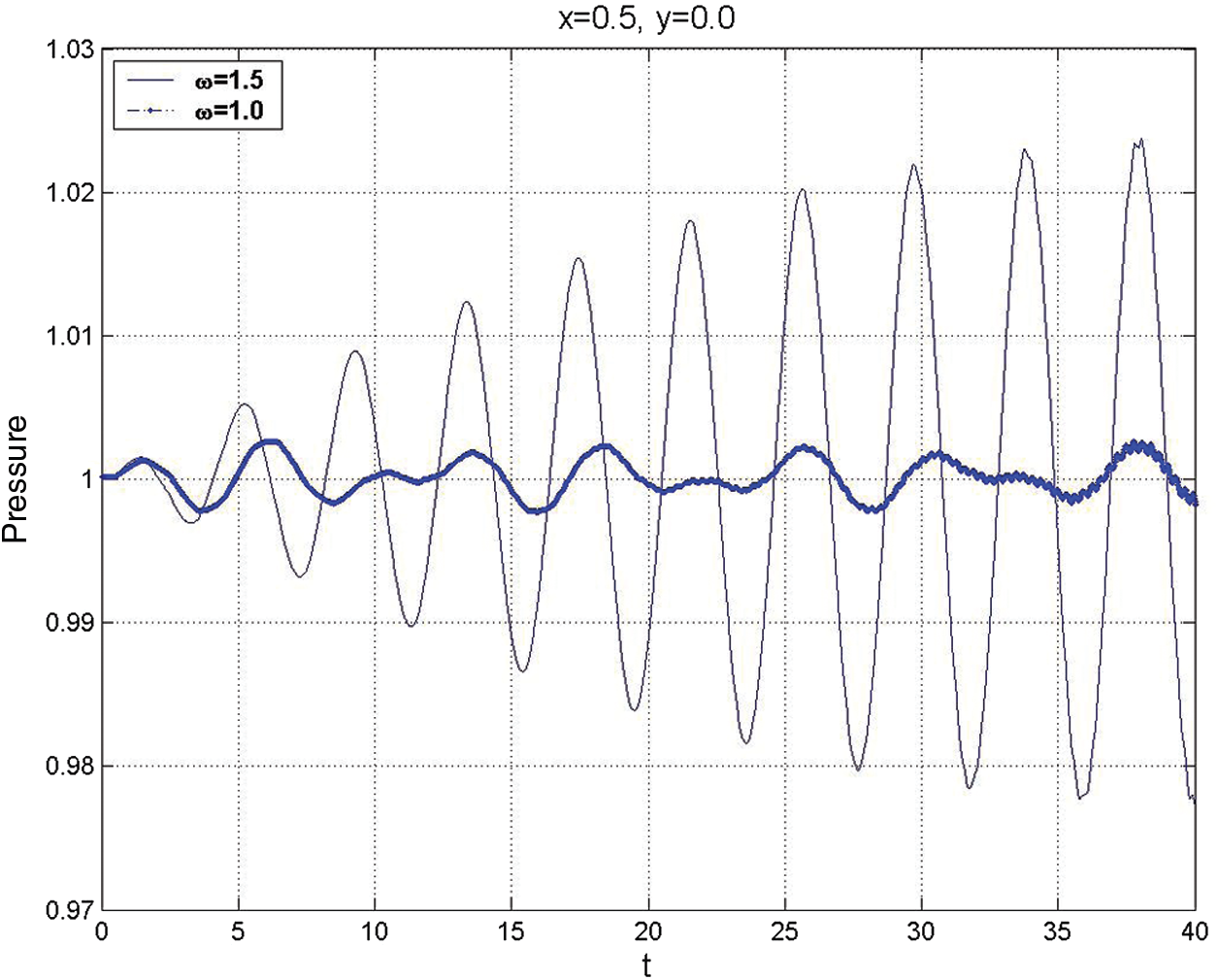
Figure 6: The pressure-time history at the mid-length of the chamber,
Lower and higher-order calculations are formulated to find a weakly nonlinear solution within the core flow, which defines the eigenfunctions’ acoustic damping time. The lowest order acoustic equations, valid for the limit
Our previous study [26] revealed that a weakly nonlinear theory is required to describe the acoustic evolution for a longer time. Thus, the perturbation analysis for higher-order calculations is used to find a weakly nonlinear solution within the core-flow to provide additional verification for the acoustic damping time of the eigenfunctions.
Moreover, the higher-order calculations revealed that the quadratic nonlinear convective terms could not be a source of intermodal energy transfer at the O(M2) approximation level. As a result, energy in eigenfunction modes cannot be damped by quadratic convection effects when “open box” eigenfunctions are the basis set for the Fourier series. At the same time, the O(M3) cubic nonlinearities are responsible for nonlinearization in the cavity of the SRM chamber. It follows that wave-wave interactions (non-harmonic behaviour of eigenfunction amplitudes) will occur over a time scale long compared to the acoustic time
Finally, we may conclude that Figs. 4 and 5 support the remarks above by comparing a finite-difference solution for the 2-D, nonlinear, unsteady parabolized Navier–Stokes equations and the one-dimension linear acoustic theory equations.
5.2 Acoustic Fluid Dynamics Interaction
The second category of the results is devoted to examining the unsteadiness of the rotational fluid flow that arises from the interaction between the longitudinal axial pressure waves and the steady injection from the side-wall. The first case of the second set is implemented for the rotational velocity and vorticity when t = 32 for
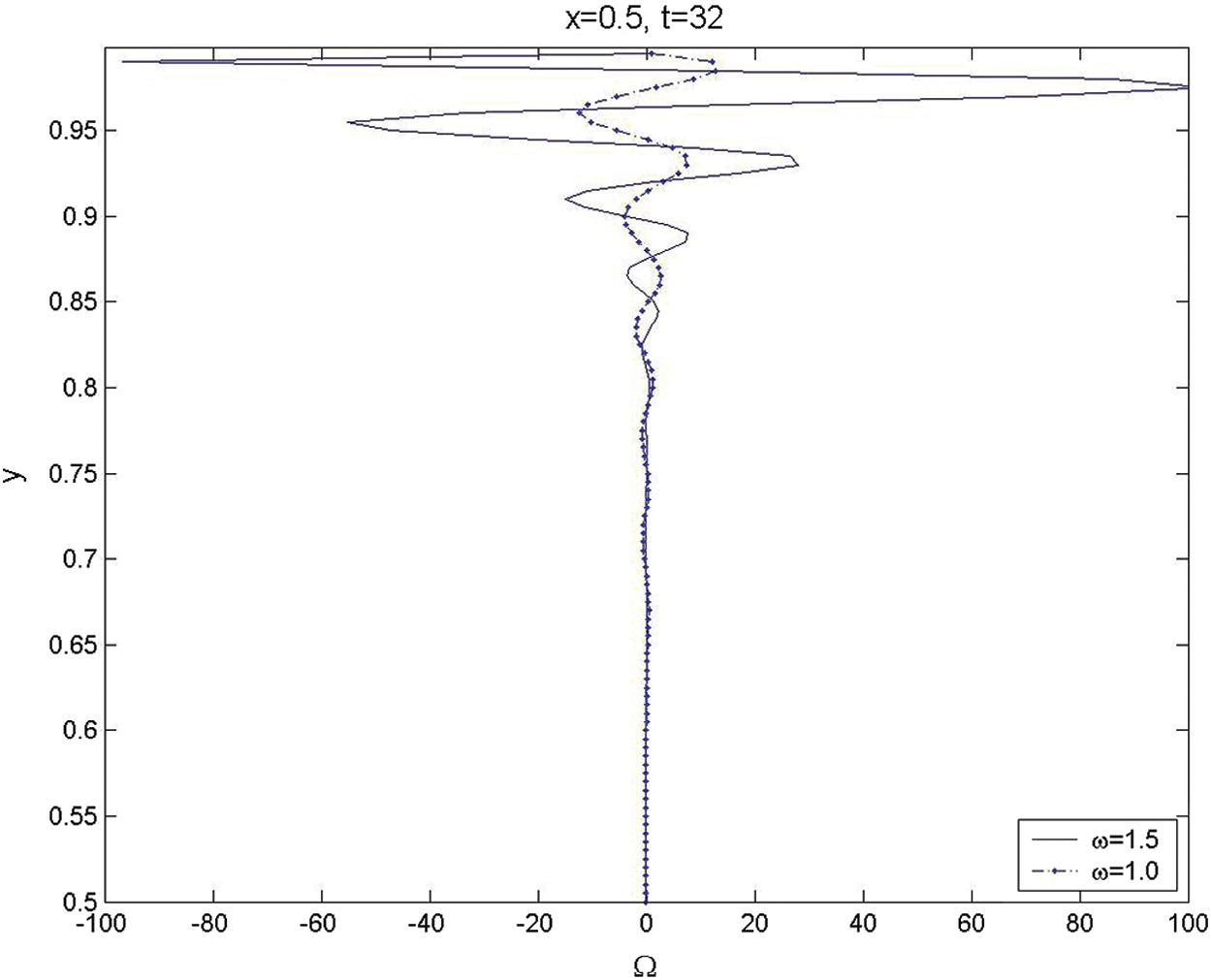
Figure 7: The transverse variations for unsteady vorticity across the chamber at
The results show that the rotational fluid flow is generated at the side-wall due to the interaction process and is then convected vertically toward the centerlines as time increases. It is found that the amplitude of the vorticity wave oscillations near the surface is generally larger than that away from the wall for both the non-resonance (
The effect of the injected Mach number on the generation and evolution of the unsteady vorticity is presented in Fig. 8 at t = 32 for
It is noticed that the amplitudes of the axial rotational velocity and the generated unsteady vorticity increase as the injected Mach number increases. Moreover, the vorticity front for M = 0.01 is located at y = 0.64, while for M = 0.02 is found to be at y = 0.4 from the centerline. This means that the vorticity field for the larger Mach numbers proceeds and fills faster than that for the smaller Mach numbers. Zhao et al. [19] predicted this trend, for the actual radial position as a function of the Mach number and time, as
The above derived front location in Eq. (87) is measured from the centerline. Fig. 9 shows that the analytical time-dependent vorticity front location (
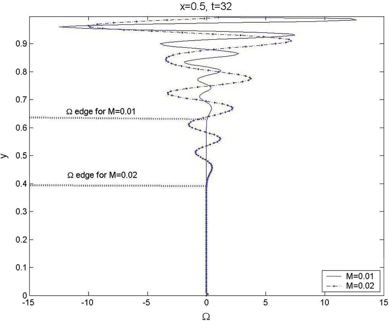
Figure 8: The transverse variations for unsteady vorticity across the chamber at x = 0.5, t = 32, and
The comparison between the analytical result for the vorticity front in Fig. 7 at t = 32, Mach number M = 0.01 and 0.02 with the numerical result locations in Fig. 8 show an excellent qualitative and quantitative agreement. Moreover, the vertical propagation of the generated vorticity front is found to be nearly linear as M = 0.01, and this tendency disappears as Mach number increases and the nonlinearity effect becomes predominant, as seen in Fig. 9.
The vorticity topography for
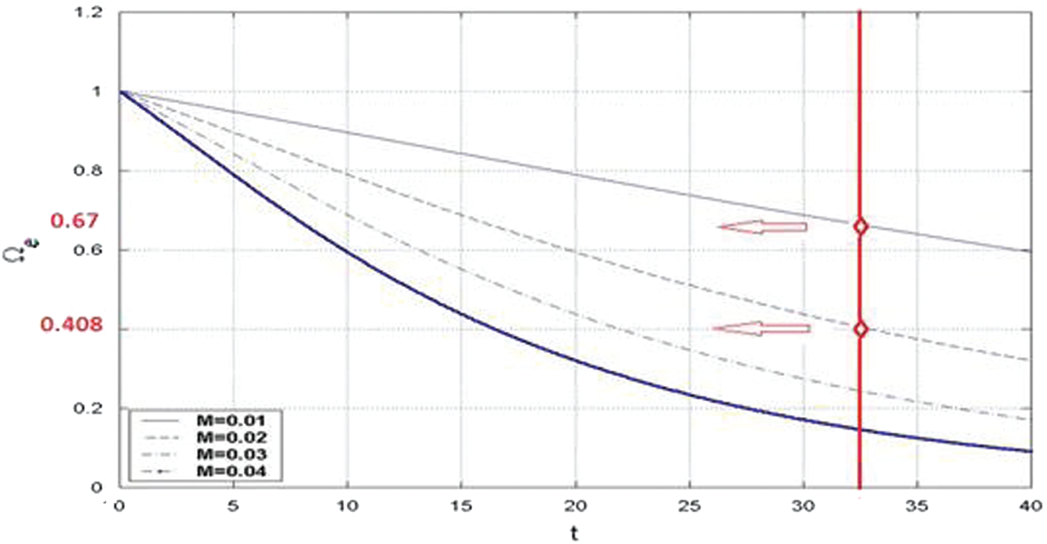
Figure 9: Analytical time-dependent vorticity front location (
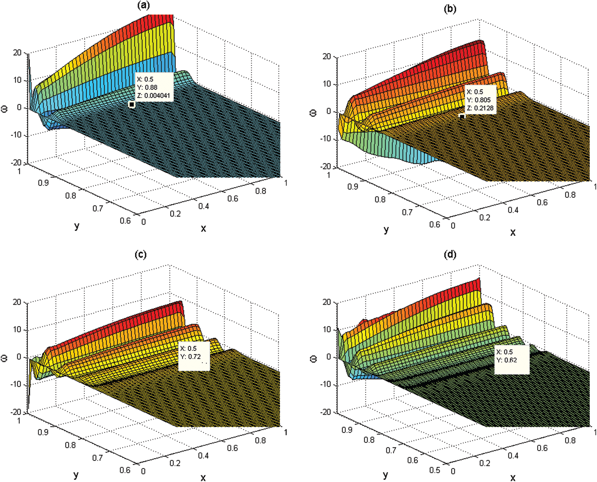
Figure 10: (a–d) Computational vorticity topographies that show the vorticity generation and penetration across the whole chamber at times
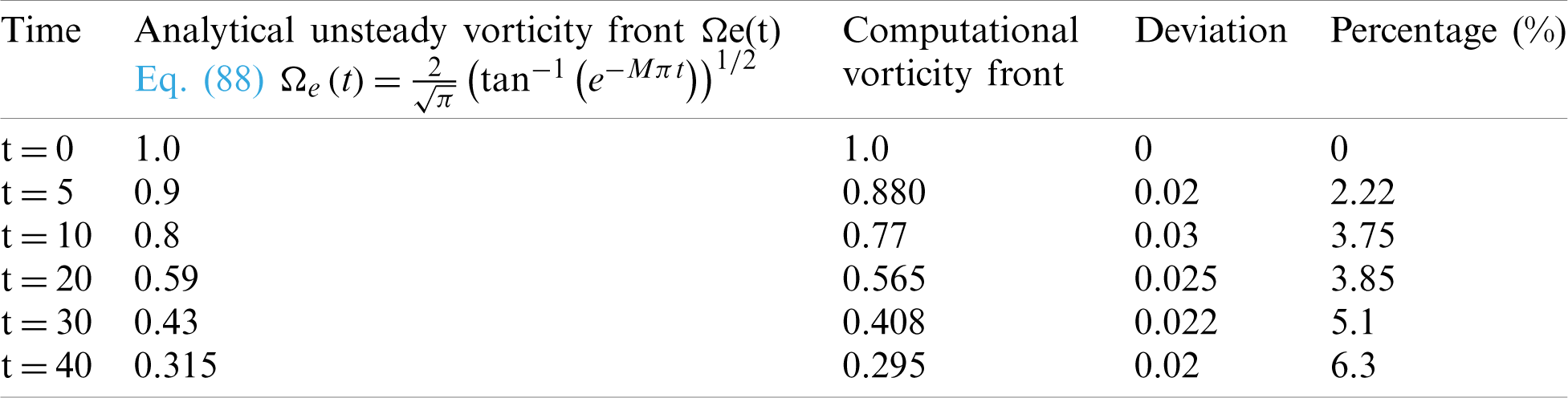
Table 1: Comparison between the analytical solution and the computational solution for the vorticity edge at
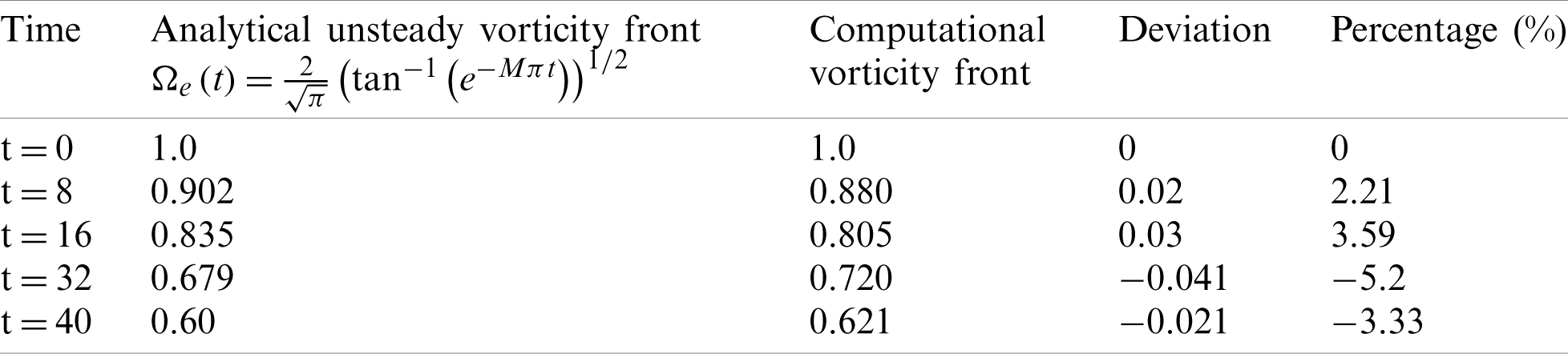
Here again, it is noted that the vorticity is generated at the sidewall and then penetrated and fill the entire chamber as time increase. Tab. 1 shows the locations of the vorticity fronts from the computational results presented in Figs. 10a–10d at t = 0, 8, 16, 32, and 40 and from the analytical solutions of Eq. (87). It is noted that deviations between the weakly nonlinear analytical solution and the computational solution are found to be O (10−2). This verification reveals that the numerical techniques with the treatment of the boundary conditions using NSCBC are suitable for solving the whole Navier–Stokes equations in similar chambers to the solid rocket.
To verify results for Mach number of 0.02, the transverse variations of rotational axial velocity (uv) at several different times mid-length in the chamber for
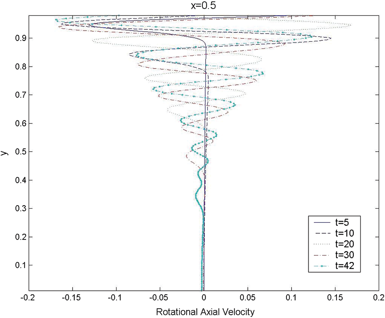
Figure 11: The transverse variations for rotational axial velocity across the chamber at
The results imply that the rotational field extends to cover nearly the entire chamber by t = 42. Moreover, the unsteady vorticity topography at two different times t = 20 and 40 for Re = 3 * 105,
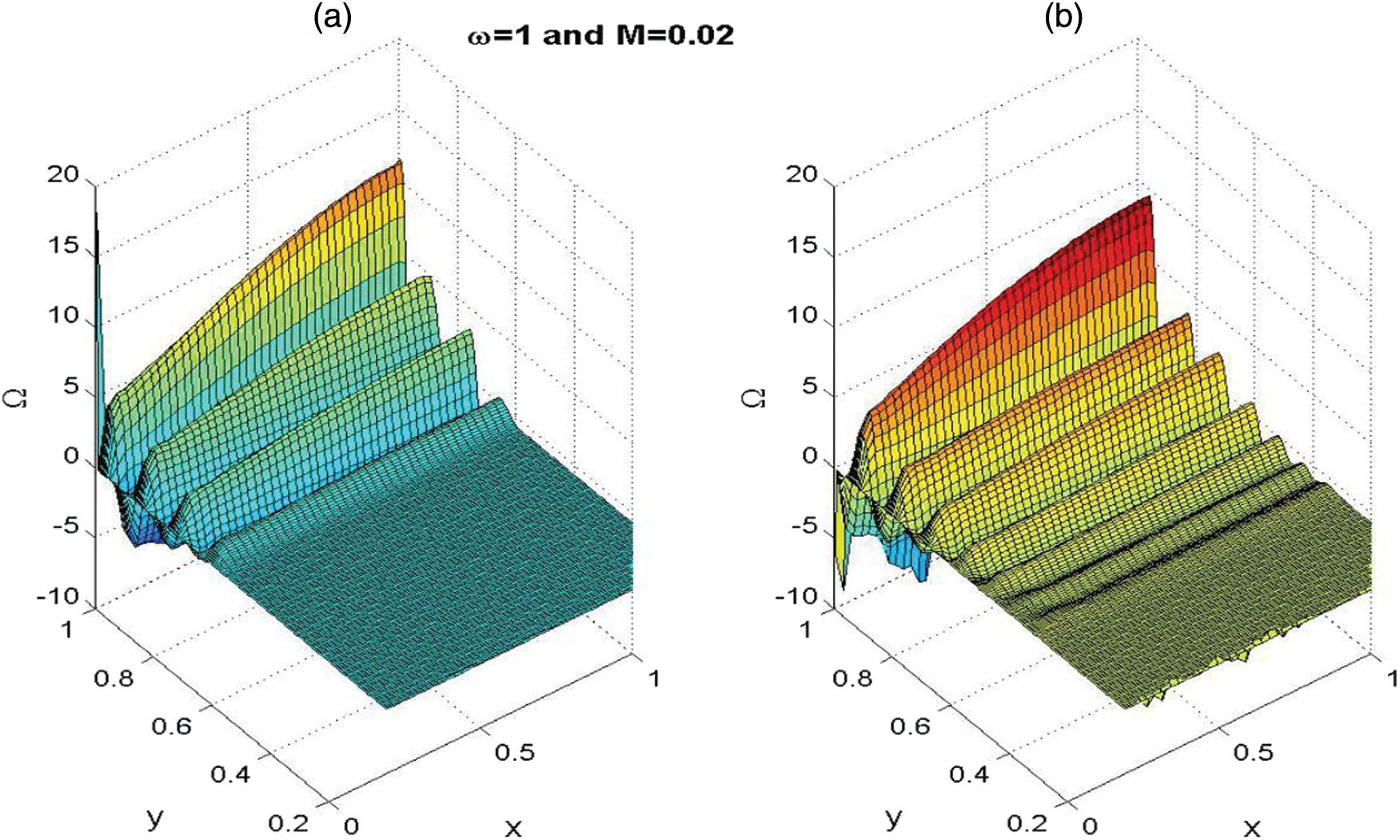
Figure 12: The vorticity topography for
From the results, it is noted that the absolute amplitude of the unsteady vorticity increases with increasing axial distance downstream. Moreover, the vorticity front moves almost parallel to the injection surface, and monotonic variation is noticed.
The last case study of the second set is for the generation and evolution of the temperature disturbance that accompanies the vorticity generation in the first case study. Fig. 13 shows the transverse temperature variations mid-length in the chamber for
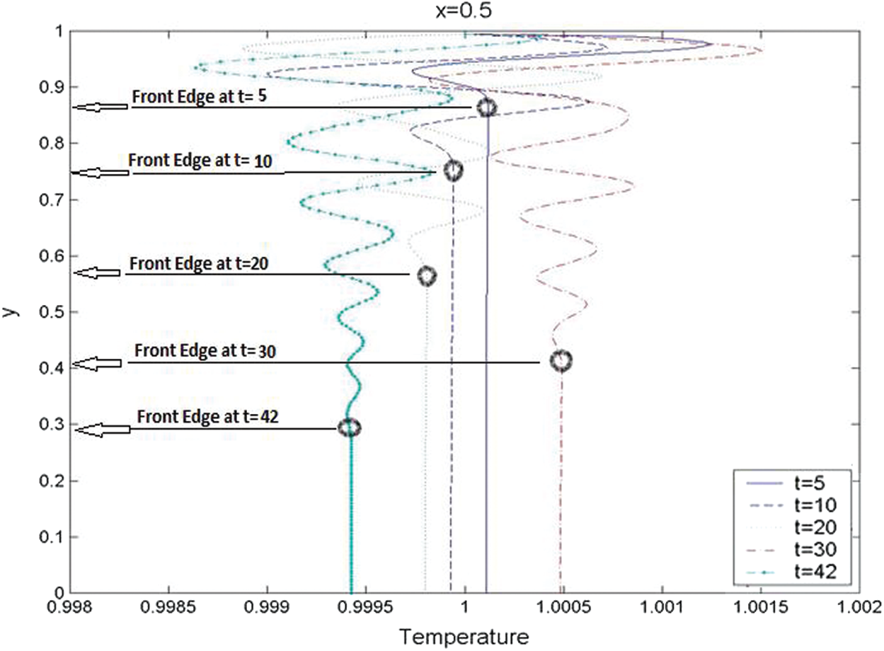
Figure 13: The transverse variations for the computational temperature variations across the chamber at
It is clearly noted that the fluctuation of the transverse temperature gradient at the injection surface is larger than that away from the injection surface. Here again, the variation can be attributed to a combination of oscillations at the forcing frequency and eigenfunction oscillations that exist for
Table 2: Comparison between the analytical solution and the computational solution for the vorticity edge at M = 0.02
An investigation to chamber flow turbulence modelling in a rectangular channel with a side-wall mass injection has been studied and validated in our previous study in [42,43]. We concluded that the RSM v2-f and SST k–
In the present paper, we only explain some important features of this flow configuration. Due to the continuous side-wall mass addition, the axial flow velocity increases towards the duct exit, and the flow is subjected to a strong streamline curvature, as shown in Fig. 14.
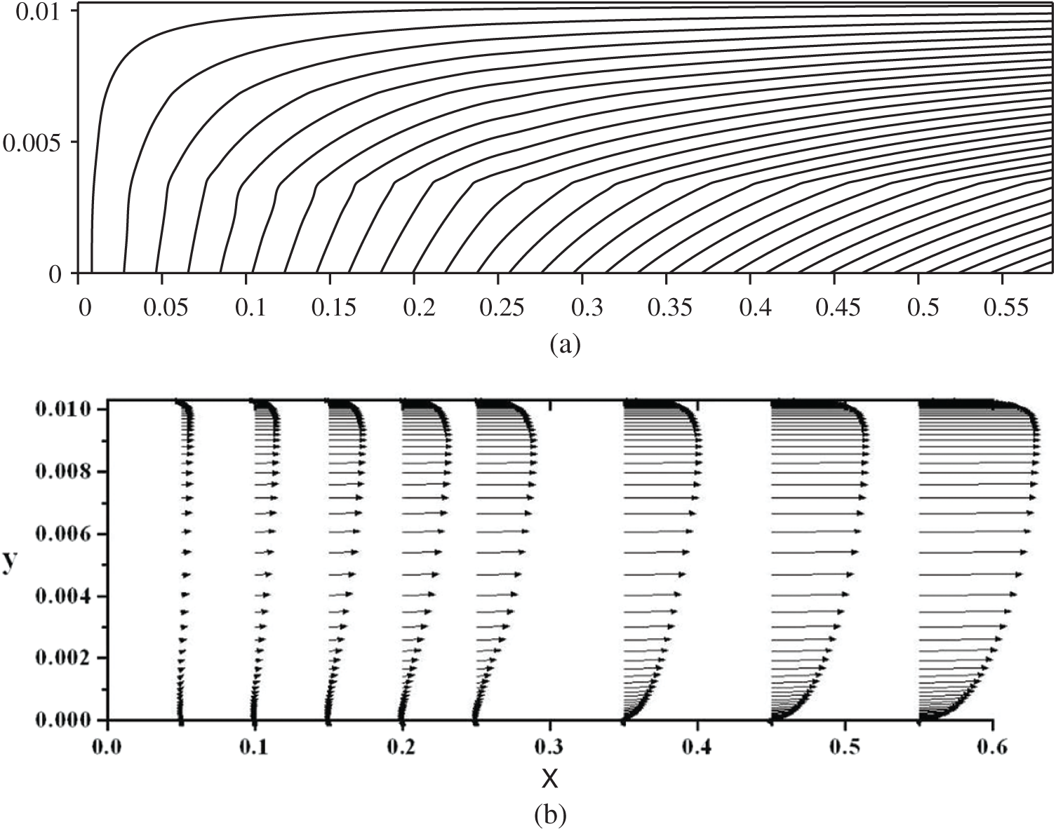
Figure 14: Streamlines and velocity vectors of the internal flow field in a simulated solid rocket motor chamber with side-wall injection
This velocity gradient and streamlined curvature results in an increase in turbulent kinetic energy production. As a result, the turbulent kinetic energy increases towards the duct exit, as shown in Fig. 15.
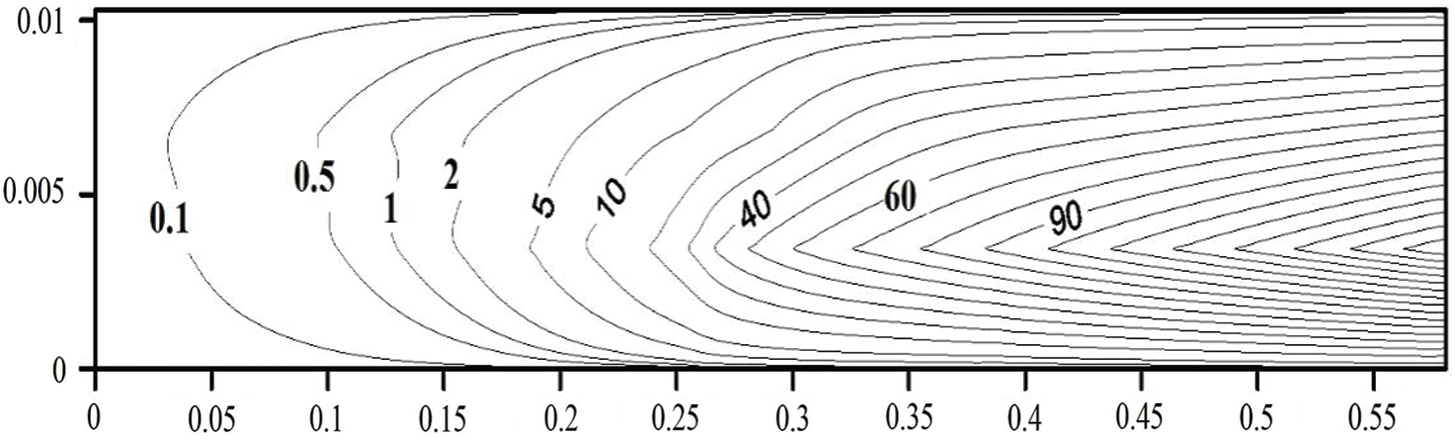
Figure 15: Contours of turbulent kinetic energy (m2/s2) in a simulated solid rocket motor chamber with side-wall injection
Therefore, the possibility of a laminar-to-turbulent transition exists. One way to identify the transition from laminar to turbulent is to examine the wall friction coefficient. Fig. 16 shows the friction coefficient obtained using different turbulent models. The friction coefficient, cf, is calculated as follows:
where
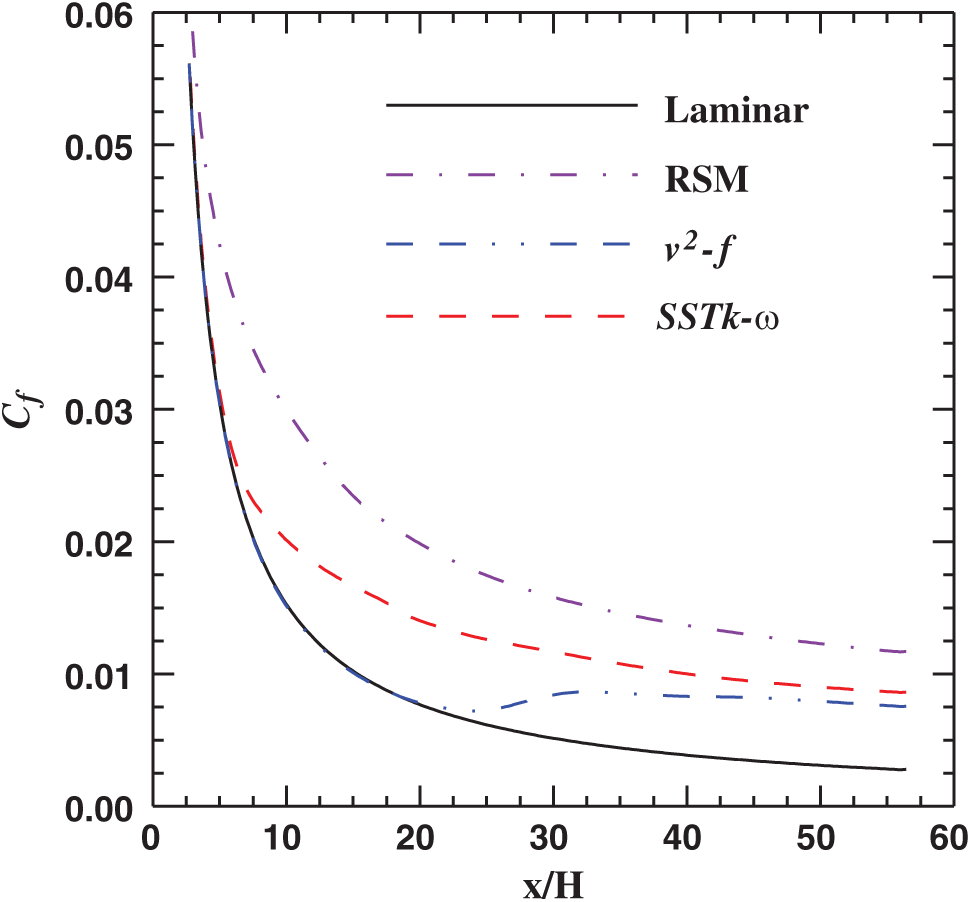
Figure 16: Distribution of the local friction coefficient along the wall of the solid rocket motor chamber with side-wall injection
The results shown reveal that the flow is laminar near the head end and transitions to turbulence at a certain axial distance. Dunlap et al. [45] and Griffond et al. [46] reported similar observations. Only the v2-f turbulence model can predict this phenomenon accurately. Therefore, the v2-f model is the appropriate choice for flow with a side-wall mass injection. Distribution of the local friction coefficient along the wall of the solid rocket motor chamber with side-wall injection is predicted. This comparison showed coupling between the generated unsteady vorticity arising from acoustics-fluid dynamics interaction and the turbulence intensity that exists strongly downstream of the rocket chamber.
Computational, analytical, and experimental approaches are integrated to study the complex wave patterns generated in a chamber with end-wall disturbances and the interactions with steady side-wall mass addition.
Results for the acoustic field show a bounded solution for the non-resonance frequency, while beats phenomena are observed near resonance frequency. A reasonable comparison between the experimental and computational approaches is seen.
The computational results for the rotational fields show that severe shear stresses may be generated beside the injection side-wall and transferred via convection over time to fill the entire chamber. The analytical and computational results show an excellent agreement for the propagation of the unsteady vorticity and its edges. It is seen that the amplitude of the generated shear stresses and the wavelength are many times larger beside the injection surface than near the centerline. These important phenomena reveal that the grid generation techniques must cluster near the centerline to capture the shorter wave cycles around the chamber centerline. By comparing the weakly nonlinear analytical solution and the computational solution for the vorticity front locations at different times and Mach numbers, the deviations between the two results were found to be O (10−2). This verification reveals that the numerical techniques with the treatment of the boundary conditions using NSCBC is suitable for solving the whole Navier–Stokes equations in chambers similar to the solid rocket chamber.
The effect of including turbulence models in predicting the internal flow characteristics is explained by a comparison between the laminar and turbulent simulation. The comparison showed coupling between the generated unsteady vorticity arising from acoustics-fluid dynamics interaction and the turbulence intensity that exists strongly downstream of the rocket chamber. Moreover, the importance of the turbulence studies with the aspect ratio of twenty suggests that the DNS may provide a better understanding for the impact of the transverse movement of the vorticity peak on the behaviour of the erosive burning.
In the context of propellant combustion, the intensive unsteady vorticity generation and the associated shear stresses can be anticipated to have a direct impact on the stability of burning real solid rocket propellant. Moreover, more intensive computations are required to account for the existence of the convergent–divergent nozzle along with the end-wall disturbances.
Acknowledgement: The authors wish to record their gratitude to DSR, King Abdulaziz University, for their technical and financial support. This research was funded by the Deanship of Scientific Research (DSR), King Abdulaziz University, Jeddah, Kingdom of Saudi Arabia, Grant No. 829-722-D1435.
Author Contributions: Conceptualization, A.H. and F.A.; methodology, F.A. and A.H.; software, A.H.; validation, A.H., F.A. and M.A.; formal analysis, F.A.; investigation, A.H. and F.A.; resources, A.H.; data curation, M.A.; writing–-original draft preparation, A.H.; writing–-review and editing, F.A and M.A.; visualization, A.H. and F.A.; project administration, M.A.; funding acquisition, F.A. and M.A. All authors have read and agreed to the published version of the manuscript.
Funding Statement: This research was funded by the Deanship of Scientific Research (DSR), King Abdulaziz University, Jeddah, Kingdom of Saudi Arabia, Grant No. 829-722-D1435.
Conflicts of Interest: The authors declare that they have no conflicts of interest to report regarding the present study.
1. Hegab, A. M., Jackson, T. L., Buckmaster, J., Stewart, D. S. (2001). Nonsteady burning of periodic sandwich propellants with complete coupling between the solid and gas phases. Journal of Combustion and Flame, 125(1–2), 1055–1070. DOI 10.1016/S0010-2180(01)00226-7. [Google Scholar] [CrossRef]
2. Kochevets, S., Buckmaster, J., Jackson, T. L., Hegab, A. (2001). Random packs and their use in modeling heterogeneous solid propellant combustion. Journal of Propulsion and Power, 17(4), 883–891. DOI 10.2514/2.58202001. [Google Scholar] [CrossRef]
3. Hegab, A. M., Sait, H. H., Hussain, A., Said, A. S. (2014). Numerical modeling for the combustion of simulated an SRM propellant. Computers & Fluids, 89(12), 29–37. DOI 10.1016/j.compfluid.2013.10.029. [Google Scholar] [CrossRef]
4. Zhao, Q., Kassoy, D. R. (1994). The generation and evolution of unsteady vorticity in a solid rocket engine chamber. Proceedings of the 32th Aerospace Sciences Meeting, Reno, Nevada, USA. pp. 779. [Google Scholar]
5. Kirkkopru, K., Kassoy, D. R., Zhao, Q., Staab, P. L. (2002). Acoustically generated unsteady vorticity field in a long narrow cylinder with sidewall injection. Journal of Engineering Mathematics, 42, 1(1), 65–90. DOI 10.1023/A:1014348029944. [Google Scholar] [CrossRef]
6. Staab, P. L., Zhao, Q., Kassoy, D. R., Kirkkopru, K. (1999). Coexisting acoustic-rotational flow in a cylinder with axisymmetric sidewall mass addition. Physics of Fluids, 11(10), 2935–2951. DOI 10.1063/1.870152. [Google Scholar] [CrossRef]
7. Erickson, R., Markopoulos, N., Zinn, B. (2001). Finite amplitude acoustic waves in variable area ducts. AIAA-01-1099, 39th AIAA Aerospace Sciences Meeting and Exhibit, Reno, NV, USA. [Google Scholar]
8. Zaripov, R. G., Ilhamov, M. A. (1976). Nonlinear gas oscillations in a pipe. Journal of Sound and Vibration, 46(2), 245–257. DOI 10.1016/0022-460X(76)90441-7. [Google Scholar] [CrossRef]
9. Merkli, P., Thomann, H. (1975). Thermoacoustic effects in a resonance tube. Journal of Fluid Mechanics, 70(1), 161–177. DOI 10.1017/S0022112075001954. [Google Scholar] [CrossRef]
10. Wang, M., Kassoy, D. R. (1995). Nonlinear oscillation in a resonant gas column: An initial-boundary value study. SIAM Journal on Applied Mathematics, 55, 4(4), 923–951. DOI 10.1137/S003613999324290X. [Google Scholar] [CrossRef]
11. Jimenez, J. (1973). Nonlinear gas oscillations in pipes. Part 1. Theory. Journal of Fluid Mechanics, 59(1), 23–46. DOI 10.1017/S0022112073001400. [Google Scholar] [CrossRef]
12. Sileem, A. A. (1998). Nonlinear evolution of resonant acoustic oscillations in a tube ended with variable area portion. International Conference on Energy Research & Development, Kuwait. [Google Scholar]
13. Sileem, A. A., Nasr, M. (2003). An experimental study on finite amplitude oscillations in ducts: The effect of adding variable area part to the open end of constant-area resonant tube. Alexandria Engineering Journal, 42(4), 397–409. [Google Scholar]
14. Seymour, B. R., Mortell, M. P. (1973). Resonant acoustic oscillation with damping: Small rate theory. Journal of Fluid Mechanics, 58(2), 353–373. DOI 10.1017/S0022112073002636. [Google Scholar] [CrossRef]
15. Disselhorst, J. H. M., Wijngaarden, L. V. (1980). Flow in the exit of open pipes during acoustic resonance. Journal of Fluid Mechanics, 99(2), 293–319. DOI 10.1017/S0022112080000626. [Google Scholar] [CrossRef]
16. Garcia-schafer, J. E., Linan, A. (2001). Longitudinal acoustic instabilities in slender solid propellant rockets: Linear analysis. Journal of Fluid Mechanics, 437, 229–254. DOI 10.1017/S0022112001004323. [Google Scholar] [CrossRef]
17. Staab, P. L., Zhao, Q., Kassoy, D. R., Kirkkopru, K. (1999). Co-existing acoustic-rotational flow in a cylinder with axisymmetric sidewall mass addition. Physics of Fluids, 11(10), 2935–2951. DOI 10.1063/1.870152. [Google Scholar] [CrossRef]
18. Rempe, M., Staab, P. L., Kassoy, D. R. (2000). Thermal response for an internal flow in a cylinder with time-dependent sidewall mass addition. AIAA 2000-0996, 38th Aerospace Science Meeting, Reno, NV, USA. [Google Scholar]
19. Zhao, Q., Staab, P. L., Kassoy, D. R., Kirkkopru, K. (2000). Acoustically generated vorticity in an internal flow. Journal of Fluid Mechanics, 13, 247–285. DOI 10.1017/S0022112000008454. [Google Scholar] [CrossRef]
20. Flandro, A. (1995). Effect of vorticity on rocket combustion stability. Journal of Propulsion and Power, 11(4), 607–625. DOI 10.2514/3.23887. [Google Scholar] [CrossRef]
21. Xuan, L. J., Majdalani, J. A. (2018). Point-value enhanced finite volume method based on delta function approximations. Journal of Computational Physics, 355(2), 37–58. DOI 10.1016/j.jcp.2017.10.059. [Google Scholar] [CrossRef]
22. Vuillot, F., Avalon, G. (1991). Acoustic boundary layers in solid propellant rocket motors using Navier-Stokes equations. Journal of Propulsion and Power, 7(1), 231–239. DOI 10.2514/3.23316. [Google Scholar] [CrossRef]
23. Smith, T. M., Roach, R. L., Flandro, G. A. (1993). Numerical study of the unsteady flow in a simulated solid rocket modtor. 31th Aerospace Science Meeting, Reno, NV, USA. [Google Scholar]
24. Tseng, C. F., Tseng, I. S. (1994). Interaction between acoustic waves and premixed flames in porous chamber. AIAA 94-3328, 32th Aerospace Science Meeting, Reno, NV, USA. [Google Scholar]
25. Chu, W. W., Yang, V., Majdalani, J. (2003). Premixed flame response to acoustic waves in a porous-walled chamber with surface mass injection. Combustion and Flame, 133(3), 359–370. DOI 10.1016/S0010-2180(03)00018-X. [Google Scholar] [CrossRef]
26. Vetel, J., Plourde, F., Kim, S. D., Guery, J. F. (2003). Numerical simulations of wall and shear layer instabilities in a cold flow set-up. Journal of Propulsion and Power, 19(2), 297–306. DOI 10.2514/2.6111. [Google Scholar] [CrossRef]
27. Vetel, J., Plourde, F., Kim, S. D. (2004). Amplification of a shear-layer instability by vorticity generation at an injecting wall. AIAA Journal, 42(1), 35–46. DOI 10.2514/1.9028. [Google Scholar] [CrossRef]
28. Hegab, A. M. (1998). A study of acoustic phenomena in solid rocket engines (Ph.D. Thesis). Menoufia University, Egypt, (Carried out at the University of Colorado at Boulder). [Google Scholar]
29. Hegab, A. M., Kassoy, D. R., Sileem, A. A. (1998). Numerical investigation of acoustic-fluid dynamics interaction in an SRM chamber/nozzle model. AIAA Paper 98-0712, 36th Aerospace Science Meeting. Reno, NV, USA. [Google Scholar]
30. Liou, T. M., Lien, W. Y. (1995). Numerical simulations of injection driven flow in a two-dimensional nozzleless solid rocket motor. Journal of Propulsion and Power, 11, 4(4), 600–606. DOI 10.2514/3.23886. [Google Scholar] [CrossRef]
31. Beddini, R. A. (1986). Injection-induced flows in porous-walled ducts. AIAA Journal, 24(11), 1765–1773. DOI 10.2514/3.9522. [Google Scholar] [CrossRef]
32. Yamada, K., Goto, M., Ishikawa, N. (1976). Simulative study on the erosive burning of solid rocket motors. AIAA Journal, 14(9), 1170–1175. DOI 10.2514/3.61451. [Google Scholar] [CrossRef]
33. Sabnis, J. S., Gibeling, H. J., McDonald, H. (1989). Navier–Stokes analysis of solid propellant rocket motor internal flows. Journal of Propulsion and Power, 5(6), 637–664. DOI 10.2514/3.23203. [Google Scholar] [CrossRef]
34. Hegab, A. M., Wilson, S. A., El-Askary, W. A., El-Behery, S. M., Yousif, K. A. (2001). Mathematical modeling of reactive fluid flow in solid rocket motor combustion chamber with/without nozzle. International Conference on Aerospace Sciences and Aviation Technology, Vol. 5, pp. 24–26. Military Technical College, Cairo, Egypt. [Google Scholar]
35. Hegab, A. M., Nasr, M. (2008). Unsteady vorticity fields in a long narrow channel with end wall disturbances and sidewall injection. Proceedings of ICFDP9, Ninth International Congress of Fluid Dynamics & Propulsion, Alexandria, Egypt. [Google Scholar]
36. Kirkkopru, K., Kassoy, D. R., Zhao, Q. (1996). Unsteady vorticity generation and evaluation in a model of solid rocket motor. Journal of Propulsion and Power, 12(4), 646–654. DOI 10.2514/3.24085. [Google Scholar] [CrossRef]
37. MacCormack, R. W. (1982). A numerical method for solving the equations of compressible viscous flow. AIAA Journal, 20(9), 1275–1281. DOI 10.2514/3.51188. [Google Scholar] [CrossRef]
38. Gottlieb, D., Turkel, E. (1976). Dissipative two-four methods for time-dependent problems. Mathematics of Computation, 30(136), 703–723. DOI 10.1090/S0025-5718-1976-0443362-6. [Google Scholar] [CrossRef]
39. Hegab, A. M., Sait, H. H., Hussain, A. (2014). Impact of the surface morphology on the combustion of simulated solid rocket motor. Mathematical Problems in Engineering, 2015(2), 485302–485311. DOI 10.1155/2015/485302. [Google Scholar] [CrossRef]
40. Hinze, J. O. (1975). Turbulence. New York: McGraw-Hill Publishing Co. [Google Scholar]
41. Versteeg, H. K., Malalasekera, W. (2007). An introduction to computational fluid dynamics: the finite volume method. London: Pearson Education. [Google Scholar]
42. Balabel, A., Hegab, A. M., Nasr, M., El-Behery, S. M. (2011). Assessment of turbulence modeling for gas flow in two-dimensional convergent–divergent rocket nozzle. Applied Mathematical Modelling, 35(7), 3408–3422. DOI 10.1016/j.apm.2011.01.013. [Google Scholar] [CrossRef]
43. El-Askary, W. A., Balabel, A., El-Behery, S. M., Hegab, A. (2011). Computations of a compressible turbulent flow in a rocket motor-chamber configuration with symmetric and asymmetric injection. Computer Modeling in Engineering & Sciences, 82(1), 29–54. DOI 10.32604/cmes.2011.082.029. [Google Scholar] [CrossRef]
44. Avalon, G., Casalis, G., Griffond, J. (1998). Flow instability and acoustic resonance of channels with wall injection. 34th AIAA/ASME/SAE/ASEE Joint Propulsion Conference and Exhibit. Cleve-land, OH, USA. [Google Scholar]
45. Dunlap, R., Blackner, A. M., Waugh, R. C., Brown, R. S., Willoughby, P. G. (1990). Internal flow field studies in a simulated cylindrical port rocket chamber. Journal of Propulsion and Power, 6(6), 690–704. DOI 10.2514/3.23274. [Google Scholar] [CrossRef]
46. Griffond, J., Casalis, G., Pineau, J. P. (2000). Spatial instability of flow in a semi-infinite cylinder with fluid injection through its porous walls. European Journal of Mechanics-B/Fluids, 19(1), 69–87. DOI 10.1016/S0997-7546(00)00105-9. [Google Scholar] [CrossRef]
 | This work is licensed under a Creative Commons Attribution 4.0 International License, which permits unrestricted use, distribution, and reproduction in any medium, provided the original work is properly cited. |