Computer Modeling in Engineering & Sciences

DOI: 10.32604/cmes.2021.015913

ARTICLE

Discrete Element Modelling of Dynamic Behaviour of Rockfills for Resisting High Speed Projectile Penetration

Tingting Zhao1, Y. T. Feng2,*, Jie Zhang1, Zhihua Wang1 and Zhiyong Wang1

1College of Mechanical and Vehical Engineering, Taiyuan University of Technology, Taiyuan, 030024, China
2Zienkiewicz Centre for Computational Engineering, Swansea University, Swansea, SA2 8PP, UK
*Corresponding Author: Y. T. Feng. Email: y.feng@swansea.ac.uk
Received: 26 January 2021; Accepted: 04 March 2021

1  Introduction

In the protection engineering, rockfills have advantages of high strength, easy access and low cost which make them ideal protection materials to resist the penetration. A series of experimental studies on anti-penetration capabilities of various bursting layers consist of soil, rock or concrete, and bursting layers with different configurations are carried out by many scientific research groups [1–5]. The influence of configurations and contents of protection layers on the deflection of projectiles has been investigated which indicates that the yaw-inducing techniques are very effective for projectiles with a large ratio of length to diameter and the projectiles would be damaged by unsymmetrical impact force to some extents. Langheim et al. [2] carried out a series of penetration experiments with rockfill and concluded that good protection capability can be achieved by selecting proper size, gradation and compaction density of rockfill.

For the numerical simulation of rockfill protection problems, commercial software such as AUTODYN, LS-DYNA and ABAQUS are widely used. Mu et al. [6] conducted simulations of the rockfill target and concluded that a good protective capacity could be achieved when the size, thickness and strength of the rockfill target were matched with the projectile. Fang et al. [7] studied the penetration process of rockfill layers considering the random distribution of particle size and shape. In the study of penetration behavior of the reinforced concrete by Zhang et al. [8,9], the influence of size and fraction of coarse aggregates on the trajectory stability were considered using the meso-scale model.

As a rockfill system is inherently discrete and discontinuous, the Discrete Element Method (DEM) [10] can be used to simulate the interaction between rock particles and the projectile directly and obtain the energy dissipation, penetration depth and projectile velocity. Furthermore, the internal mechanism of macroscopic response can be revealed from the microscopic level. At present, the study of DEM modelling on dynamic behavior of the rock particle system under impact load is rare, and the traditional DEM with spherical elements is mostly adopted in some penetration problems [11,12]. The fundamental different behaviour of a spherical particle from a polyhedral particle makes the use of spheres to model rockfill systems less reliable.

The difficulty of using polyhedron as a basic discrete element lies in modelling of the contact behaviour between polyhedral particles. In this work, a newly developed Minkowski difference-based contact modelling methodology in [13,14] for convex polyhedral particles will be adopted to model the dynamic behaviour of rockfill systems under projectile impact. In this methodology, the contact overlap between two polyhedra is taken to be their Minkowski difference distance, or simply the Minkowski overlap [14]. The collision detection to establish if two polyhedra are in contact or not is called the GJK algorithm [15]. The actual Minkowski overlap of two contacting polyhedra is obtained by the Expending Polytope Algorithm (EPA) [16]. The contact force is computed based on a linear normal contact model. Using the Minkowski overlap and related contact features in the normal model ensures that the total elastic energy will be conserved for convex polyhedra in an elastic impact, which leads to robust discrete element simulations of complex problems including rockfill systems.

The paper is organised as follows. The next section will briefly introduce all the aspects of a polyhedral DEM model based on the methodology developed in [13,14], including the definition of Minkowski overlap and related contact features, the procedures to compute the features and the contact models used. Section 3 describes the quaternion based orientation representation of polyhedra and a symplectic time integration scheme to solve the angular motion of polyhedral particles. Numerical simulations of a rockfill system are conducted in Section 4 where a rock particle generation scheme is described first, followed by the description of all the model and parameters used for the simulations. Effects of the system parameters on the dynamic behaviour of the rockfill system subject to a high speed projectile impact are presented and discussed. Some conclusions are drawn in Section 5.

2  Convex Polyhedral Discrete Element Model

Consider two convex polyhedral particles in contact. Each polyhedron can have any number of vertices and flat faces. Each face is a convex polygon which can also have any number of vertices/edges. The discrete element modelling of the contact between these two polyhedra should establish if they are in contact, and if so then completely defines the contact features, including contact overlap (or volume), normal direction, contact point and contact force. This section will briefly describe the relevant definitions, computational procedures and contact models used for polyhedra in the current work, which are collectively called the polyhedral DEM model. The description below is mainly adopted from [13,14] where more details can be found.

Note that the polyhedral DEM model presented below is equally applicable to convex polygons. For simplicity, convex polygons will be used for all illustrations.

2.1 Minkowski Contact Features

Let A and B be the two polyhedra concerned. The Minkowski difference of A and B, denoted as A⊖B, is defined by

A⊖B={a-b:a∈A,b∈B}(1)

The boundary of A⊖B is denoted as ∂(A⊖B). It is easy to establish that A and B is in contact or not is equivalent to that the origin is inside or outside A⊖B. Fig. 1 shows three contact states of a quadrilateral (A) and a triangle (B) together with the corresponding Minkowski differences in relation to the origin.

Figure 1: The Minkowski differences of a quadrilateral A and a triangle B, with B at three vertical position, and their contact states (a) separation, (b) touch, (c) overlap

When A and B are in contact, or the origin is inside A⊖B, the contact (vector) distance between A and B is defined as the minimum distance dM that can be applied to B such that A and B are just in touch:

dM=argminv∈ℝn{∥v∥:v∈∂(A⊖B)}(2)

Then the contact overlap, denoted as δM, is the magnitude of dM, and is termed as the Minkowski overlap in [14], while the unit vector of dM defines the contact normal nM, i.e.,

dM=δMnM,∥nM∥=1

The point c on ∂(A⊖B) that has the shortest distance dM to the origin o is called the contact point on A⊖B. The two corresponding points of c on the boundaries of A and B are respectively c1 and c2, and they are called the contact points on A and B, respectively. A common contact point cM for both A and B can be taken as

cM=(c1+c2)/2(3)

Here, δM, nM, c, c1, c2 and cM are called the Minkowski contact features in [14], and they are illustrated in Fig. 2. Different contact types that are classified in [13] include vertex-edge, edge-edge for both polygons and polyhedra, and vertex-face and edge-face, face-face for polyhedra.

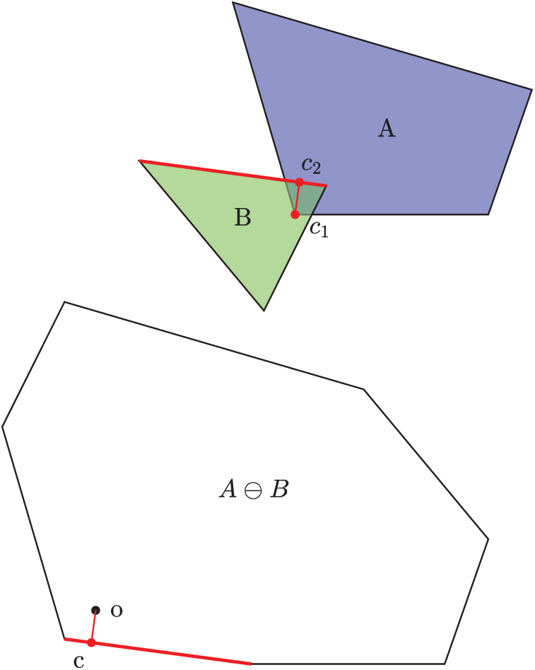
Figure 2: The contact features between A and B: contact point c on A⊖B, contact points c1 and c2 on A and B respectively; oc defines both dM and the contact normal nM and is perpendicular to ∂(A⊖B). The contact type is vertex-edge

2.2 Contact Detection and Evaluation of Contact Features

The whole contact detection procedure in DEM includes three steps: Global search, local resolution and contact force calculation. In the first step, particles concerned, regardless of their actual shapes, are approximated by a simple enclosure (a bounding sphere or box). The objective of the global search is to establish a potential contact list for each particle. In the second step, the contact between two particles in the contact list is further checked based on their actual geometric shapes to establish the real contact state: separation, or overlap. For a pair of particles which are in contact, their contact forces will be evaluated in the third step.

As many effective global search algorithms already exist, there will be no further discussion about the global search. The third force evaluation step will be described in the next subsection. This subsection will focus on the local contact resolution for two polyhedra. The computational procedures required to fulfil the objective are to effectively determine if two polyhedra are in contact or not, and if so to obtain the Minkowski contact features defined in the preceding subsection.

Determining if two convex polyhedra are in contact or not is conducted by GJK [15], while computing the Minkowski contact features is achieved by EPA [16] in the current work. Both algorithms are very effective and their details are also described in [13]. The two initial issues associated with EPA for some special contact cases mentioned in [13] are resolved in [14].

2.3 Contact Force Models

After the Minkowski contact features of two polyhedra, mainly including overlap δM, normal n and contact point cM, are obtained by EPA, the normal contact force Fn can be evaluated as

Fn=fn(δM)nM(4)

where the function fn defines the magnitude of the force. As suggested in [14], fn can have a general power-law form

fn=knδMn(5)

where kn is the stiffness coefficient, and n≥1 is the exponent. A linear spring contact model is recovered when n = 1, while a “Hertz-type” contact model is obtained when n = 3/2. Although the contact model (4) seems to be the same as other overlap based contact models commonly used in DEM, the crucial difference for non-spherical particles is that in the current model both the overlap and the contact normal, together with the contact point where Fn is applied, are the Minkowski contact features defined in a particular manner as described in Section 2.1. As formally proved in [14], using the Minkowski contact features in (4) for convex particles ensures that elastic energy will be conserved in any contact scenarios for an elastic impact. This is another energy-conserving normal contact model developed within the framework of the general contact theory established in [17], and is an alternative to the contact volume based contact models developed in [18] based on the same contact theory.

The tangential contact will be modelled by the classic Coulomb friction law. No detail needs to be described.

3  Rotational Motion of Polyhedral Particles

When all contact forces are evaluated for a particle, the dynamic governing equation for the translational motion of the particle can be expressed as

mu¨+cu̇+Fc=Fa(6)

where m is the mass of the particle; c is the coefficient of viscous damping; Fc is the resultant contact force from all the contacts concerned; Fa is the summation of all other applied forces on the particle; and u̇ and u¨ are the velocity and acceleration of the particle. The equation can be numerically solved used the standard central difference or leapfrog time integration scheme. No detail will be offered here.

It is the angular motion of non-spherical particles that imposes significant challenges to discrete element modelling. Based on Newton’s second law, the governing equation for the rotational motion of a particle can be written as

d(Jω)dt=p(7)

where J and ω are the moment inertia tensor and angular velocity vector of the particle respectively, and p represents the resultant moment/torque acting on the particle. An explicit damping term is omitted here, but can be included in p. Note that J, ω and p are in the global coordinate system, and in particular J is a function of time for non-spherical shapes. (7) can be expended into a form

Jω̇+ω×Jω=p(8)

This is clearly a highly non-linear second order differential equation, and imposes some challenges to obtain its numerical solution accurately and effectively.

For a given non-spherical particle in general, its three principal moments of inertia are assumed available and denoted by a 3×3 diagonal matrix J̄=diag{J̄1,J̄2,J̄3}, and the corresponding three principal moment axes at the current time are denoted as a 3×3 matrix Rt in the global coordinate system. These three directions form a local coordinate system attached to the particle, with the mass centre of the particle as the origin. J is related to J̄ by

J=RtJ̄RtT(9)

As Rt is a function of time when the particle rotates, so is J. In the local coordinate system, (7) is reduced to the so-called Euler’s equation

J¯ω¯.+ω¯×J¯ω¯=p¯(10)

where ω̄={ω̄1,ω̄2,ω̄3}=RtTω is the local angular velocity and p̄={p̄1,p̄2,p̄3}=RtTq is the local moment.

As J̄ is a diagonal matrix, (10) can be decoupled into component form

J¯iω¯˙i+(J¯k−J¯j)ω¯jω¯k=p¯i (11)

where (i,j,k) is one of three permutations of (1,2,3):{1,2,3},{2,3,1},{3,1,2}. These decoupled equations can be numerically solved. Nevertheless, how to represent and update the orientation of the particle dictates the efficient and accuracy of solving the rotational motion of a non-spherical particle in DEM.

3.1 Orientation Representation of Polyhedral Particles

Unlike the centrally symmetric spherical particle, representing the orientation of a polyhedral particle is critical to the polyhedral DEM model for the determination of rotational motion and contact detection. In this work, the orientation of a polyhedron is represented by a quaternion which provides the most effective way to handle 3D rotation of a non-spherical shape.

A quaternion q consists of one real component and three imaginary components and can be expressed by a four-element vector with one scalar plus a vector: q=(w,v). Geometrically a quaternion corresponds to a rotation state in space. In this work q is assumed to be a unit quaternion:

∥q∥2=w2+v⋅v=1(12)

A quaternion can be alternatively denoted in the following form which represents a rotation around a unit axis (vector) n by an angle θ:

q(θ,n)=(cosθ2,sinθ2n)(13)

The inverse or conjugate of a quaternion q is simply

q-1=(w,-v)=(cosθ2,- sinθ2n)(14)

which geometrically represents a rotation around the same axis n with the same angle θ but in the opposite direction. Also (q-1)-1=q.

Two rotations can be combined into one using quaternion multiplication. The multiplication of two quaternions q1=(w1,v1) and q2=(w2,v2) is defined as

q2q1=(w1w2-v1⋅v2,w2v1+w1v2+v2×v1)(15)

which is equal to applying the rotation q1 first and followed by the rotation q2. Quaternion multiplication is not commutative because the vector cross product n2×n1 is not commutative.

A quaternion can be applied to rotate a vector. The rotation of a vector v by a quaternion q is denoted as R(q,v) and defined by

R(q,v)=qvwq-1(16)

where vw=(0,v) is the quaternion extension of the vector v. The rotated vector assumes to take only the imaginary part of the quaternion R(q,v).

Similarly, define an inverse rotation operator R-1(q,v) as

R-1(q,v)=R(q-1,v)=q-1vwq(17)

3.2 Numerical Time Integration of Angular Motion Using Quaternion

The time integration scheme presented below is based on [19], which is one of symplectic integers that possess some superb long term conservation properties and therefore are widely used in general non-linear dynamics.

Consider a discretised time interval [tn,tn+1] with the time step Δt=tn+1-tn. Assume that at time t = tn, ω=ωn and the orientation quaternion q=qn are obtained, and the total applied moment p=pn is given and remains constant in the interval. The task is to numerically solve Eq. (7) to obtain ω=ωn+1 and q=qn+1 at time t = tn+1.

First an intermediate angular moment L is computed by

L=R(qn,J̄R(qn-1,ωn))+Δtpn(18)

and then is transformed to the local coordinate system

L̄={L̄1,L̄2,L̄3}=R(qn-1,L)(19)

In order to obtain the orientation qn+1, a series of incremental rotations around the three axes are required to be performed. Define an (incremental) quaternion associated with the (local) angular moment L̄, the (local) moment inertia J̄, a local rotation axis i=(1,2,3) and the time step Δt as

qit(L̄,J̄,Δt)={(cs,si,0,0),i=1(cs,0,si,0),i=2(cs,0,0,si),i=3(20)

where

si=ϕi1+ϕi2/4;cs=1-ϕi2/41+ϕi2/4;withϕi=0.5ΔtL̄i/J̄i(21)

Further define an updated quaternion qu of a given quaternion q in terms of L̄, J̄, Δt and a direction i as

qiu(q,L̄,J̄,Δt)=qR(qi-t(L̄,J̄,Δt),L̄)(22)

Now the orientation qn+1 can be obtained from qn by applying five consecutive incremental rotations as

qn1=q1u(qn,L̄,J̄,0.5Δt);qn2=q2u(qn1,L̄,J̄,0.5Δt)qn3=q3u(qn2,L̄,J̄,Δt);qn4=q2u(qn3,L̄,J̄,0.5Δt)qn+1=q1u(qn4,L̄,J̄,0.5Δt)(23)

Finally the global angular velocity ωn+1 can be updated as

ωn+1=R(qn+1,ω̄n+1)(24)

where ω̄n+1 is the local angular velocity which can be computed as

ω̄n+1=J̄-1L̄={L̄1/J̄1,L̄2/J̄2,L̄3/J̄3}(25)

4  Numerical Simulation of a Rockfill System

4.1 Generation of the Rockfill Sample

The polyhedral DEM outlined in the previous sections has the advantage of modelling irregular convex polyhedral particles directly. A rockfill system consisting of polyhedral rock particles is generated through the three-dimensional Voronoi meso model [8]. A graded rockfill sample can be obtained by introducing random parameters for shape and size control.

Firstly, N seeds are randomly placed into a given region V. Then the region is divided into N cells using the Voronoi tessellation technique, following the principle that the distance of arbitrary point within the polyhedron from its corresponding seed Si is less than the distance from any other seed. A vertex P of the polyhedron satisfies the following equation:

Vi=⋂i≠j{P∈D∣d(P,Si)≤d(P,Sj),i≠j}(26)

in which

d(P,S)=(Px-Sx)2+(Py-Sy)2+(Pz-Sz)2(27)

The region volume V, the number of cells N and the average effective radius of cells r (i.e., the average distance between two seeds) have the following relation:

N=V(4π/3)r3(28)

The initial 3D Voronoi diagram is shown in Fig. 3, in which each cell is a convex polyhedron that can be considered as a rockfill particle. The seamless cells need to be shrunk to obtain the scattered rocks. The shrinking factor of vertices within one cell must be the same to keep the convexity of the polyhedron. The shrinking factors for different cells are determined according to the actual grade of the rockfill sample. The shrinking factor for polyhedra with the size in the range [di,di+1] is obtained by

q[di,di+1]=1-di+1dmax+ωdi+1-didmax(29)

where dmax is the maximum diameter, and ω is a random number between 0 and 1. The vectors from the vertices of each cell to the corresponding seed need to be shorten by this shrinking factor.

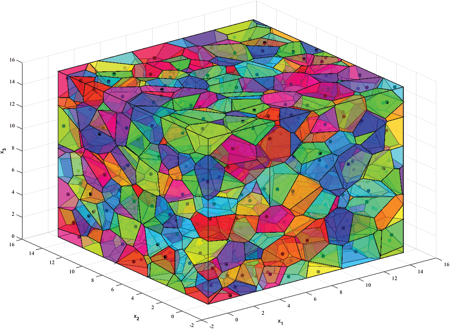
Figure 3: Initial 3D Voronoi diagram

The vertices and connectivities of the polyhedra obtained from the above procedure are imported to our polyhedral DEM procedure. However, the polyhedral sample generated by the Voronoi technique is very loose as shown in Fig. 4. To obtain a condense rockfill target, all rockfills drop under gravity and then are compressed by moving the top wall boundary downwards until a desired packing configuration is achieved.

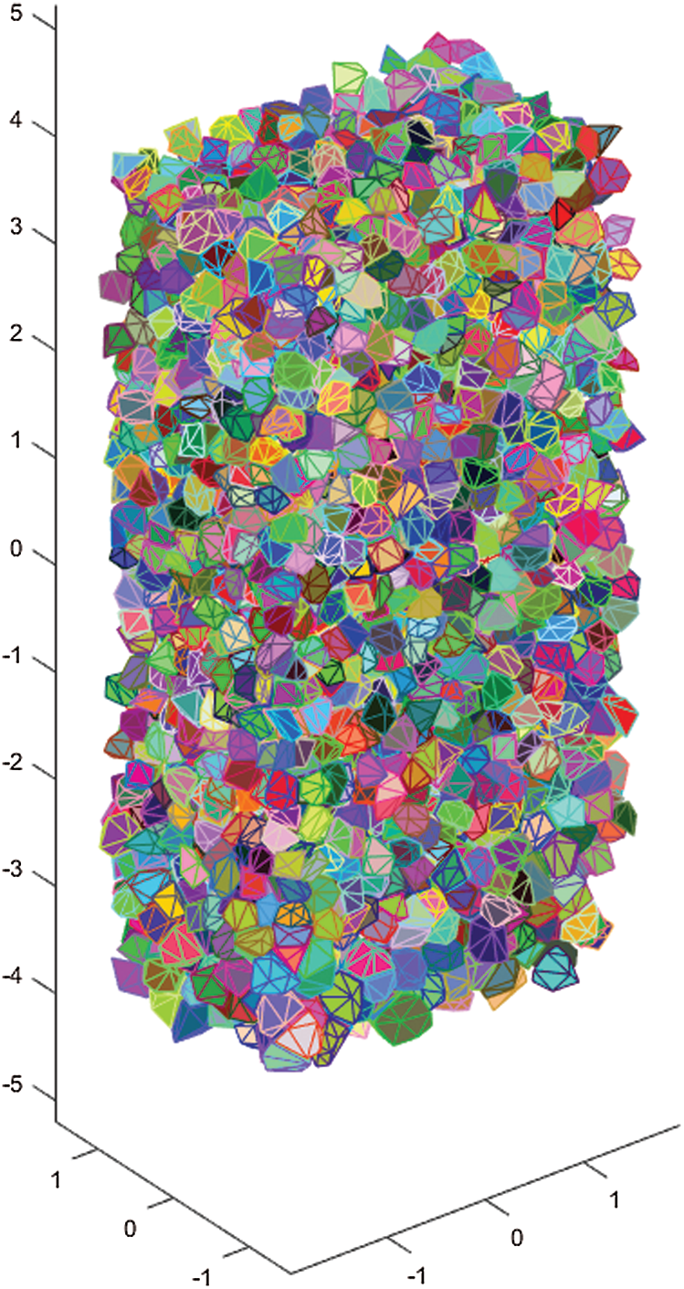
Figure 4: Loose rockfill sample generated by Voronoi technique

4.2 Penetration Simulation

The projectile penetrating the rockfill layer of a composite structure target is simulated using the above polyhedral DEM. The projectile is an axi-symmetric object with its cross-section profile shown in Fig. 5, with H=800 mm, R=500 mm and D=150 mm. The inner cavity of the projectile is not shown here but its effects on the mass and moments of inertia are properly considered. The projectile is also discretised into a polyhedron using the profile geometric parameters where 12 divisions are applied to the head part and 36 divisions are used in the circumference around the axis, so it can also be modelled by the same polyhedral DEM procedure. The composite structure target is not considered. The rockfill layer has the dimensions of 3.5m (L)×2.7m (W)×3.5m (H).

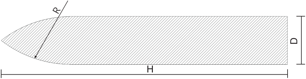
Figure 5: Profile of the projectile

The penetration model of the rockfill layer is generated by the method described in Section 4.1 and displayed in Fig. 6 with the projectile. The projectile strikes the rockfill layer from the centre of the left face at around 0.5 ms with an initial velocity of 1200 m/s and completely penetrates through the layer at around 3.5 ms.

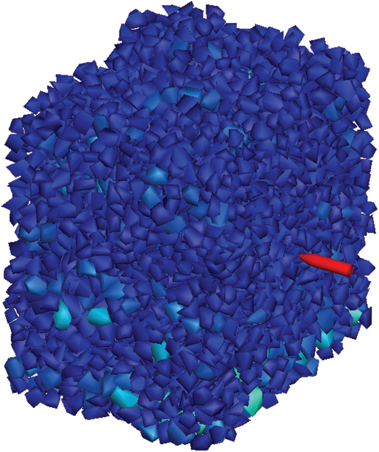
Figure 6: Penetration model of the rockfill layer

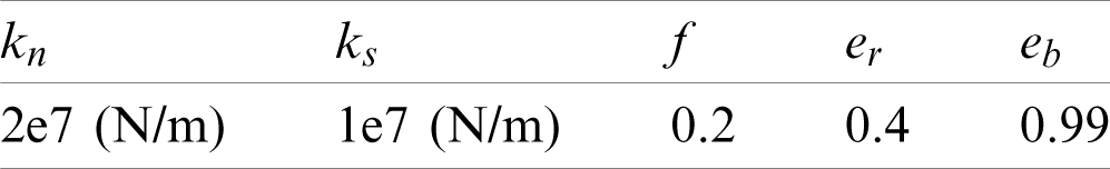
A number of microscopic parameters need to be selected to describe the contact behaviour between the rock particles and also between the particles and the projectile. These include the normal stiffness kn of the linear normal contact model, the tangential stiffness ks, the coefficient of friction f and the coefficient of restitution e. The sensitive analysis of the parameters shows that the stiffnesses and the coefficient of friction have a minor influence on the penetration results, while the coefficient of restitution affects the final results significantly.

The velocity of the projectile decreases rapidly which cannot penetrate the rockfill layer when a small restitution is selected between the projectile and the particles. It is difficult to measure the trajectory and penetration resistance of the projectile in the field experiment. Therefore, the microscopic parameters cannot be determined precisely by adjusting the values to make the simulation results consistent with the experimental results. At the current stage, the main purpose of the penetration simulating is to show the potential benefit of modelling the interaction between the projectile and the rockfill using the polyhedral DEM. The values for all the parameters are selected as shown in Tab. 1, where er and eb are the coefficient of restitution between the rock particles and between the particles and the projectile respectively. With these parameters, the residual velocity of the projectile is almost the same as the experimental results.

Table 1: Microscopic parameters of DEM model

A series of penetration simulations has been conducted using the above polyhedral DEM model and microscopic parameters. The mean size of rockfill particles is selected as 100, 130, 175, 200, 290 mm, respectively. The particle size obeys a normal distribution within the range of ±10% of the mean size. The interaction between the projectile and the rockfill particles is visualised by the DEM simulation. The profile at the ZY plane of the penetration process for the 100 mm sample is shown in Fig. 7. It clearly shows that the affected range by the projectile is about 6–7 times of the average rock size with the target position at the centre.

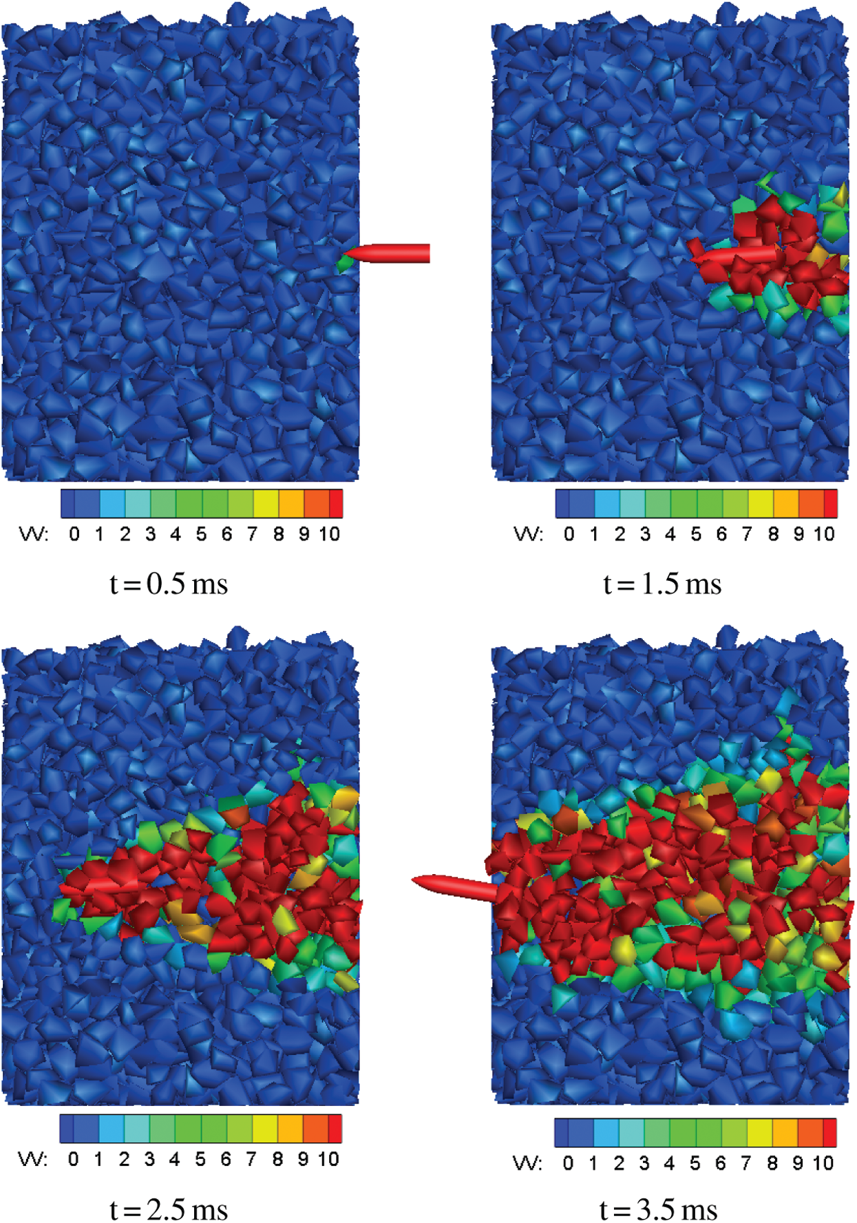
Figure 7: Configurations of the penetration process at the four time instants for the 100 mm rockfill sample

The residual velocity, the penetration resistance and the deflection angle curves are shown in Fig. 8. The five residual velocity curves locate in two regions. For the four curves of the rockfill size between 100 to 200 mm, the residual velocity is from 1000 to 1025 m/s. The residual velocity of the 290 mm rockfill target is much larger than others as 1100 m/s. As the diameter of the projectile is around 150 mm, we can deduce that the target whose rockfill size is closer to the projectile diameter has a better velocity reduction effect. For the penetration resistance, the fluctuation range of the sample with the large size rockfill is larger than that of the sample with the small size rockfill (100 and 130 mm). It is because the resistance is the resultant force of all the rockfill acting on the projectile, the number of rockfill contacted with the projectile is more stable for the target with a small size rockfill. The curves of the deflection angle show a similar tendency with the curves of the residual velocity. The deflection angle for all the targets stays in the range from 10∘ to 20∘. As expected, the target with 290 mm rockfill has a very large deflection angle.

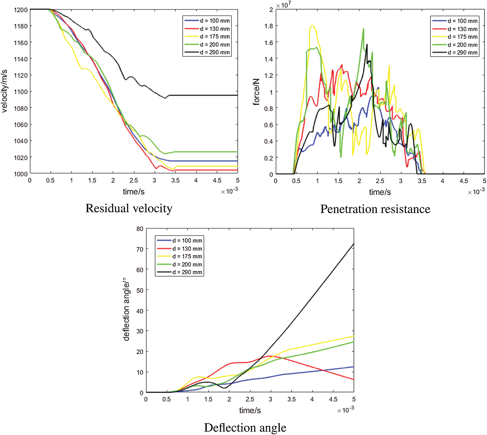
Figure 8: Simulation results for rockfill targets with different particle size

5  Conclusion

This paper has presented a polyhedral DEM method for modelling the dynamic behaviour of rockfills for resisting high speed projectile penetration. The key issues of the polyhedral DEM method have been systematically introduced including the calculation of the contact force and rotational motion of polyhedral particles. To determine the contact force, the contact relation of two convex polyhedra is conducted by GJK and then the Minkowski contact features are computed by EPA. This normal contact model is energy-conserving for any contact scenario of an elastic impact. To calculate the rotational motion, the orientation of polyhedral particles is expressed by a quaternion and the time integration is based on a symplectic splitting method. This polyhedral DEM method has been applied to model the dynamic behaviour of a rockfill system. The rockfill sample is generated by a three-dimensional Voronoi meso model with a specific particle size distribution. The penetrating process of a high speed projectile striking a rockfill target has been simulated. Some process variables of the projectile such as the residual velocity, penetration resistance, and deflection angle is monitored which can reflect the influence of the characteristics of the rockfill target on its anti-penetration performance. It can be concluded that the developed polyhedral DEM method is a potentially powerful numerical approach in analysing the dynamic behaviour of rockfill systems.

Acknowledgement: The authors wish to express their appreciation to the reviewers for their helpful suggestions which greatly improved the presentation of this paper.

Funding Statement: This work is partially supported by National Natural Science Foundation of China under Grant No. 12072217 and by Open Fund of State Key Laboratory of Coal Resources and Safe Mining, China University of Mining and Technology, Beijing, China [Grant No. SKLCRSM19KFA12]. The support is gratefully acknowledged.

Conflicts of Interest: The authors declare that they have no conflicts of interest to report regarding the present study.

This work is licensed under a Creative Commons Attribution 4.0 International License, which permits unrestricted use, distribution, and reproduction in any medium, provided the original work is properly cited.