Computer Modeling in Engineering & Sciences

DOI: 10.32604/cmes.2021.014662

ARTICLE

Method for Collision Avoidance in Spacecraft Rendezvous Problems with Space Objects in a Phasing Orbit

Danhe Chen*,1, A. A. Baranov2, Chuangge Wang1, M. O. Karatunov3 and N. Yu. Makarov3

1Nanjing University of Science and Technology, Nanjing, 210094, China
2Keldysh Institute of Applied Mathematics, Russian Academy of Sciences, Moscow, Russia
3Peoples’ Friendship University of Russia (RUDN University), Moscow, Russia
*Corresponding Author: Danhe Chen. Email: juliachen@njust.edu.cn
Received: 18 October 2020; Accepted: 13 January 2021

1  Introduction

Currently, Spacecraft rendezvous has been considered as one of the key technologies for on-orbit service, including space debris removing, on-orbit assembly, spacecraft repairing, and on-orbit refueling [1–3]. Several on-orbit service missions have been carried out as technology demonstration for a cooperative spacecraft, XSS of Air Force Research Laboratory [4], Demonstration for Autonomous Rendezvous Technology (DART) program of NASA [5], ETS-VII project of JAXA [6] and etc. Meanwhile, several satellite systems consisting of hundreds of objects are created. For each satellite system, it is necessary to solve the problem of its transfer to a given position, and as the significantly increasing number of space debris objects, the task to ensure flight safety appears. Due to the importance of the collision avoidance, numerous papers are devoted to solve the problem of possible collision between spacecraft with space debris(SD). Research on rendezvous techniques for non-cooperative targets is also conducted, in the vast majority of these work, the fact of a possible collision is determined. A much smaller research focus on the calculation methods of the avoidance maneuvers of spacecraft. In [7], model predictive control strategy is used to realize the docking of rotating targets in space.

Also, sliding mode control is widely used in spacecraft rendezvous considering the collision avoidance. Kasaeian et al. [8] utilized a robust guidance algorithm based on sliding mode method for a chaser to rendezvous with a target in space. Meanwhile, the terminal sliding mode control method is applied to tracking control problem for autonomous underwater vehicles (AUVs) [9,10], and a fixed-time terminal sliding mode control strategy introduced to produce an artificial gravity environment by spinning tether system in high eccentricity transfer orbit [11]; an adaptive fuzzy sliding mode control is proposed to solve the problem of spacecraft attitude tracking for space debris removal [12]. A novel sliding mode control strategy is developed to avoid entering dangerous areas during the implementation of the rendezvous procedure [13], and new neural sliding mode guidance is studies for maneuvering target in [14].

Considering the optimal problem of fuel consumption, Cao et al. [15] proposed an optimal artificial potential function sliding mode control with obstacle avoidance in mind, which effectively reduced fuel consumption. Similarly, model predictive control has been extensively applied to spacecraft rendezvous under various constraints, including obstacle constraints, velocity constraints. The control problem of spacecraft autonomous rendezvous in an elliptical orbit is studied in reference [16]. Christopher Jewison et al. used model predictive control to compute an optimal control strategy for a chaser attempting to rendezvous with obstacle avoidance constraints and in which obstacles are approximated to ellipsoids [17]. The computational load of model predictive control is enormous, but the on-board computational capacity is limited. A real-time nonlinear model predictive control (MPC) toolbox named MATMPC is utilized to solve this problem in work [18]. Impulse and continuous thrust are the most recommended maneuvers [19], under the constant thrust model, Qi et al. [20] designed a new constant thrust switch control law for the active collision avoidance maneuver of the chiller along a specific trajectory.

Since the calculation of special single impulse maneuver which thrust the protected spacecraft out of the dangerous area is quite simple, the main attention in these work is paid to determining the size of the dangerous area in which could be a collision [21,22]. Thus, this group of researches can be attributed to the first class study, in which the possibility of a collision is determined. This is due to the fact that in most of the work, whenever possible, a collision in one way or another uses the size of the protected area, and special avoidance maneuvers are considered in a relatively lack of research.

The difference of this work is that it does not consider special avoidance maneuvers, but seeks such a solution to the rendezvous problem in order to evade a possible collision in a phasing orbit if a danger exists. The second difference is that the hazardous area (the position of which are considered known, since that they can be determined by the algorithms given in the above papers) is considered not in the traditional coordinate space, but on the plane of the components of the eccentricity vector. In addition, the proposed method to solve the problem makes it easy to calculate rendezvous maneuvers that provide avoidance from several collisions or from “slow” collisions in a phasing orbit, when the protected spacecraft and the SD object fly dangerously close to each other for a long time.

The need seeking for such a solution to the rendezvous problem can be explained by several reasons. For example, at the spacecraft “Soyuz” and “Progress”, after performing the first two maneuvers (in 2–3 orbits) from a series of four connected maneuvers with a two-day rendezvous scheme, beginning from deaf turns where it is impossible to conduct maneuvers. If the phasing orbit formed by the first two maneuvers is dangerous in terms of collision with SD objects on it, then changing it with a special velocity and thereby avoiding the collision is no longer possible. Considering that, the only way out for solving this problem can be described as follows: firstly, the orbit after applied the first two impulses should be predicted under the optimal scheme, if in this orbit there is a possibility of a collision with SD, constraints should be added to find a solution to the rendezvous that the spacecraft will not pass through the danger zone after the first two impulses.

Moreover, even if it is predicted that no collision will occur, recalculation for rendezvous maneuvers in order to form a safe phasing orbit allows to reduce both the number of maneuvers performed and the total fuel costs.

The paper is organized as follows: In Section 2, mathematical description of the problem to be solved is introduced. The specific methodology and solution is presented in Section 3, which provide the optimal solutions in plane of eccentricity vector in different maneuvers. Conclusions are summarized in the end of the paper.

2  Mathematical Description of the Problem

Assume that the chasing spacecraft and the target spacecraft are located in close near-circular orbits (or the target spacecraft as a given point in the final orbit to which the chasing spacecraft should be transferred during the formation of satellite systems or groups). Then we can use the linearized equations to calculate the parameters of maneuvers, influence of earth’s non-spherical perturbation and atmospheric drag on the spacecraft here are not considered, and instant change in spacecraft velocity is assumed. Using the famous iterative method [23], the solution of the problem that satisfies the terminal condition of a given precision with all disturbance factors considered can be obtained. The motion equation of flight reaches a given target orbit as a result of N velocity impulses can be written in the following dimensionless form:

∑i=1N(ΔVri sinφi+2ΔVti cosφi)=Δex(1)

∑i=1N(-ΔVri cosφi+2ΔVti sinφi)=Δey(2)

∑i=1N2ΔVti=Δa(3)

∑i=1N(2ΔVri(1- cosφi)+ΔVti(-3φi+4sinφi))=Δt(4)

∑i=1N-ΔVzi sinφi=Δz(5)

∑i=1NΔVzi cosφi=ΔVz(6)

where Δex = efcosωf-e0cosω0, Δey = efsinωf-e0sinω0, Δa = (af − a0)/r0, Δt =λ0(tf − t0), Δz = z0/r0, ΔVz = Vz0/V0, ΔVri=ΔVri*/V0, Δ Vti=ΔVti*/V0, Δ Vzi=ΔVzi*/V0.

Here, “f”, “0” are the index indicating the final and initial orbits; ef, e0 are the eccentricities of the final orbit and initial orbit; af, a0 are the semi-major axis of orbits; ωf, ω0–angles between the direction to pericenter of the corresponding orbit and the direction to the point specified in the final orbit (the axis Ox is directed to this point); tf is the time required to reach the target point, t0 is the time, when spacecraft moving in initial orbit, the projection of radius vector on the plane of final orbit passing through the given point; z0 is the deviation distance between the initial orbit and the final orbit plane of the spacecraft at time t0; Vz0 is the lateral relative velocity at this moment; V0, λ0 are orbital velocity and angular velocity of motion along the circular orbit of radius r0 (r0 = af); N is the number of speed pulses; ϕi is the angle of application of the i-th impulse, measured from the given point in direction of the spacecraft motion; ΔVri*, ΔVti*, ΔVzi* are the radial, transversal, and lateral velocities of the i-th impulses, respectively. It must be taken into account that the angles ϕi are negative, since it was assumed that at the given point ϕf= 0 (this in particular explained the “ −” sign in Eq. (5)).

A multi-turn flight scheme is also assumed in this paper. This scheme has several advantages as shown below: Firstly, when the total characteristic velocity (TCV) of the rendezvous problem is equal to the TCV of the solution to transition problem (there is no restriction on flight time.), in this case a fairly wide range of the initial phase can be considered (phase is the difference in the latitude argument Δu). Secondly, after the first maneuvering interval, parameters of the formed orbit can be determined, and then after recalculation, the accuracy of second velocity impulse will be improved. Maneuvering intervals F1,…,FN, at which impulses can be applied, are usually given by the orbit number and the argument of latitude from the beginning to the end interval. Therefore, following restrictions on the applied angles of impulses are expressed as:

φ1∈F1φN∈FN(7)

where F1, …, FN are the given maneuvering intervals.

For ensuring rendezvous problems of spacecraft by maneuvers, it is necessary to determine the parameters of impulses ΔVri, ΔVti, ΔVzi, ϕi (i=1,…,N), at which the total TCV V is minimal:

ΔV=∑i=1NΔVi=∑i=1NΔVri2+ΔVti2+ΔVzi2(8)

Under the constraints defined by Eqs. (1), (6) and (7).

In this process, the protected area ranges are also determined. Since the rendezvous problem is solved and it is impossible to avoid collisions by changing position along the orbit, the minimum required deviation along the radius Δr is defined.

Here it is advisable to choose a four-impulses scheme to solve this problem, two impulses are applied at the first maneuvering interval, and two impulses are applied at the second maneuvering interval. The proposed approach is described in detail in the following section.

3  Results and Discussion Methodology

The magnitude of semi-major axis of the phasing orbit, which should be formed by the impulses of the first maneuvering interval, is uniquely determined from Eq. (4) (determined by the initial phase difference Δu). And the multi-turn flight allows an approximate estimation of the sum of transversal components of impulses in the first maneuvering interval (Δ VtI) as follows:

ΔVtI≈-Δt3φ0(9)

where ϕ0 is the angular distance from an arbitrary point of the first maneuvering interval to the rendezvous point. Then, the change in major axis of the orbit for chasing spacecraft can be calculated approximately by the impulses of first maneuvering interval, and the sum of transversal components of impulses from the second VtII maneuvering interval.

Δa1=2ΔVt1(10)

2ΔVtII≈Δa-2ΔVt1(11)

Thus, since the semi-major axis of phasing orbit is fixed, it is possible to obtain a safe orbit only by deliberately changing the eccentricity of phasing orbit.

On the ex, ey plane, region boundaries can be determined from which the eccentricity vector of phasing orbit derived in order to avoid a collision with SD. Assume that the phasing orbit has eccentricity e0, argument of the orbit pericenter is ω0, the semi-major axis is a0, and a collision with SD occurs at the argument of latitude u0. The radius of orbit at this point is calculated by the formula as follows:

r0=a0(1-e02)1+e0 cos(u0-ω0)(12)

In order to avoid collision with SD on the latitude argument u0, the radius of orbit at this moment should be increased to r0+Δ r or reduced to r0-Δ r, where Δ r is defined as safe distance. Then the value of e for various values ω could be obtained by using the following formula:

r0+Δr=a0(1-e2)1+ecos(u0-ω)(13)

r0-Δr=a0(1-e2)1+ecos(u0-ω)(14)

Outer and inner boundary of the prohibited region can be built by Eqs. (12), (13), respectively. The derivation of eccentricity vector of the phasing orbit, formed by the maneuvers of first interval from the prohibited region allows avoiding a collision.

In Fig. 1 an example of a prohibited region for a phasing orbit with semi-major axis a0 = 10,000 km, eccentricity e0 = 0.3, and latitude argument ω0= 0∘ is presented, collision occurs at the latitude argument u0 = 30∘. It is assumed that the distance by which the spacecraft can avoid the collision is Δ r = 600 km (higher or lower). This distance is significantly greater than that usually used for avoidance, but allows to show the entire prohibited region is presented in Fig. 1.

As is shown in Fig. 1, dashed line denotes symmetry line of the prohibited region; and the angle between this line and axis ex is u0. A solid line indicates the internal boundary of the prohibited region and a line of dots indicates its external boundary, point X corresponds to the phasing orbit (e0, ω0). It can be noted that boundaries of the prohibited region have a common point M, corresponding to the case of degeneration of an elliptical orbit into a parabola (e = 1). Obviously, the dimensions of prohibited region are proportional to Δ r.

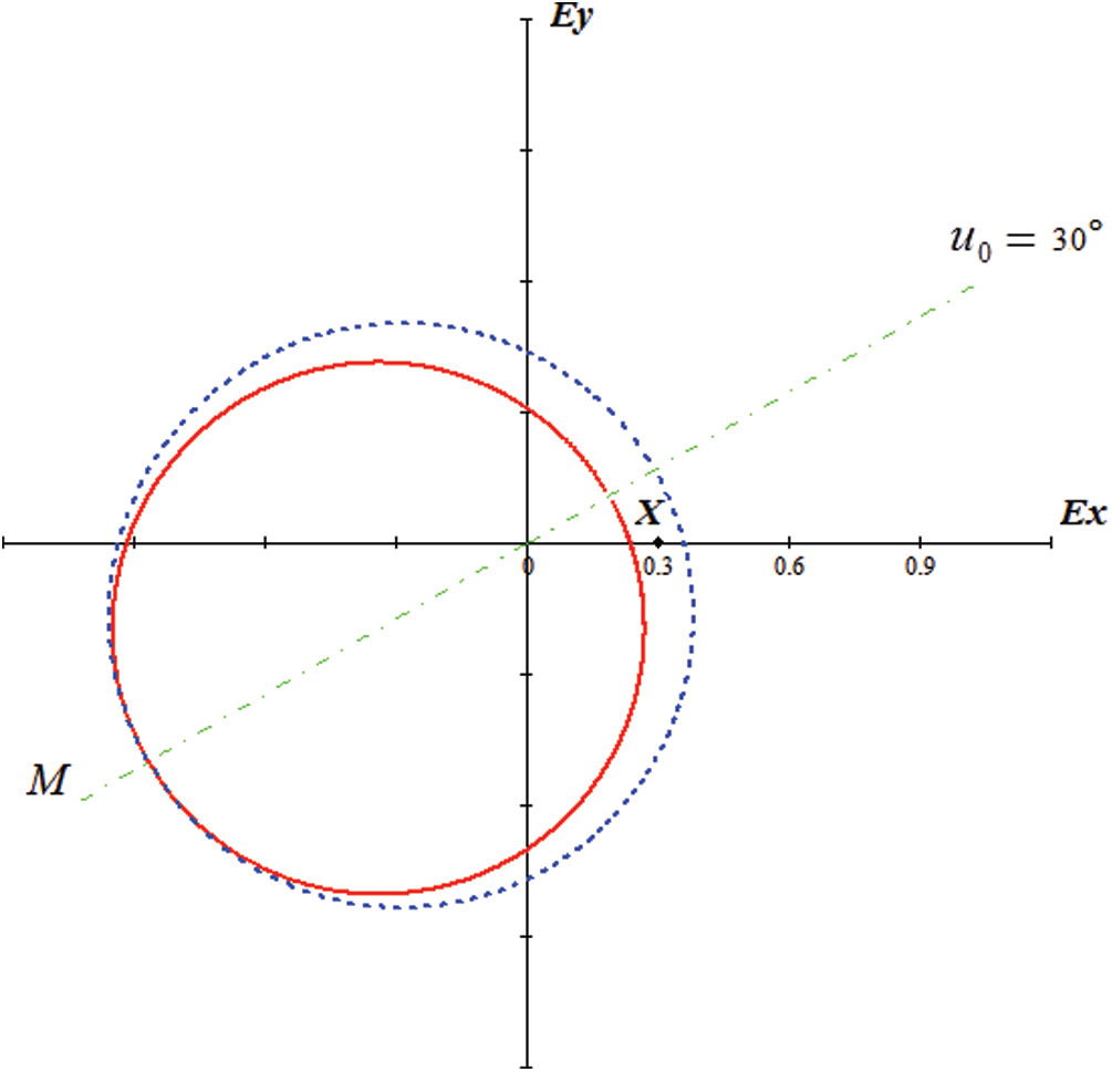
Figure 1: The prohibited area for rendezvous of spacecraft

Fig. 2 shows the prohibited regions if a dangerous approach occurs at angles u0 = 100∘ and u0 = 210∘. The symmetry axis of the prohibited region rotates relative to the origin of coordinate system, meanwhile, position and dimensions of the prohibited region also have changed.

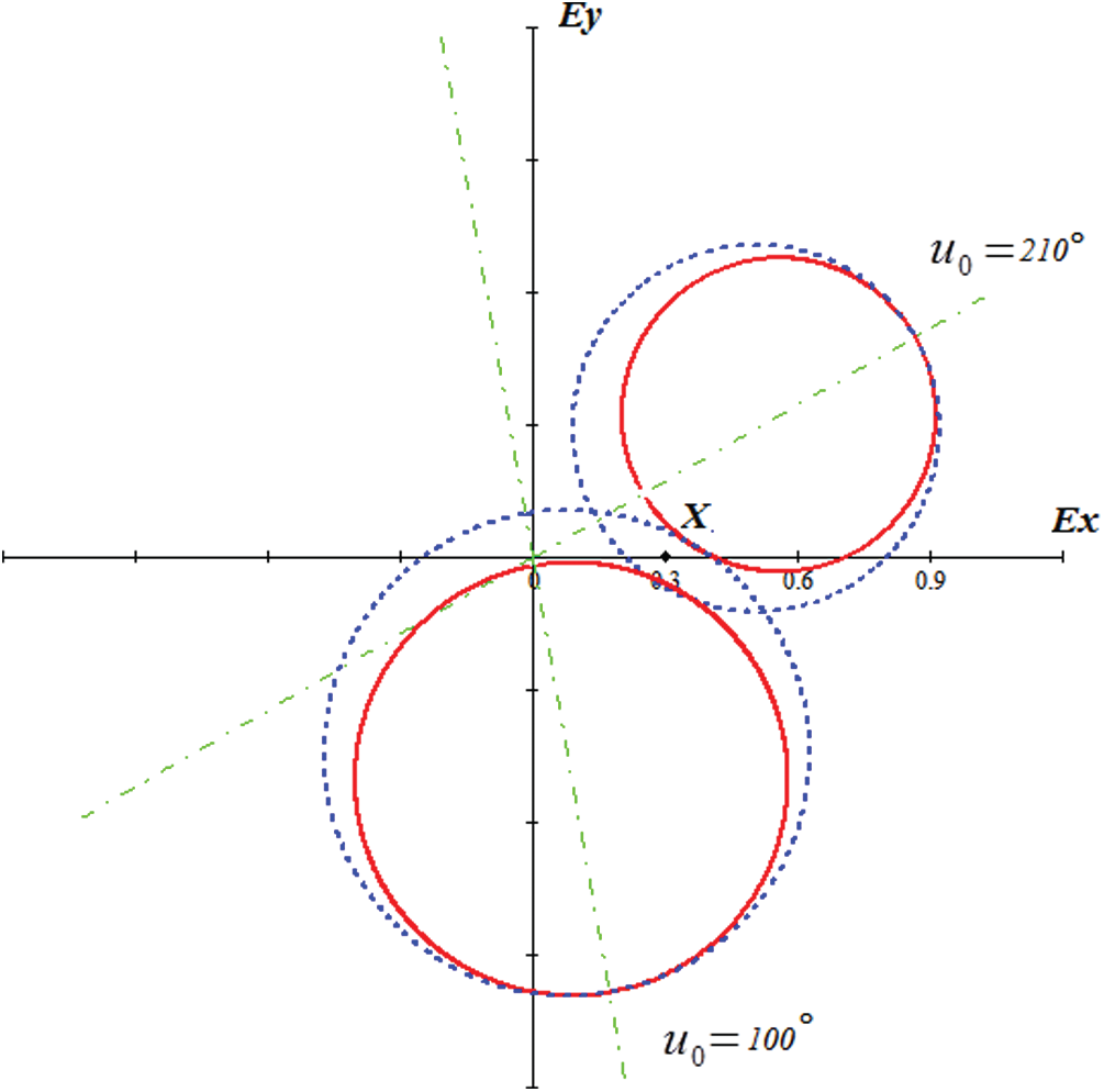
Figure 2: The position of prohibited regions for angles u0=100∘ and u0=210∘

As noted above, the actual value of Δ r is much smaller than that used in these examples presented. In Fig. 3 shows the prohibited region for the phasing orbit of spacecraft “Soyuz” with a0 = 6660 km, eccentricity e0 = 0.005, latitude argument ω0= 135∘, the meeting point with orbital station u0 = 358∘, collision occurs at u0 = 135∘, Δ r = 10 km. It can be seen that in the acceptable range of eccentricity (near the point X (ex0, ey0)), boundary of the prohibited area is approximately linear. Gap of prohibited region is 2Δ e and Δ e can be calculated by the formula as follows:

Δe=Δr/a0(15)

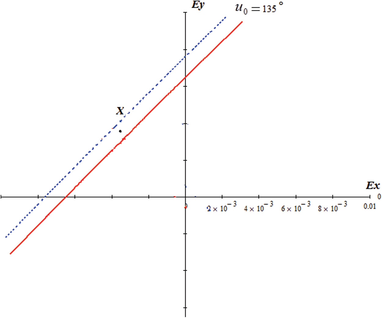
Figure 3: Position of the real prohibited region for angle u0 = 135∘

Based on this scheme, analyses about the position of prohibited region depending on the argument of latitude at which collision occurs can be carried out. In the same coordinate plane, several regions under study that correspond to the possibility of collisions at angles u0 = 0∘, 45∘, 90∘, 135∘. As the position of regions shown in Fig. 4, when the angle u0 changes, prohibited region rotates around point X (ex0, ey0).

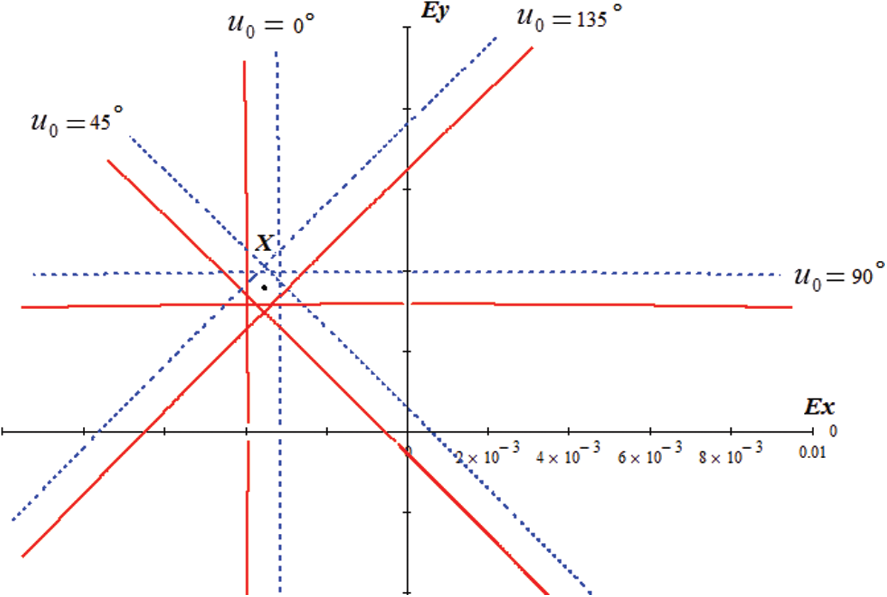
Figure 4: The prohibited region with different angle of u0

Consider an example for the Russian spacecraft “Soyuz” and orbit station “Progress” based on the results obtained previously. In order to ensure a flight to the station vicinity for these spacecraft, a four impulses rendezvous problem is initially solved. All the impulses have transversal components, and lateral components are performed in the first two impulses.

For near circular orbit motion, as described follows from Eqs. (1), (2), a change in the orbit eccentricity vector as a result of the application of transversal component Vti of the i-th velocity impulse on the ex, ey plane can be represented by the vector AB (see Fig. 5). The length of the vector is −2Vti, and forms an angle ϕi with axis ex.

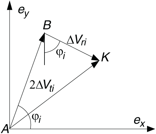
Figure 5: The eccentricity vector change of a velocity impulse

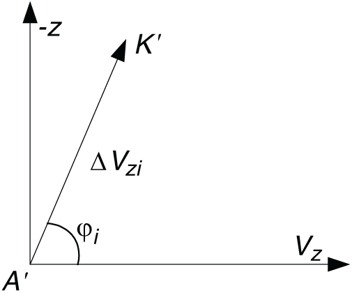
Figure 6: Orbit plane deviation of a normal impulse

From Eqs. (5), (6) it follows that on the plane (Vz, − z) of the normal component of the i-th impulse, which corresponds a vector A′K′ of length Δ Vzi shown with an angle ϕi to the axis Vz (see Fig. 6).

Thus, in multi-impulse solution of the problem in coordinates ex, ey and Vz, − z are expressed as multiple polylines. Similarly, such polylines for a two-impulse solution with zero radial components are shown in Figs. 7 and 8. In this solution, Vt1, Vy2 , Vz1 are positive, Vz2 is negative.

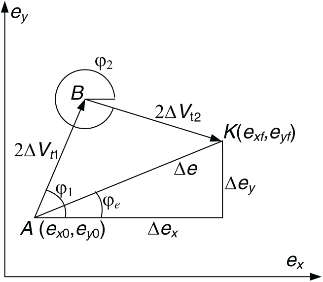
Figure 7: The two-impulses changes of eccentricity vector

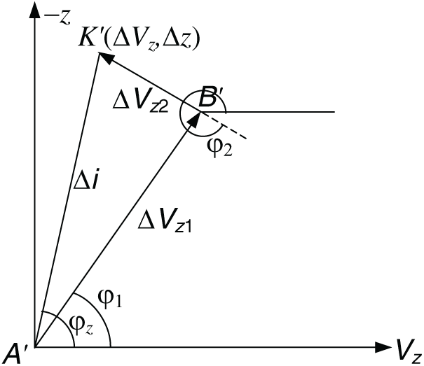
Figure 8: The two-impulses changes for orbit plane

The angle of impulse application is optimal for correcting the deviation of eccentricity vector. The angle of application of the lateral impulse component is optimal for correcting the deviation in the orientation of orbit plane (the impulse is applied on the line of nodes). These angles are calculated by the following formulas:

tgφe=ΔeyΔextgφz=-ΔzΔVz

A four-impulse solution corresponds to a four-link broken line starting in point A and ending in point K. At the optimal initial phase for the transfer flight between non-intersected orbits, the optimal solution should have the same sign for the transversal components of impulse in each of the two maneuvering intervals. Two impulses of the first maneuvering interval correspond to a two-link broken line ABC of length 2VtI, from point A to B. The angles of application of the velocity impulses can be selected arbitrarily, this indicates that point C, corresponding to the eccentricity vector of the waiting orbit formed by maneuvers of the first interval, should belong to a circle of radius R1 = 2|VtI| with a center point A (see Fig. 7). Similarly, for the second maneuvering interval, point B should belong to a circle of radius R2 = 2|VtII| centered at K (see Fig. 8), since a broken CDK with a length of 2VtII corresponds to the second interval maneuvers for a flight from the waiting orbit (AB eccentricity vector) to a given orbit (BK eccentricity vector).

At the optimal initial phase for the optimal transfer flight between non-intersected orbits with radius R1 = 2|VtI| and R2 = 2|VtII|, intersected and have the same sign of VtI, VtII. In this case, there are many solutions with the same dimensionless total characteristic of velocity maneuvers |Δ a|/2. Point C, corresponding to the parameters of the waiting orbits of such decisions, should belong to the set G-the intersection of R1 and R2 circles (see Fig. 9). This is necessary for the signs of transversal velocity components to coincide at each of the maneuvering intervals.

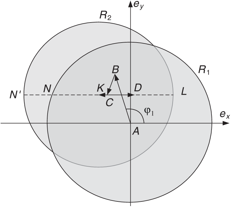
Figure 9: Four impulses solution for rendezvous mission

Solution set with the same V allows to introduce additional restrictions. When calculate the maneuvers of Soyuz spacecraft and Progress, angles of the last two velocity impulses are fixed per revolution and half to the meeting point. Thus, with the impulses of the first maneuvering interval, it is necessary to go to the segment LN which is parallel to the axis ex. The third impulse corresponds to the segment CD, the fourth segment DK. In order to reduce the fuel cost for necessary rotation of orbit plane, angles of velocity impulses in the first maneuvering interval, should be as close as possible to the line of nodes and lie on different sides of it.

With the adopted maneuvering scheme, it is possible to effectively avoid collision if the approaching point is close to the ascending or descending node of the orbit (u0 = 0∘ or u0 = 180∘). In this case, the axis of the prohibited region is parallel to the ordinate axis and passes through point C (Δ ex0, Δ ey0) corresponding to the eccentricity vector of the waiting orbits, obtained after the second impulse (see Fig. 10).

In order to obtain a safe solution, the eccentricity vector of the phasing orbit must be derived from the prohibited region, which is easy to realize by changing the angles of application of the first two impulses; and in order to obtain a solution in which TCV is close to the one of optimal solution, the eccentricity vector of phasing orbit should belong to the intersection region of circles with radius R1 and R2. A solution that satisfies both requirements is shown in Fig. 11.

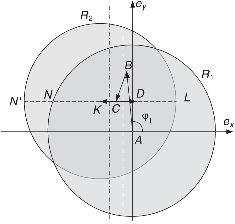
Figure 10: A collision solution with SD in the ascending node of the phasing orbit

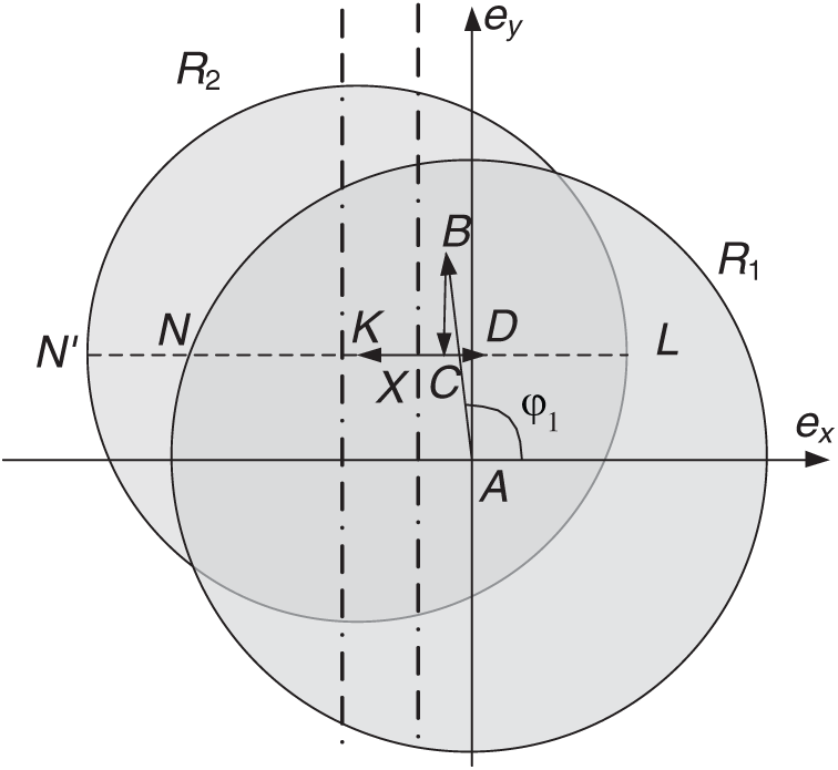
Figure 11: A solution to avoid collision without changing the scheme of maneuvering

Consider a more complicated case, when the point of possible collision is as far from the equator as possible (u0 = 90∘ or u0 = 270∘). The danger zone axis is parallel to the abscissa axis (see Fig. 12).

Without changing the maneuvering scheme (changing the angle of application of the third or fourth pulses), it is impossible to avoid a collision, because the end of the eccentricity vector of the phasing orbit (Δ ex0, Δ ey0) should belong to a straight line passing through the middle of the prohibited area.

As shown in Fig. 13, a collision can be avoided by changing the angle at which one pulse in the second maneuvering interval is applied, and the effect would be better if the application angles of the two impulses in the second maneuvering interval are changed simultaneously. In this way, the eccentricity vector of the phasing orbit will be removed from the danger region.

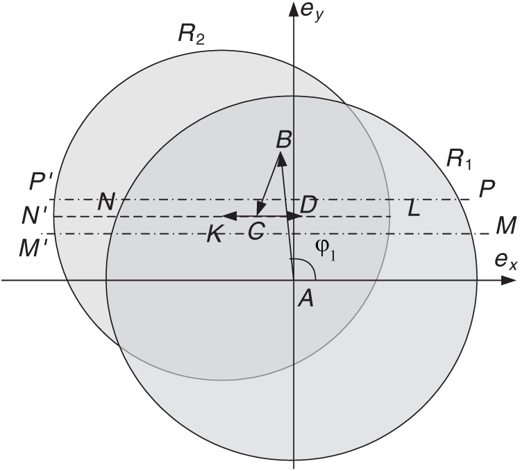
Figure 12: A solution in which a collision with a CM occurs in a phasing orbit

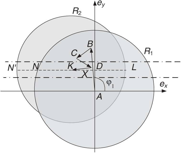
Figure 13: A solution to avoid collision after changing the maneuvering pattern

The area corresponding to collisions at different latitude arguments can also be considered as an option, when in a phasing orbit a collision with several SD objects at different points of the orbit. In slow collisions, the possibility of a collision does not exist at a point, but in a significant range of latitude arguments. The prohibited zone will be restricted to the boundaries line between the two extreme points.

In the slow rendezvous situation, the possibility of collision does not exist at a point, but over a wide range of latitude arguments. The prohibited lane will be limited by straight lines which are the areas boundaries for the two extreme points of the range of possible collisions. An approximate view of the danger area for such a case when a dangerous approach is possible in the latitude range from 60∘ to 120∘ is shown in Fig. 14. The area is enclosed between straight lines N′S and P′S′ on the left side in the figure, and between straight lines SL and S′M on the right side in the figure.

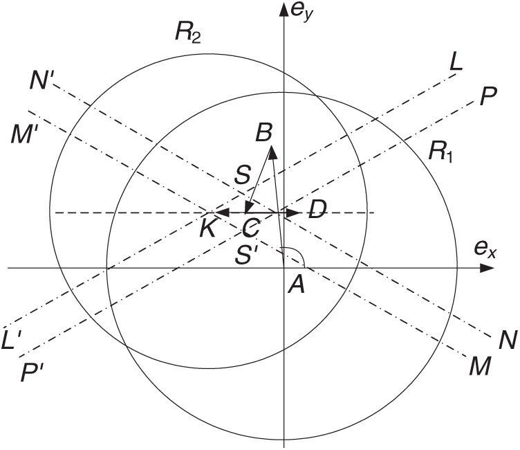
Figure 14: Prohibited area when collision is possible in the range of 60∘ to 120∘

It should be noted that if the eccentricity vector is derived from this area, then the risk of collision in the area from 240∘ to 300∘ is simultaneously eliminated.

The solution to the multi-impulse rendezvous problem for a given class of orbits is usually sought using the simplex method. We can offer two other methods for solving this problem, which have shown their effectiveness [24–27]. The first algorithm [25,26] is also numerical, but rather simple.

The angles of application of the first two impulses of velocity ϕi are sorted out (for spacecraft “Soyuz” and “Progress” correspondingly these impulses are indicated as ϕ1 and ϕ2), When enumerating the allowed maneuvering intervals, the step can be selected 80, such a step allows to find a close result to optimal solution with a small number of options being considered. Then, for each set of angles, the system of four linear Eqs. (1) −(4) is solved, from which the values of the four transverse components of the impulsive velocity can be determined (the radial components of the impulsive velocity are not used); the two values of lateral components of the impulsive velocity are found by system (5)–(6). For each solution, the eccentricity vector of phasing orbit is calculated. For the problem described in this paper, only solutions for which there is no collision remain in consideration, i.e., the eccentricity vector of the phasing orbit does not belong to the prohibited area. The optimal solution among feasible solutions is the one for which the Δ V is minimal. As all numerical methods, in this case there is no explanation for the solution obtained or its absence, it is not clear how to change the maneuvering scheme if necessary.

It is most efficient to obtain the desired solution using a graphical dialogue with a problem. In this scheme, based on the analysis of the above presented, angles of application of any of the velocity impulses can be changed, and thus a compromise solution that displays the eccentricity vector of phasing orbit from the danger area can be obtained. Thus, a compromise solution can be obtained that removes the eccentricity vector of the phasing orbit from the dangerous region, but leaves it in the region of optimal solutions. A solution can be found in which point C will be sufficiently far from the danger area without a significant increase in Δ V.

4  Conclusions

In this paper a fundamentally new approach to calculate maneuvers for avoiding a collision with space debris is proposed, an effective algorithm is proposed for solution changes to the rendezvous problem, which avoids the collision in phasing orbit of the initial optimal solution. It is demonstrated that the protected area from object must be derived is built on the plane of eccentricity vector components. The prohibited region is bounded by two parallel lines, the axis of this region passes through the end of the eccentricity vector of the phasing orbit of the optimal solution. The orientation of the axis depends on the latitude argument at which the collision may occur. The sizes of this region are determined, depending on Δ r as the necessary deviation along the radius of the vector.

The prohibited region and the region of optimal solutions are depicted on the same plane, which allows using a graphical dialogue when solving the rendezvous problem to find a compromise between the desire to avoid the dangerous object as far as possible and to reduce the delta costs that grow with distance from the optimal solution. The proposed approach to solving the problem also makes it quite simple to calculate rendezvous maneuvers, which also provide evasion from several collisions or from “slow” collisions in a phasing orbit, when the protected spacecraft and the SD object fly dangerously close to each other for a long time. The use of the constructed area will allow solving the problem of collision avoidance of a satellite group (Satellite Formation Flying) with a group of space objects.

Data Availability: Both the methodology and simulation data used to support the findings of this study are available from the corresponding author upon request.

Funding Statement: This work is supported and funded by NSFC (Natural Science Foundation of China) [No. 51905272]. The authors would like to thank the editors and the anonymous reviewers for their valuable comments and constructive suggestions.

Conflicts of Interest: The authors declare that there is no conflict of interest regarding the publication of this paper.

This work is licensed under a Creative Commons Attribution 4.0 International License, which permits unrestricted use, distribution, and reproduction in any medium, provided the original work is properly cited.