Computer Modeling in Engineering & Sciences

DOI: 10.32604/cmes.2021.016018

ARTICLE

Comparison of Coarse Graining DEM Models Based on Exact Scaling Laws

Bin Zhang1,2, Yiming Huang3,4 and Tingting Zhao5,*

1School of Economics and Business Administration, Chongqing University, Chongqing, 400030, China
2CMCU Engineering Co., Ltd., Chongqing, 400041, China
3Sichuan University, Chengdu, 610065, China
4China Construction Eighth Engineering Division Corp., LTD Southwest, Chengdu, 610000, China
5College of Mechanical and Vehical Engineering, Taiyuan Univeristy of Technology, Taiyuan, 030024, China
*Corresponding Author: Tingting Zhao. Email: zhaotingting@tyut.edu.cn
Received: 31 January 2021; Accepted: 09 March 2021

1  Introduction

Since the origination of discrete element method (DEM) in 1970s [1], it has been applied to various particulate systems and therefore appeared to be an established approach. The DEM has been demonstrated to be a powerful tool for investigating problems occur in scientific and industrial particulate processes [2–5]. The capability to investigate the phenomena occuring between every single particle is the most attractive feature of DEM while the number of particles is the key factor that influence the calculation speed. The simulation of a large number of particles requires unacceptable computational time that is the most critical problem exists in the industrial application of DEM. The real industrial applications require billions of particles (macro-scale problem) compared with the calculating capability of several million particles (micro-scale problem) on a single personal computer.

The coarse graining technique is a possible approach to tackle the macro scale problem. To put it simply, when using coarse graining in DEM the particles are artificially enlarged in the model which significantly reduces the number of particles in the system therefore the calculation time is acceptable. It is obviously that when use large-sized particles in DEM simulation the performance such as the energy dissipation of the coarse-graining system is not same with the original system. Therefore, when the DEM simulation is performed by using such large-sized particles, some theoretical issues need to be addressed to explain the difference between the original system and the coarse graining system. Moreover, a systemic framework needs to be proposed to develop a reliable coarse graining system which can represent the original system well.

The original system and the coarse graining system are simplified as a rectangular in the Fig. 1. It should be noted that the regular arrangement of the particles here is just for brevity. As we can see, the characteristic dimension of the system keeps the same while the characteristic dimension of the discrete elements has been enlarged. In the previous work [6,7], a parameter as scale number Sn, has been introduced to represent the difference between the original system and the coarse graining system. It is obvious that the scale number of the original system is larger than that of the coarse graining system. While how does this scale number effect the performance of the whole system and how to guarantee the two systems show the similar performance need more discussion.

This problem can be treated from two aspects. On one hand, from the particle level, the governing equation for particle motion and the interaction law involved should be scaled properly. On the other hand, from the system level, the difference caused by the configuration of the particles should be considered. In the exact scaling system, the characteristic dimension of the system and the elements are scaled simultaneously (see Fig. 1). The exact scaling model is a geometrically exact representation of the original problem, i.e., both models have the same particle number and particle packing configuration while this condition cannot be kept between the coarse grainging system and the original system. The coarse grainging system could be seen as a part of the exact scaling system. The particle sizes and the domains in the original and exact scaling models are different only by a constant (spatial) scale factor h. In what follows, the overbar− will be used to denote a quantity associated with the exact scaling system.

Let R and R̄ be the radii of an arbitrary particle in both the original and exact scaled models respectively, and D and D̄ denote the characteristic lengths of the domains in both models. Then R̄=hR; D̄=hD; Sn̄=Sn. In this situation, the scale number Sn remains the same for both models. A set of scaling laws has been proposed to assure that the exact scaled system can exactly represent the original system. The scaling conditions for the exact scaled system is briefly introduced in Section 2. The existing coarse graining techniques developed by other researchers are all intended to keep the similarity between the original system and the scaled system on the particle level. Section 3 aims to compare some of existing coarse grain technologies and evaluate them within our generic theoretical framework based on the exact scaled system.

Then the next step is to tackle this problem on the system level. The equivalent dynamical properties of the original system and the exact scaled system can be guaranteed completely by applying the scaling conditions on the exact scaled system. However, there will be inevitable difference between the coarse grained system and the original system caused by the different packing configurations. It could also be explained that the coarse grained system is only a part of the exact scaled system (see Fig. 1) which will show some differences compared to the whole system. However, such difference has been discussed scarcely in the former research. This paper tries to fill this gap by conducting a series of simulations to figure out the precision of the coarse graining in Section 4 as it is hardly to analyse such difference theoretically.

2  Scaling Conditions for Exact Scaling System

A complete set of scaling conditions under which the exact scaled system can exactly reproduce the behaviour of the original system has been established in the previous work [6,7]. The conditions are derived from the governing equations in a straightforward manner, based on simple unit conversions of all the physical quantities involved in both physical and scaled models.

The mechanical motion of the particle system is fully governed by Newton’s second law. The governing equations for an arbitrary particle can be generally expressed as

mu¨(t)+Fd(t)+Fint(t)=Fext(t)(1)

where m is the mass of the particle, Fd is the damping force accounting for any energy dissipation in the system, Fint is the resultant of all the interaction forces from other particles or other phases defined by the interaction laws, Fext is the resultant external force applied if any, and u¨ is the acceleration.

The governing equations for the particle in the exact scaled system could be written as

m̄u¨̄(t)+F̄d(t)+F̄int(t)=F̄ext(t)(2)

To ensure the results obtained in the exact scaled system can be exactly scaled back to the results for the original system, the above two equations should be mathematically equivalent, or simply differ only by a constant factor. Unlike the classic dimensional analysis or some earlier work on the development of scaling laws for particle systems [8,9], Feng’s previous work takes a relatively simple approach which ensures that all the corresponding forces involved in both systems are proportional:

m̄u¨̄mu¨=F̄dFd=F̄intFint=F̄extFext=λ(3)

A set of scaling laws are established on this basis by a more straightforward approach which aims to determine the scale factors for all the individual physical quantities involved in the particulate system. Let q be an arbitrary physical quantity in the system, and λq is the scale factor for q

q̄=λqq(4)

Physical quantities are interdependent and can be derived from a few basic quantities. The three basic quantities in our work are Length [L], Mass density [ρ] and Time [T] and the corresponding scale factors for these three quantities are specifically chosen as

λL=h;λT=h;λρ=1,(5)

i.e., the scale factors for length and time are the same as the spatial scale factor.

After the scale factors for the basic quantities between the original and exact scaled systems are defined, the scale factors for other quantities can be derived easily as shown in Tab. 1 (see [6] for details). These choices of the scale factor for the basic quantities lead to a desirable result. The scale factors for particle stress, strain, kinetic energy density, strain energy density are unity, which ensures the similarity between the original system and the exact scaled system.

Table 1: Scale factors for some physical quantities in the exact scaling system

Applying these scaling laws into the DEM simulation could be accomplished by two possible ways. One desirable way is to apply the required scale factor to all the quantities involved. Another way named partial scaling approach has been explained elaborately in [7]. Some existing coarse graining approaches of other researchers could be treated as tackling the problem by the latter way.

As the same time-stepping integration scheme will be adopted for the original system and the exact scaled system, it is not difficult to deduce that the scale factor for the time step associated with the scheme should be λΔt=λT=h, which implies that the same number of time steps are required in the exact scaled model as in the original model. In other words, the same computational costs will be involved in solving both original and exact scaled models, and thus the exact scaling offers no computational cost savings.

3  Comparison of Existing Coarse Graining Models

To reduce computational costs for a large scale problem, some non-exact scaling approaches, named as coarse graining methods, have been proposed which can be classified into three categories. The first method develops a specific model in which a large-sized particle is used to represent a group of original particles and then a series of relationships between the original system and the coarse grained system are derived. The particle-fluid system is the main study object of this method. The second method applies dimensional analysis to guarantee the equivalent properties of the two systems based on the motion equation. The third method focus on the interaction law directly.

Although the exact scaling approach cannot improve the calculation efficiency, the scaling laws proposed can serve as the basic principles to guarantee the similar behaviour of particles with different sizes, which is also the objective of other coarse graining approaches. Therefore, it is reasonable to incorporate those coarse graining approaches into the theoretical framework based on the exact scaling system considering its simplicity and general applicability. This feature can be seen more clearly when compared with those existing coarse graining approaches.

3.1 Representative Model

Coarse graining is based on an intuitive thought that a group of small particles could be represented by a large particle to reduce the problem size. The coarse grained model in Fig. 1 is obtained by replacing four small particles by a large particle. The approach based on this concept has been the most commonly used method for coarse graining. The most important feature of this approach is that the particle-particle and fluid-particle interaction forces of the representative particles are calculated using the physical properties of the original particles. Only the detection of contacts or collisions between particles is performed using the diameter of the representative particles. Such forces need to be scaled properly to ensure the similarity between the original system and the coarse grained system. The governing equation of this approach is similar to Eq. (1). Unlike the systemic way that scale factors are obtained in the dimensional analysis, the scale factors here are derived based on a number of assumptions. Here, two models in this category which are cited frequently are investigated in detail.

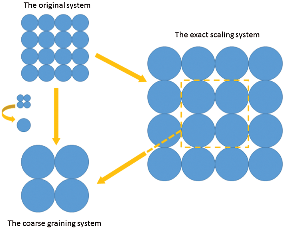
Figure 1: The original system, the exact scaling system and the coarse graining system

3.1.1 Similar Particle Assembly (SPA)

The first one is the similar particle assembly (SPA) model developed by Kuwagi et al. [11] as shown in Fig. 2. The original system consists of a bed of particles. These particles are grouped together in which their size, density, and chemical composition are similar. Their velocity and direction of motion are also similar. The representative system contains a set of representative particles that are assumed to occupy an equal space size with the size h times larger than the original particles. A similar particle assembly model is established because the spatial arrangement of the original system and that of the representative system is analogous. Use i and i′ to denote particle indices in the original system and in the representative system respectively below.

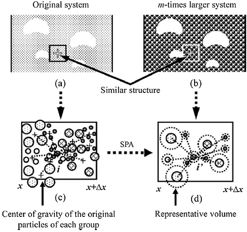
Figure 2: Diagram of the scaling law for the similar particle assembly (SPA) model [10]

The governing equation for particle motion in the original system takes the following form:

ρp(i)(π6dp(i)3)dv(i)dt=∑i≠jFp(ij)+Ffp(i)+ρp(i)(π6dp(i)3)g+Fcoh(6)

where ρp(i) is the particle density, dp(i) is the particle diameter, i,j are the particle indices, Fp(ij) is the contact force between two contacting particles i and j, Ffp(i) is the fluid-particle interaction force, Fcoh is the liquid bridge force. It is easy to figure out that this equation is just another equivalent expression of Eq. (1).

The particle sizes in the representative system and the original system follow the scaling relationship

dp(i′)=hdp(i)(7)

The corresponding equation of (6) for the coarse grained (representative) system becomes

h3ρp(i′)(π6dp(i)3)dv(i′)dt=∑i′≠j′F̄p(i′j′)+F̄fp(i′)+h3ρp(i′)(π6dp(i)3)g+F̄coh(8)

The scaling law for the terms in this equation is proposed subjectively without theoretical analysis. It is believed that the particle diameter has a major impact on the hydrodynamic behaviour of the particle, so the scaling law can be applied directly to particle-particle and particle-fluid interaction forces, as shown below:

∑i′≠j′F̄p(i′j′)+F̄fp(i′)+F̄coh=h3(∑i≠jFp(ij)+Ffp(i)+Fcoh)(9)

The author claimed that if Eq. (9) is satisfied and the density of the space represented by a representative particle is the same as the original particle, then the velocity congruity can be established by further comparing Eqs. (6) and (8) as

v(i′)=v(i)(10)

The advantage of this model is obvious that in the coarse graining system the physical properties of the original particles can be used directly. The diameter of the representative particle is only used when perform the detection of contacts or collisions between particles. To put it simply, the author just applies a scale factor of h3 to all the terms in the governing equation, but there is a contradiction in this SPA model.

From Eq. (10), the author draws the conclusion that particles in the coarse grained system has a motion that is similar to the that of the corresponding original particles. If based on the exact scaling system, the scale factor of length for the SPA model is h, as the scale factor of velocity is 1, thus the scale factor of time is also h, and the same for the scale factor of time step. If we compare the left hand sides of Eqs. (6) and (8), no scaling is applied to the term of dt which is a contradiction between the SPA model and the conclusion based on the exact scaling laws. If a scale factor h is applied to dt, then the total scale factor of the left hand side of Eq. (9) is h2, therefore the force scale factor for the SPA should be changed from h3 to h2.

3.1.2 Coarse Grain Model

To simulate a pneumatic conveying, Sakai et al. [12,13] developed the coarse grain model based on the SPA approach with more details. As described in Fig. 3, there are h3 original particles in the (3D) coarse grain particle whose size is h times larger than the original particle. As shown in Fig. 3a the translational motion of the coarse grain particle is assumed to be the same as that of the group of original particles. Therefore, the velocity and displacement of the coarse grain particle is assumed to be the average of those of the original particles. As far as the rotational motion is concerned, the original particles existing in the coarse grain particle each are assumed to rotate around their own center of mass with the same angular velocity, as illustrated in Fig. 3b. The contact force acting on the coarse grain particle is estimated under the assumption that the kinetic energy of the coarse grain particle agrees with that of the original particles. The drag force and external force are modeled by balancing the coarse grain particle with the group of the original particles. For the cohesive particles, the van der Waals force is modelled based on the assumption that the potential energy of the coarse grain particle is the same as the original particles. Consequently, the following relationship is obtained between the coarse grain particles and the original particles.

mCGMv̇CGM=FfCGM-VCGM∇p+∑ FCCGM+FgCGM+FvwCGM=h3FfO-h3VO∇p+h3∑ FCO+h3FgO+h2FvwO(11)

where m,v,h,Ff,V,p,FC,Fg and Fvw indicate mass, velocity, scale factor, drag force, particle volume, pressure, contact force, gravitational force and van der Waals force respectively. The subscripts of CGM and O refer to coarse grain particles and original particles, respectively.

Figure 3: Coarse grain model (a) Translation (b) Rotation [12]

According to the author, the scale factor h3 for the contact force is obtained under the assumption that when a binary collision in coarse grain particles occurs, the binary collisions due to all the original particles (i.e., h3 binary collisions) are assumed to occur simultaneously. While based on the exact scaling laws, to ensure that the scale factors for particle stress, strain, kinetic energy density, strain energy density are unity, the scale factor for force should be h2 rather than h3. The contact forces caused by the binary collisions cannot be added up directly because contact forces of the interior particles counteracts with each other and are cancelled out. The resultant force for a group of original particles is only the sum of the forces provided by the particles on the exterior boundary with other groups of particles. It means that the force of the coarse grain particle is more like an area integral rather than a volume integral.

The scale factor of the van der Waals force is h2 which satisfies the exact scaling laws. It is derived by the assumption that the potential energy of the coarse grain particle is the same as that of the original particles. The relationship of the potential energy between the two systems is given by

∫FipCGM(lCGM)dlCGM=h3∫F̄ipO(lO)dlO(12)

where l indicates the inter-surface distance.

The relation between the inter-surface distance of the coarse-grain particles and the original particles is expressed as

lO=lCGMh(13)

From the above two equations, a long-range force acting on the coarse grain particle can be generally expressed as

FipCGM(lCGM)=h2F̄ipO(lO)=h2F̄ipO(lCGMh)(14)

Consequently, the long-range van der Waals force acting on the coarse-grain particles is given as

FvdwCGM=h2F̄vdwO(15)

The scale factors for different types of force are different in this coarse grain model because different assumptions are used to derive the scale factors. The assumption which leads to the scale factor h2 is from the point of energy equivalence between the two systems, a fundamental physical quantity that should be kept similar. With this consideration, the scaling laws for the drag force and other external forces are also inappropriate.

Another problem in this particular coarse grain model is the time step Δt. We can find the following relation in [12]

Δt<2πmCGM/kCGM=2πh3mO/h3kO=2πmO/kO(16)

This relation is not correct since all the original physical properties are used in the coarse grain model which means that kCGM is equal to kO not h3kO. Then the relationship of the time step in the two systems can be written as

ΔtCGM=h3/2ΔtO(17)

From this relation, we know that the coarse graining method improves the computational efficiency by both reducing the number of particles and enlarging the time step.

In conclusion, when all the physical properties of the original particles are used in the coarse grain model, every force term in the equation of motion should be scaled by h2.

3.2 Dimensionless Analysis

This approach could be regarded as the extension of the classic dimensional analysis [8,9] to the DEM simulation. Firstly, the governing equation of the particulate system is written in dimensionless form. A set of non-dimensional quantities are sought from which a set of scaling laws can be identified. The detail of the dimensionless analysis can be found in the paper of Pöschel [14] which presents the method to scale down experiments to lab-size. The procedure is shown below along with the comparison with the exact scaling approach. Consider the equation of motion below:

d2δdt2+BmR(δ3/2+32Aδdδdt)=0δ|t=0=0dδdt|t=0=v0(18)

which is an equivalent form of Eq. (1) for a contact pair. The interaction force is given by Hertz’s law shown in the second term on the left side where B is the elastic constant

B=2E3(1-ν2)(19)

The damping force (refer to [15]) is shown in the third term where A is the dissipative material constant as a function of the viscous constants η1,2, the Young modulus E and the Poisson ratio ν.

A=13(3η2-η1)23η2+2η1(1-ν)(1-2ν)Eν2(20)

To write down the above equation of motion in a dimensionless form, a characteristic length and a characteristic time are needed. The maximal compression δ0 is chosen as the characteristic length. It can be found by equating the kinetic energy of the impact with the elastic energy at the instant of the maximal compression

mv022=mBmR25δ05/2(21)

which yields

δ0=(54mRB)2/5v04/5(22)

The characteristic time is defined as the time in which the particles move the distance of the characteristic length just before the collision starts

t0=δ0v0(23)

the rescaled length, time, velocity, and acceleration are expressed as

δ^=δδ0(24)

t^=tt0=tv0δ0(25)

dδ^dt^=dδ^dδdδdtdtdt^=1v0dδdt(26)

d2δ^dt^2=d(1v0dδdt)dtdtdt^=δ0v02d2δdt2(27)

So, the equation of motion can be written in the dimensionless form below:

d2δ^dt^2+54δ^3/2+32(54)3/5A(BmR)2/5v01/5δ^dδ^dt^=0δ^|t^=0=0dδ^dt^|t^=0=1(28)

To make the two systems behave identically, the value of the elastic constant B and dissipative constant A should be conserved by scaling the material properties involved. After conducting a complicated dimension analysis, the author derives that the scale factor of elastic constant is h and that of the dissipative constant is h when the scale factors of length and time are h and h, respectively.

The above procedure can be incorporated into the exact scaling system. The three basic quantities are also length, time and density. If we set δ0=h then t0=h, it is easy to derive the scale factors of the elastic constant and the dissipative constant based on the exact scaling system. The dimension of the elastic constant B is [ρ][L]2[T]-2, therefore the scale factor should be h. Similarly, the dimension of the dissipative constant A is [ρ][L]2[T]-1/[ρ][L]2[T]-2, thus the scale factor should be h.

In the work of Bierwisch et al. [16], such dimensional analysis has been adopted and three dimensionless numbers are obtained as

Π1=wRE,Π2=γnRρE,Π3=κtRE(29)

where w is the surface energy density, γn is the empirical damping parameter and κt is the tangential spring constant. Thus, the scaling laws for the material properties involved are

w∝R,γn∝R,κt∝R(30)

There is a slight difference on the choice of the basic quantities when using our scaling system to explain the above approach. The three basic quantities in their work are length, density and Young’s modulus with the three scale factors h, 1 and 1. The scale factor for Young’s modulus is decided to ensure that the energy density dissipation rates are unaffected by coarse graining.

The three basic quantities chosen here are an equivalent form to the choice of the exact scaling system. That is why the scaling factor for the material properties here are the same with the corresponding term listed in Tab. 1. It is necessary to point out that the scaling laws in that exact scaling system keeps the energy density conserved between the original system and the scaled system.

This dimensionless analysis was also applied to the simulation of gas-particle flows for dense particle regions by Radl et al. [17]. This work is continued by Nasato et al. [18] who extended the analysis for the Hertz model and a limited analysis in the cohesive contact model.

3.3 Modification of Interaction Laws

Some researchers focused on the scaling of model parameters in contact interaction laws to produce scale independent predictions in numerical simulations. Thakur et al. [19] investigated the scaling law for cohesionless and cohesive solids under quasi-static simulation of confined compression and unconfined compression to failure. The work of Yun et al. [20] suggests the scaling rule for static liquid bridge model to reasonably simulate the fluid-like behaviour of particles.

This type of approach is even more a one-sided methodology which cannot take the entire features of the whole system into consideration. Different scaling laws for just one quantity may be obtained by this method. We can find this situation in [19] for cohesive systems, where different equations for inter-particle forces are proposed, leading to a contradiction conclusion that the cohesive force should be scaled linearly, squarely or cubically with the radius of the particle respectively based on different interaction laws.

Consider the adhesive force f0 that can be calculated based on three different equations.

1) From the equation,

f0=AR6s2(31)

where A is the Hamaker’s constant, s is the separation distance between the particles.

The author only realised that the radius of the particle R is a scale related quantity while ignored the scale factor for the distance s. It is suggested that the adhesive force should be linearly proportional to the radius of the particle.

Considering the dimension of distance s, the force should be scaled squarely proportional to the radius of the particle.

2) From the equation

f0=4πR2ϕkσt(32)

where ϕ is the packing fraction, k is the coordination number and σt is the tensile strength.

Based on this equation, it is suggested that the force should be scaled with the square of the particle radius, which is correct as all the quantities apart from R in the equation are dimensionless.

3) From the equation

f0=fg=43πR3ρg(33)

This suggests that the force should be scaled cubically with the radius of the particle. The dimension of gravity g is neglected because the author regards the radius R as the only factor which has an influence on the cohesive force with upscaling.

The simulation results based on the three methods above show that the quadratic scaling produces very similar behaviour between the original system and the scaled system which demonstrates again that the force should be scaled by a factor h2.

4  The Precision of the Coarse Graining System

From the discussion above we know that the scale factor should be h2 when λL=h and λρ=1. There will be unavoidable difference between the original system and the coarse grainging system as disscussed above. It is meaningful to understand how the scale factor will affects the simulation results. A series of simulations has been conducted to figure out the statistical regularity of this difference of which the theoretical analysis is difficult. The biaxial test is preferred to estimate the precision of the quasi-static process of the coarse graining system.

The simulations of biaxial tests are conducted using the PFC2D software. The scale factor of length λL for a series of scaled systems begins from 2 and increases by a step of 10% except for the last one 4. The distribution of particle size follows the Gaussian distribution. The packing information for each scale are listed in the Tab. 2. As it can be seen that the number of particles in the coarse grainging system decreases squarely with λL which will improve the computational speed significantly. The height, width and porosity of all the packings are same as 12, 6 and 0.2. All the other physical quantities involved in the simulation are scaled by the scaling laws according to their dimensions in exact scaling system.

Table 2: Packing information for each scale

Since the configuration of all the packings is random, 20 samples for each scale have been created in our analysis. Fig. 4 illustrates the variation of average contact force with axial strain for each scale. The value for each sample is shown in the solid line with different colours.

Figure 4: Variations of average contact force with axial strain for all the samples of each scale

The dimension and scale factor for the average contact force Fave could be derived as

[Fave]=[ρ][L]4[T]-2;λFave=h2(34)

While in the two-dimension situation, the above equation is changed to

[Fave]2D=[ρ][L]3[T]-2;λFave2D=h(35)

This relation gives rise to the theoretical value for the average contact force which is shown as red circles in Fig. 4 for each scale. For each scale, the variation of average contact force with axial strains shows the same trend. All the values fluctuate around the theoretical value while the ranges of fluctuation extend as the scale factors increase. It gives us a qualitative conclusion that the precision of the coarse graining system reduces as the scale factor increases.

To analyse the precision quantitatively, the gradient of average contact force to axial strain is preferred as the index for comparison. The theoretical values and the values calculated by the numerical simulations for all the scales are listed in Tab. 3. The computational results are the average of the results of 5 samples, 10 samples and 20 samples, respectively.

Table 3: Packing information for each scale

The relative error between the theoretical value and the computational result is obtained by

err=|Gtheory-Gaverage|Gtheory(36)

Fig. 5 shows the relationship between the average of the relative error of the gradient and the scale factor. The diagrams illustrate this relationship based on the results from 5 samples, 10 samples and 20 samples, respectively. As we can see, the trend of this relation obtained from the computational results of 5 samples is not obvious. The error shows a more obvious growing tendency as the scale factor increase in the right digram (20 samples) from 2% of λL=2 to 3% of λL=4.

Figure 5: The relationship between the relative error of the gradient and the scale factor

Figure 6: The relationship between the variance relative error of the gradient and the scale factor

While in the right diagram of Fig. 5, there still some points deviate from the growing tendency. The variance of hte error could explain this phenomenon in some ways. The realtionship between the variance of the relative error and the scale factor is shown in Fig. 6. It shows the same result that as the number of the samples increases the relation between the variance and the scale factor is more obvious. In the right diagram, the variance of λL=2.2 is almost 0.016 which gives the variation range of the error of λL=2.2. As in the right diagram of Fig. 5, the error of λL=2.2 is 0.03, the possible range for this error is 0.03±0.016. This range is too large so that the value for this scale deviates from the growing tendency. To achieve a tendency more stable, more samples for each scale need to be created to reduce the randomness of the packing configuration.

5  Conclusion

In this paper, some existing coarse graining methods have been analysed by the exact scaling law. The basic principle to guarantee the original system equivalent to the scaled system is to make the equation of motion for each system proportional to each other. The technique used in the representative model is to keep all the quantities with the same values in both the original system and the scaled system. Then the equation of motion for the scaled system is scaled by a factor proposed artificially based on different assumptions. Unreasonable assumptions easily lead to an inappropriate scale factor. The dimensionless analysis reaches this goal by extending the equation of motion based on the specific interaction laws used in different applications and proposing different dimensionless parameters accordingly. This procedure is complicated sometimes and may not be applied directly to other applications. The method of modifying the interaction law has not considered the scaling problem form this basic principle. The scale factor of the force is proposed only based on the relationship between the force and the particle size of hte specific interaction law.

While in the exact scaling system, the equivalent of the original system and the scaled system can be achieved by simply scaling each quantity involved by a scale factor which can be easily derived according to its dimension. By applying these laws, a series simulations of biaxial compression tests with different scale factors have been conducted to investigate the precision of the coarse graining system. The error of the original system and the coarse system shows a growing tendency as the scale factor increases. It can be concluded that the precision of the coarse grainging system is accepted when apply scaling rules based on the exact scaling laws.

Acknowledgement: The authors wish to express their appreciation to the reviewers for their helpful suggestions which greatly improved the presentation of this paper.

Funding Statement: This work is partially supported by National Natural Science Foundation of China under Grant No. 12072217. The support is gratefully acknowledged.

Conflicts of Interest: The authors declare that they have no conflicts of interest to report regarding the present study.

This work is licensed under a Creative Commons Attribution 4.0 International License, which permits unrestricted use, distribution, and reproduction in any medium, provided the original work is properly cited.