Computer Modeling in Engineering & Sciences

DOI: 10.32604/cmes.2021.014460

ARTICLE

Solution and Analysis of the Fuzzy Volterra Integral Equations via Homotopy Analysis Method

Ali. F. Jameel*,1, N. R. Anakira2, A. K. Alomari3 and Noraziah H. Man1

1School of Quantitative Sciences, Universiti Utara Malaysia, Kedah, Sintok, 06010, Malaysia
2Department of Mathematics, Faculty of Science and Technology, Irbid National University, Irbid, 2600, Jordan
3Department of Mathematics, Faculty of Science, Yarmouk University, Irbid, 21163, Jordan
*Corresponding Author: Ali. F. Jameel. Email: alifareed@uum.edu.my
Received: 29 September 2020; Accepted: 25 February 2021

1  Introduction

Integral equations have been used to model problems in a number of fields [1–4]. In real-world problems, inaccuracy, uncertainty and lack of information exist and are discussed both theoretically and numerically. The way to address this lack of information is to model uncertainty as fuzziness [5]. It is therefore possible to refer to fuzzy integral equations rather than to use deterministic models in the crisp domain. In order to study and solve many of the problems in applied mathematics, integral equations in fuzzy form are important, particularly for physics, for medical modelling [6]. In many applications, certain problem parameters are typically defined by a fuzzy number rather than a crisp number, and it is therefore important to establish mathematical models and numerical procedures for the proper handling of fuzzy integral equations. Numerical approaches to fuzzy integral equations have inspired many research works in the last decade due to their use in scientific phenomena [7–11]. The existence and uniqueness of a second kind fuzzy Volterra equation solution was introduced in [12]. Among the approximate methods for fuzzy Volterra integral equations, there are the Differential Transform Method (DTM) to obtain analytical solution of linear fuzzy Volterra integral equations of second kind [13], Homotopy Perturbation Method (HPM) for solving linear and nonlinear fuzzy Volterra integral equations of second kind [14,15] and Variational Iteration Method (VIM) together with Taylor method to solve linear fuzzy Volterra integral equations of second kind [16]. The main application of fuzzy integral equations is biomathematical modelling. For example, a model based on fuzzy integral equations [16] was proposed to study the dynamics of diseases transmitted through direct contact between susceptible and infected individuals. Solving mathematical problems with approximation methods usually lead to approaches in series or polynomial functions which often have a better interpretability and this can contribute to pave the way to future processes and solutions of given problems, without the shortcoming of a suitable discretization. In the 90s, Liao introduced a new approximation approach called homotopy analysis method [17]. The approximate solution is obtained as an infinite series function that has been shown to converge to the exact solution in many mathematical problems involving engineering applications [18–22]. The homotopy, a fundamental concept in topology, is a landmark of the approximation methods, since it provides more flexibility in handling the equations and their solution [23]. The validity of HAM depends on homotopy topology, regardless of the physical parameters. It is worth recalling that the Adomian Decomposition Method (ADM) and the VIM are non-perturbation techniques, which do not depend on a series of physical parameters, but such non-perturbation techniques in some cases do not guarantee the convergence of the solution series [24]. The HAM also allows to select the proper base function without any constraint to approximate the solution of some nonlinear problems [25].

The difference between HAM and other approximation methods is the auxiliary convergence control parameter, denoted by h, that can optimize and rate the convergence of the method per order of solution [26]. In HAM the selections of proper initial approximation, operator and auxiliary function with the optimal value of h allows to solve the deformation equations and develop a solution series [20].

To control the error of HAM solution, there is a convergence-control parameter, whose value, if properly selected, can lead to an accurate convergent series or faster convergence [27]. Van Gorder et al. [28] discussed the application of HAM for nonlinear ordinary differential equation and the effectiveness of a suitable choice of initial approximation, auxiliary linear operator, auxiliary function and convergence control parameter. There are several methods to obtain the best value of the convergence-control parameter such as control of residual errors, minimization of error functional and optimal selection of the homotopy of auxiliary function which were introduced and suggested for the approximate solution of semi-linear elliptic equation in [29]. Moreover, an algorithm was proposed in [30] to optimize the solution of singular and integral equation of first kind via HAM by computing the optimal auxiliary control parameter value.

HAM has been used to solve several types of problems in crisp and fuzzy domains, e.g., fluid flow and heat transfer problems [31], fractional differential equations involving biological models [32], system of nonlinear ordinary differential equations describing HIV infection models [33], Abel’s integral equations of the first kind [34], fuzzy boundary value problem [35] and fuzzy delay differential equation [36].

The present work deals with the approximate solution of fuzzy Volterra integral equations of second kind, since to the best knowledge of the authors no study has been carried out by formulating the general concept of HAM from the crisp domain to the fuzzy domain for solving such class problems.

The paper is structured as follows. The Volterra integral equations of the second kind with the defuzzification details are recalled in the next section. A new description of the fuzzy HAM general formula is presented in Section 3, where a convergence analysis is also outlined. In Section 4, some test problems are considered and the numerical results discussed. Finally, there is a short conclusion that includes a summary of this work. Note that some of the basic fuzzy definitions, remarks and concepts not described in this paper are well-known. Notions of fuzzy level sets, fuzzy numbers and their operations, fuzzy functions, fuzzy Zadeh extension theory and integral of fuzzy functions can be easily retrieved from the literature, e.g., [9,37–41].

2  Fuzzy Volterra Integral Equation

The general fuzzy version of the standard second kind Volterra integral equation [9] is defined below:

x̃(t)=f̃(t)+λ̃∫atk̃(t,s,x̃(s))ds,(1)

where λ̃ is a positive fuzzy parameter, k̃ is an arbitrary function called the kernel of the integral Eq. (1) defined over square G:[a,b]×[a,b], k̃=0, a≤s, t≤b, s > t and f̃(t) is a given fuzzy function of t∈[a,b] with x̃(s) is the unknown fuzzy function to be determined.

Eq. (1) follows the properties of the standard second kind Volterra integral equation in crisp domain by means of defuzzification according to [9]. Hence, Eq. (1) with the fuzzy parametric forms are given as follows:

x̃(t;r)=f̃(t;r)+λ̃(r)∫atk̃(t,s,x̃(s;r);r)ds,(2)

where

{x̃(t)=x̃(t;r)=[x(t;r),x¯(t;r)],f̃(t)=f̃(t;r)=[f(t;r),f¯(t;r)],λ̃=λ̃(r)=[λ(r),λ¯(r)],k̃(t,s,x̃(s))=k̃(t,s,x̃(s);r)=[k(t,s,x(s;r);r),k¯(t,s,x¯(s;r);r)],x̃(s)=x̃(s;r)=[x(s;r),x¯(s;r)].(3)

with 0≤r≤1. By using Eq. (3), the solution of Eq. (1) can be obtained by solving the following two integral equations:

{x(t;r)=f(t;r)+λ(r)∫axk(t,s,x(s;r);r)dsx¯(t;r)=f¯(t;r)+λ¯(r)∫axk¯(t,s,x¯(s;r);r)ds(4)

The sufficient conditions for the existence of a unique solution to Eq. (2) are given and proved in [11].

3  General Fuzzy HAM

The crisp form of HAM was introduced in [42]. To describe the dynamic of the HAM under homotopy theory in the fuzzy domain, we start off with:

N[x̃(t;r)]=0,(5)

where N is a nonlinear operator, t is an independent variable and, x̃(t;r) is an unknown fuzzy function. According to [14], the zero-order fuzzy deformation HO for all r∈[0,1]:

HO(t;p;r)=(1-p)L[θ̃(t;p;r)-x̃0(t;r)]-ph̃(r)H(t)N[θ̃(t;p;r)],(6)

where p∈[0,1] is an embedding parameter, h̃(r)≠0 is a convergence-control parameters per each r level sets. Function H(t)≠0 is an auxiliary function, L is an auxiliary linear operator, x̃0(t;r) is the fuzzy initial guess of x̃(t;r) and θ̃(t;p;r) is the auxiliary function that should satisfy the initial conditions. It should be noted that the h̃(r) and H(t) are necessary to the HAM series solution rate of the convergence [17]. The parameter p changes from 0 to 1 to generate series solution such that when p = 0, one has

HO(t;0;r)=L[θ̃(t;0;r)-x̃0(t;r)]=0,(7)

while if p = 1, one gets

HO(t;1;r)=ph̃(r)H(t)N[θ̃(t;1;r)]=0.(8)

Thus, by imposing

HO(t;p;r)=0,(9)

It is

(1-p)L[θ̃(t;p;r)-x̃0(t;r)]=ph̃(r)H(t)N[θ̃(t;p;r)].(10)

From [13], if p = 0 and p = 1, the homotopy equations becomes

{θ̃(t;0;r)=x̃0(t;r),θ̃(t;1;r)=x̃(t;r).,(11)

As p changes from 0 to 1, the fuzzy solution θ̃(t;p;r) varies from the initial guess x̃0(t;r) to the HAM solution x̃(t;r). By expanding θ̃(t;0;r) as a Taylor series in terms of p, we can yield the series solution in the following form:

θ̃(t;p;r)=x̃0(t;r)+∑m=1∞x̃m(t;r)pm,(12)

where

x̃m(t;r)=1m!∂mθ̃(t;p;r)∂pm|p=0.(13)

The auxiliary linear operator L, the initial guess x̃0(t;r), the convergence control h̃(r) and the auxiliary function H(t) are very important for the best homotopy series solution. Note that if p = 1 then we have

θ̃(t;1;r)=x̃0(t;r)+∑m=1∞x̃m(t;r)pm,(14)

which is one of the solutions of the given equation to be solved by HAM. Notice that if all the values of h̃(r)=-1 and H(t)=1 then Eq. (10) takes the form:

(1-p)L[θ̃(t;1;r)-x̃0(t;r)]+pN[θ̃(t;1;r)]=0,(15)

which represents the homotopy perturbation method (HPM), implying that HPM is a special case of HAM [43]. From Eq. (10) the governing equations can be deduced from the zero-order deformation Eq. (12) by defining the vectors:

x̃i→(t;r)={x̃0(t;r),x̃1(t;r),…,x̃m(t;r)}.(16)

By deriving with respect to p both sides of Eq. (10) m times, at = 0, and after that dividing them by m!, we obtain the mth-order deformation equation

L[x̃m(t;r)-χmx̃m-1(t;r)]=h̃(r)Rm(x̃m-1→(t;r)),(17)

where

Rm(x̃m-1→(t;r))=1(m-1)!∂m-1N[θ̃(t;p;r)]∂pm-1|p=0,χm={0,m≤11,m>0.(18)

4  Fuzzy HAM for Fuzzy Volterra Integral Equations

In this section, the HAM solution of fuzzy Volterra integral equations is described in some steps.

Construct the zeroth-order deformation for Eq. (1) for all r∈[0,1] as:

(1-p)L[x̃(t;p;r)-f̃(t;r)]=ph̃(r)[x̃(t;p;r)-f̃(t;r)-λ̃(r)∫atk̃(t,s,x̃(s;p;r);r)ds].(19)

Set the values of p = 0 and p = 1, implying

{x̃(t;0;r)=f̃(t;r),x̃(t;1;r)=x̃(t;r).(20)

From Eq. (20), it follows that the fuzzy initial guess x̃0(t;r) can be selected from f̃(t;r) as there are no restrictions to select the proper HAM initial guess to obtain the suitable solution of any given equation [17]. According to Section 3, the Taylor series in terms of p for x̃(t;p;r) is:

X̃(t;p;r)=x̃(t;0;r)+∑m=1∞x̃m(t;r;h̃(r))m!pm,(21)

where x̃m(t;r;h̃(r))=1m!∂mx̃m(t;r;p;h̃(r))∂pm|p=0. Now for p = 1 in Eq. (21) the mth-order deformation equation is obtained:

X̃(t;r)=f̃(t;r)+∑m=1∞x̃m(t;r;h̃(r))m!.(22)

From the mth-order deformation equation

x̃m(t;r)=χm-1x̃m-1(t;r)+h̃(r)[x̃m-1(t;r)-∫0t(λ̃(r)k̃(t,s,x̃m-1(s;r);r))ds-(1-χm-1)f̃(t;r)],(23)

χm={0,m≤11,m>0, one obtains

x̃1(t;r;h̃(r))=h̃(r)x̃0(t;r)-h̃(r)f̃(t;r)-[h̃(r)∫0t(λ̃(r)k̃(t,s;x̃0(s;r);r))ds],(24)

where x̃0(t;r) is the initial guess obtained from f̃(t;r) and for m≥2, we have:

x̃m(t;r;h̃(r))=(1+h̃(r))x̃m-1(t;r;h̃(r))-[h̃(r)∫0t(λ̃(r)k̃(t,s,x̃m-1(t;r;h̃(r));r))ds].(25)

Then the fuzzy HAM series solution can be written in the following form:

X̃(t;r;h̃(r))=x̃0(t;r)+∑m=1∞x̃m(t;r;h̃(r))={x0(t;r)+∑m=1∞xm(t;r;h(r)),x¯0(t;r)+∑m=1∞x¯m(t;r;h¯(r)).(26)

The convergence of Eq. (26) depends on selecting a suitable value of h̃(r). The solution is therefore obtained in series form (homotopy solution series):

X̃(t;r)= limm→∞∑m=0∞x̃m(t;r).(27)

It is worth noticing that since the defuzzification leads to a system of crisp equations, the theoretical achievements on the convergence in [30] can be adapted.

5  Dynamics of Fuzzy HAM Convergence

As mentioned before, the convergence of the approximate solution of Eq. (1) relies on the value of the parameter h̃(r). Therefore, the value of h̃(r) should be sought to provide sufficient accuracy for a certain order of the HAM series solution. The procedure is to define first Eq. (26) in residual form:

R̃(t;r;h̃(r))=X̃(t;r;h̃(r))-f̃(t)-λ̃∫atk̃(t,s,X̃(t;r;h̃(r)))ds.(28)

then to use the least square method to optimize the values of h̃(r) such that:

S̃(t;r;h̃(r))=∫at(R̃(t;r;h̃(r)))2dt.(29)

After that, the nonlinear equation coming from Eq. (29) in terms of h̃(r) for any r∈[0,1] is deduced such that:

∂S̃(t;r;h̃(r))∂h̃(r)=0→{∂S(t;r;h(r))∂h(r)=0∂S¯(t;r;h¯(r))∂h¯(r)=0.(30)

Finally, the equation is solved for h̃(r) in each fuzzy level set to obtain the best value of h̃ to be replaced in Eq. (26), in order to rate the convergence of the HAM solution. Hence, one needs to estimate the best value of h̃(r) to get the best approximate solution X̃(t;r;h̃(r)). This can be done by plotting the h-curves for all r∈[0,1]. These curves can help to find the region ℂ which contains the best values of h̃(r)∈ℂ. If there exist c0∈[0,T], by plotting the quantities R̃(t;r;h̃(r)), X̃m(x,h̃(r);r), X̃m′(c0;r;h̃(r)), X̃m″(c0;r;h̃(r)) and so on for -2<h̃(r)<0, it is possible to find the valid region ℂ. The latter is known to be delimited by the line nearly parallel to the horizontal axis [17]. According to [35,36] the best value of h̃ can be selected from the fuzzy level set r = r0 with highest accuracy and then replaced in the remainder for the optimal upper and lower bound solutions of Eq. (1).

The HAM for seeking the approximate solution of Eq. (1) can be summarized in the following algorithm.

Step 1: Set the initial guess x̃0(t;r)=x̃0(x̃0=[x0,x¯0]).

Step 2: Set the value of λ̃(r)=[λ(r),λ¯(r)].

Step 3: Set number of terms, s.t. i=1,2,…,j.

Step 4: Set i = i + 1 and for i = 1 to i≤j evaluate

x̃i(t;r)=χi-1x̃i-1(t;r)+h̃(r)[x̃i-1(t;r)-∫0t(λ̃(r)k̃(t,s,x̃i-1(s;r);r))ds-(1-χi-1)f̃(t;r)].

Step 5: Compute

X̃(t;r;h̃(r))=∑k=0jx̃i-1(t;r).(*)

Step 6: Set the fixed value of r0∈[0,1] and t∈[a,b]; evaluate

h̃(r0)=∂X̃(t;r0;h̃(r0))∂h̃(r0), then plot the h-curve (-2≤h≤0).

Step 7: Define the residual form in Eq. (28) and use Eqs. (29)–(30) to find the best value of h̃(r0); then substitute the values of h̃(r0) in Eq. ( * ) to detect the optimal value of h̃(r0).

Step 8: Replace again the optimal value of h̃(r) for the lower and upper level in Eq. ( * ).

6  Application Examples

In this section application examples are presented. For the remainder of this work, Er̃ and MEr̃ will denoted the absolute error and the mean error respectively, defined as follows:

Er̃(t,r;h̃)=|XX̃(t;r)-X̃(t;r;h̃)|={|XX(t;r)-X(t;r;h̃)||XX¯(t;r)-X¯(t;r;h̃)|(31)

MEr̃(t,r;h̃)=Er(t,r;h̃)+Er¯(t,r;h̃)2(32)

Example 6.1: Consider the following linear fuzzy Volterra integral equation [13]:

x̃(t)=f̃(t)+∫0x(t-s)x̃(s)ds,(33)

where f̃(t;r)=(1-t-t22)[r,2-r] and its exact solution

XX̃(t;r)=[r,2-r](1-sinh(t)).(34)

The HAM formulation (see Section 5) for Eq. (33) is:

x̃m(t;r)=χm-1x̃m-1(t;r)+h̃(r)[x̃m-1(t;r)-∫0t((t-s)x̃m-1(s;r))ds-(1-χm-1)(1-t-t22)[r,2-r]],(35)

where the initial guess x̃0(t;r)=f̃(t;r). By following the analysis in Section 4 and according to [36], for fixed values of the r-level set, namely r = 0.6, the h̃(r)-curves of fifth-order fuzzy HAM upper and lower bound solutions X̃(t,h̃(r);r) for Eq. (33) are shown in the following figures.

Figure 1: Fifth-order fuzzy HAM solution h̃(r)-curves of Eq. (33) at r = 0.6

From Fig. 2, the range of the valid values of h̃ (graph line almost parallel to the horizontal axis) for the fifth-order fuzzy HAM solution is -1.5≤h̃(0.6)≤-0.6. From Eq. (30) the best valid values of h̃ are listed in Tab. 1.

Fig. 3 shows the absolute errors defined in Eq. (31) of the fifth-order fuzzy HAM solution for the values h̃(r) in Tab. 1.

Figure 2: Fifth-order fuzzy HAM solutions accuracy for different values of h̃(0.6)

To be more precise regarding the convergence of HAM, if the values of h̃(0.6) are selected such that h̃(0.6)∉[-1,5,-0.6], e.g., h̃(0.6)=1 or h̃(0.6)=-3, the plots in Fig. 3 are obtained.

From Fig. 3, one can easily deduce that for values of h̃(r) not in the convergence region, one obtains a divergent HAM solution. From Fig. 2, one can notice that h̃2=-1.0039263129319256 is the optimal value of the convergence control parameters among those in Tab. 1. Therefore, Tabs. 2–5 will display the solutions and accuracy of Eq. (33) via fifth-order HAM as follows.

Table 1: Best values of the convergence control parameter of fifth-order fuzzy HAM solution of Eq. (33) at r = 0.6

Figure 3: Fifth-order fuzzy HAM solutions for two different values of h̃(0.6)

Table 2: Fifth-order HAM lower solution and accuracy of Eq. (33) at t = 1 and h̃=h2 for all r∈[0,1]

Table 3: Fifth-order HAM lower solution and accuracy for Eq. (33) at t = 1 and h̃=h2 for all r∈[0,1]

Table 4: Fifth-order HAM upper solution and accuracy for Eq. (33) at t = 1 and h = 1 for all r∈[0,1]

Table 5: Fifth-order HAM upper solution and accuracy for Eq. (33) at t = 1 and h=h¯2 for all r∈[0,1]

From Figs. 4, 5 one can notice that the fifth-order fuzzy HAM solutions of Eq. (31) are in the form of fuzzy numbers for any r∈[0,1] and any t∈[0,1].

Figure 4: Fifth-order fuzzy HAM solution for h=h̃2 and exact solution of Eq. (33) at t = 1, r∈[0,1]

Figure 5: Fifth-order HAM solution for h=h̃2 and the exact solution of Eq. (33) for t∈[0,1] and r∈[0,1]

Example 6.2: Consider the following linear fuzzy Volterra integral equation [16]:

x̃(t)=[r,2-r]cos(t)+∫axet-sx̃(s)ds,(36)

The exact solution of Eq. (36) is given by

XX̃(t;r)=[r,2-r](35cos(t)+15sin(t)+25e2t).(37)

The HAM formulation of Eq. (36) is:

x̃m(t;r)=χm-1x̃m-1(t;r)+h̃(r)[x̃m-1(t;r)-∫0t(et-sx̃m-1(s;r))ds-(1-χm-1) cos(t)[r,2-r]],(38)

where the initial guess is assumed to be x̃0(t;r)=[r,2-r]. The h̃(r)-curves of sixth-order fuzzy HAM upper and lower bound solutions at r = 0.8 for Eq. (36) are shown in Fig. 6.

Figure 6: h̃(r)-curves of the sixth-order fuzzy HAM solution of Eq. (36) at r = 0.8

The valid values of h̃ from Fig. 6 are clearly in the range -1.5≤h̃(0.8)≤-0.6. From Eq. (30) the best valid values of h̃ are listed in Tab. 6.

Table 6: Best values of the convergence control parameter of sixth-order fuzzy HAM solution of Eq. (36) at r = 0.8

From Fig. 7, one can see that the optimal value of the convergence control parameters in Tab. 6 is h̃2. Tab. 7 and 8 show the sixth-order HAM approximate solution of Eq. (36) for t=[0,π8] and r∈[0,1].

Figure 7: Sixth-order fuzzy HAM solution accuracy for some values of h̃ (0.8), t∈[0,π8]

Table 7: Sixth-order HAM solution of Eq. (36) at t=π8 and h = −1 for r∈[0,1]

Table 8: Sixth-order HAM solution of Eq. (36) at t=π8 and h=h̃2 for r∈[0,1]

In Tab. 9 there is a comparison of the mean errors by HAM, VIM and Taylor expansion method [16] (all of sixth-order) at t=π8 for r∈[0,1].

Table 9: Absolute mean error for the solution of Eq. (36) at =π8, r∈[0,1], by the sixth-order HAM approximate, Taylor expansion method and VIM [16]

Clearly from Tab. 9 one can see that sixth-order HAM solution at the optimal value of the convergence control parameter h̃2 is more accurate than the one by VIM and Taylor expansion method for r∈[0,1]. The results in Tabs. 7–8 can be summarized in Figs. 8–9 as below:

Figure 8: Sixth-order HAM for value h=h̃2 and the exact solution of Eq. (36) at t=π8 for r∈[0,1]

Figure 9: Sixth-order HAM solution for h=h̃2 and the exact solution of Eq. (36) for t∈[0,π8] and r∈[0,1]

Example 6.3: Find the solution of the following nonlinear fuzzy Volterra integral equation:

x̃(t)=f̃(t)+∫0xt2(t-2s)(x̃(s))2ds,(39)

where

f(t;r)=(2-r)2(t66+t5-t3+t22)-t22+rt+r,f¯(t;r)=r2(t66+t5-t3+11t232)+(2-r)(-(2-r)11t232+t+1).

The HAM formulation of Eq. (39) is:

x˜m(t;r)=χm−1x˜m−1(t;r)+h˜(r)[x˜m−1(t;r)−∫0t(t2(t−2s)∑j=0m−1x˜j(s;r)x˜ m−1−j(s;r))ds  −(1−χm−1)], (40)

where the initial guess x̃0(t;r)=[r,2-r]. In this example, we introduce the residual error to show one of the HAM advantages to check the accuracy of Eq. (39):

R̃(t;r;h̃(r))=X̃(t;r;h̃(r))-[f(t;r),f¯(t;r)]-∫att2(t-2s)(X̃(s;r;h̃(r)))2ds.(41)

The h̃(r)-curves of the fifth-order fuzzy HAM upper and lower bound solutions at r = 1 of Eq. (39) are shown in Fig. 10.

Figure 10: h̃(r)-curves of fifth-order fuzzy HAM solution of Eq. (39) at r = 1

From Fig. 10 the valid values of h̃ are in the range -1.5≤h̃(1)≤-0.6. The only value of h̃ obtained from Eq. (39) is h̃1=-1.0127292274597477 for the lower and the upper bound solutions. Therefore, Fig. 11 display the accuracy of Eq. (39) via fifth-order HAM as below:

Figure 11: Fifth-order fuzzy HAM accuracy for some values of h̃(1), t∈[0,0.5]

Tabs. 10–13 shows the fifth-order HAM approximate solution of Eq. (39) and accuracy for different values of r∈[0,1] at t = 0.5 and can be summarized in Figs. 12–13 as below.

Table 10: Fifth-order HAM lower solution and accuracy for Eq. (39) at t = 0.5 and h = −1 for r∈[0,1]

Table 11: Fifth-order HAM lower solution for Eq. (39) and accuracy at t = 0.5 and h=h1 for r∈[0,1]

Table 12: Fifth-order HAM upper solution of Eq. (39) and accuracy at t = 0.5 and h = −1 for r∈[0,1]

Table 13: Fifth-order HAM upper solution for Eq. (39) and accuracy at t = 0.5 and h=h¯2 for r∈[0,1]

Figure 12: Fifth-order HAM solution for h=h̃1 and the exact solution of Eq. (39) at t = 0.5, r∈[0,1]

Figure 13: Fifth-order HAM solution for h=h̃1 and the exact solution of Eq. (39) for t∈[0,0.5] and r∈[0,1]

Example 6.4: Consider the following linear fuzzy Volterra integral equation [9]:

x̃(t)=[r2+r,4-r2-r](cosh(t)-λsinh2(t))+λ∫0x sinh(t)x̃(s)ds,(42)

The exact solution for Eq. (42) is given by

XX̃(t;r)=[r2+r,4-r2-r]cosh(t).(43)

The HAM formulation of Eq. (42) is:

x̃m(t;r)=χm-1x̃m-1(t;r)+h̃(r)[x̃m-1(t;r)-∫0t(sinh(t)x̃m-1(s;r))ds-(1-χm-1)([r2+r,4-r2-r](cosh(t)-λsinh2(t)))],(44)

where the initial guess is assumed to be x̃0(t;r)=[r2+r,4-r2-r]. The h̃(r)-curves of the fifth-order fuzzy HAM upper and lower bound solutions at λ=1 and r = 0.4 of Eq. (42) are shown in Fig. 14.

Figure 14: h̃(r)-curves of the fifth-order fuzzy HAM solution accuracy of Eq. (42) at r = 0.4

The valid values of h̃ from Fig. 14 are in the range -1.4≤h̃(0.4)≤-0.7. From Eq. (42) the best valid values of h̃ are listed in Tab. 14.

Table 14: Best values of the convergence control parameter of the fifth-order fuzzy HAM solution of Eq. (42) at r = 0.4

After testing the values of h̃ in Tab. 14, it turned out that the optimal value is h̃1=[h1,h¯1] (see Fig. 15).

Figure 15: Fifth-order fuzzy HAM solution for some values of h̃(0.4), t∈[0,1]

In Tab. 15, there is a comparison of the absolute errors and the results by fifth-order HAM at h̃1 and numerical solution via Trapezoidal quadrature formula (TQF) [9] with number of approximate iterations N = 300 when λ=1 and t = 0.5 for different values of r∈[0,1].

Table 15: Absolute error by fifth-order HAM approximate solution of Eq. (42) for r∈[0,1] and TQF [9] at t = 0.5

From Tab. 15 one can see that the fifth-order HAM solution at the optimal value of the convergence control parameter h̃1, for r∈[0,1], is more accurate than the one by TQF [9] with number of approximate iterations N = 300 at t = 0.5. The results of fifth-order HAM approximation at h̃1 for the lower and the upper bound solutions when λ=1 for all r∈[0,1] and 0≤t≤1 are depicted in Figs. 16 and 17.

Figure 16: Fifth-order HAM solution for h=h̃1 , r∈[0,1], and exact solution of Eq. (42) at t = 1

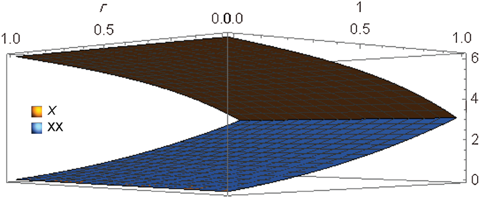
Figure 17: Fifth-order HAM solution for h=h̃1, r∈[0,1]. and the exact solution of Eq. (42) for t∈[0,1]

7  Conclusions

This paper proposes HAM for solving fuzzy Volterra integral equation of the second kind with separable kernels. The fuzzy set theory was used to present a new formulation of HAM with application to the fuzzy Volterra integral equation of the second kind. The convergence of this approach was qualitatively discussed to find the optimal value of the convergence-control parameter. The examples presented show the potential of the method. Numerical results and graphs show that both linear and nonlinear fuzzy Volterra integral equations of the second type are well approximated by the method. Being a semi-analytical method, this approach has the advantage of lead to solutions in explicit form. The numerical experiments showed better performance of the method when compared against other approximation or numerical approaches such as VIM, the Taylor method and the Trapezoidal Quadrature Formula. Due to its accurate results, which do not violate the fuzzy sets theory solution, and a relatively low computational cost, HAM seems to be a reliable tool for solving fuzzy Volterra integral equation of the second kind. In future work, we will apply the approach to some problems in Biomathematics, such as cancer growth and epidemics.

Funding Statement: Dr. Ali Jameel and Noraziah Man are very grateful to the Ministry of Higher Education of Malaysia for providing them with the Fundamental Research Grant Scheme (FRGS) S/O No. 14188 that supported this research.

Conflicts of Interest: The authors declare that they have no conflicts of interest to report regarding the present study.

This work is licensed under a Creative Commons Attribution 4.0 International License, which permits unrestricted use, distribution, and reproduction in any medium, provided the original work is properly cited.