Engineering & Sciences
| Computer Modeling in Engineering & Sciences |
DOI: 10.32604/cmes.2021.014988
ARTICLE
Regarding on the Fractional Mathematical Model of Tumour Invasion and Metastasis
1Department of Mathematics, CHRIST (Deemed to be University), Bengaluru, 560029, India
2Faculty of Engineering and Architecture, Kirsehir Ahi Evran University, Kirsehir, 40500, Turkey
3Department of Mathematics, Faculty of Science, Davangere University, Shivagangothri, Davangere, 577007, India
4Department of Mathematics and Science Education, Faculty of Education, Harran University, Sanliurfa, 63050, Turkey
5School of Information Science and Technology, Yunnan Normal University, Kunming, 650500, China
*Corresponding Author: Wei Gao. Email: gaowei@ynnu.edu.cn
Received: 14 November 2020; Accepted: 09 February 2021
Abstract: In this paper, we analyze the behaviour of solution for the system exemplifying model of tumour invasion and metastasis by the help of q-homotopy analysis transform method (q-HATM) with the fractional operator. The analyzed model consists of a system of three nonlinear differential equations elucidating the activation and the migratory response of the degradation of the matrix, tumour cells and production of degradative enzymes by thetumour cells. The considered method is graceful amalgamations of q-homotopy analysis technique with Laplace transform (LT), and Caputo–Fabrizio (CF) fractional operator is hired in the present study. By using the fixed point theory, existence and uniqueness are demonstrated. To validate and present the effectiveness of the considered algorithm, we analyzed the considered system in terms of fractional order with time and space. The error analysis of the considered scheme is illustrated. The variations with small change time with respect to achieved results are effectively captured in plots. The obtained results confirm that the considered method is very efficient and highly methodical to analyze the behaviors of the system of fractional order differential equations.
Keywords: Tumour cell; invasion and metastasis; q-homotopy analysis transform method; Caputo–Fabrizio derivative
The existence of cancer among the people around the globe has been developed swiftly, and globally it becomes the second foremost cause of demise after cardiovascular diseases [1]. The process of spreading and formation of secondary tumours is known as Metastasis and this nature of cancer cells is the main reason for the death in cancer patients. In addition, the prediction of size, stage, and evolution of a tumour is very critical for the treatment of cancer. Moreover, mathematics plays as an essential tool and aid us to analyze the behaviour of the tumour. The tumour growth has been mathematically modelled by the number of researchers and which are appeared in the literature [2–4]. The growth of the tumour invasion and metastasis are described by PDEs. Particularly, deterministic diffusion-reaction equations and these equations are employed to model the spatial spread of tumours at the initial development and later invasive moments [5].
The fractional-order derivatives are introduced by Leibnitz soon after the classical order derivatives. As compared to classical calculus, it was soon discovered that fractional calculus (FC) is more appropriate for describing real-world problems [6–10]. The calculus of arbitrary order turned out one of the most essential tools to describe biological phenomena. The human diseases which are modelled through derivative having fractional-order help us to incorporate the information about its present and past states [11–16]. Moreover, these models demonstrate the non-local distributed effects, hereditary properties and system memory. These properties are necessary to describe the biological models. In connection with this, recently many authors established the arbitrary-order model to analyze the diffusion equation and to forecast the effect of the tumour and they applied many powerful methods to find the solution for these models [17–32]. The pivotal aim of generalizing the integer to fractional order is to capture consequences related non-locality, long-range memory and time-based properties and also anomalous diffusion aspects. Many real-world problems exemplified with complex and nonlinear models are effectively, systematically and accurately illustrated and investigated by the aid of theory and fundamental concept of FC. Many pioneers nurtured and developed novel and distinct notions of fractional order for both differential and integral operators. Most familiarly hired operators to analyze many models are Riemann, Liouville, Caputo, Fabrizio and others. However, researchers pointed out some limitations while generalizing the system with these notions. The Riemann–Liouville derivative fails to elucidate the essence of initial conditions; the Caputo derivative has overcome this limitation and latter it has been widely applied to the numerous classes of mathematical models exemplifying real-world problems. But this fractional operator is unable to describe the singular kernel of the systems or problems. However, Caputo et al. [33] in 2015 overcome the foregoing obliges and then the number of authors employed CF derivative to investigate and study wide classes of complex and nonlinear problems. It has been proved by many researchers; CF fractional operator as great results compared to other fractional operators.
The study of mathematical models effectively exemplified diverse phenomena. However, as much as important of nurturing the phenomena with the system of equations finding the corresponding solution is also very vital and difficult. In this path, many authors examined diverse phenomena, for instance, the structured predator-prey model with prey refuge [34], COVID-19[35–39], Zika virus transmission [40], planar system-masses in an equilateral triangle [41], a harmonic oscillator with position-dependent mass [42], time fractional Burgers equation [43], fractional optimal control problems [44], Emden–Flower type equations [45], and many others [46–53]. These investigations help researchers to understand the importance of generalizing the classical concept into fractional operators, and efficiency and difference between diverse schemes.
Many physicists, engineers and mathematicians recently proposed and modified diverse solution procedure with a different approach with respect to increasing in accuracy and methodology, to reduces the complexity, many additional assumptions and consideration, huge time for evaluation and to save computer memory. Moreover, each method is suitable for some specific family of problems and they have their own limitations, including conversion of nonlinear to linear, partial to ordinary differential equations, splitting complex and nonlinear term to simple parts terms. In this connection, with the help of topological concept called homotopy, Liao Shijun who is a Chinese Mathematician proposed algorithm called homotopy analysis method (HAM) and illustrated to confirm it overcomes almost all the limitations raised while we solving nonlinear systems exists in sciences and other disciplines associated to mathematics [54]. The most familiar thing of employing this method by many authors is including it solves nonlinear problems without linearization and perturbation.
As science and technology-enhanced, mankind always expecting new tools or modifications in existing tools to improve the accuracy and reduces the time taken for finding needful. In this regard, some scholars pointed out similar things in HAM and suggested to union with existing and familiar transformation. Authors in [55] modified
In the present study, we find the series solution for a system of nonlinear differential equations describing the model of tumour invasion and metastasis using
The rest of the manuscript is organized as follows: The basic and fundamentals are presented in the next section, the hired model is exemplified in Section 3, the basic procedure of the
The basic definitions are presented in this segment for the FC and Laplace transform. Specifically, we recall the notions related to Caputo-Fabrizio fractional operator [33,73].
Definition 1.The CF fractional derivative for
where
Definition 2. The CF fractional derivative for
Note: According to [73], the following must hold
which gives
Definition 3. The
On the basis of generic solid tumour growth and assuming it is in avascular stage, the mathematical model has been proposed [74]. In this stage, most of the tumours are asymptomatic and further there is a possibility of cells to migrate and escape to the lymph nodes. The considered system exemplifies the interfaces of the surrounding tissue with the tumour and it can be extended to incorporate tumour and the vasculature. Here, the projected system of equations illustrates the interactions of the matrix-degrading enzymes (MDE, signifies by
where
where
For the tumour cell density
and for the cell proliferation absence, the equation describing tumour cell motion is defined as
For the notation, the random motility coefficient of tumour cell is considered as
Active MDEs are formed by
where
From the above description, the system is presented as [18,54,57]:
Here, with appropriate initial conditions, Eq. (10) is assumed to satisfy on a region of tissue or domain
where
where
The projected model can be protracted to integrate interactions between blood vessels and the tumour cells [74].
Now, we modify the time derivative by the CF derivative in Eq. (12) and given by
where
4 Fundamental Idea of the Considered Scheme
In this section, we hired the differential equation to present the basic procedure of the projected scheme with initial conditions
and
We obtained by applying LT on Eq. (15)
For
where
where
By using Taylor theorem we get
where
For the proper chaise of
After differentiating Eq. (19)
where the vectors are defined as
Eq. (24) reduces after employing inverse
where
and
Here,
By the help of Eqs. (26) and (27), we found
By the help of
5 Implementation of the
Consider the system of equation cited in Eq. (13) describing the tumour invasion and metastasis in CF fractional derivative
Applying Laplace transform on Eq. (32) and then with the help of Eq. (13), we get
The non-linear operator
The
where
On employing inverse LT on Eq. (35), it simplifies to
By using
6 Existence and Uniqueness of Solutions
In this section, the existence and uniqueness are illustrated for the considered system with the assist of fixed-point theory. We consider the Eq. (32) as follows:
Now, using Eq. (32) and results derived in [53], we obtained
Then we have from [73] as follows:
Theorem 1. The kernel
Proof. Let us consider the two functions
where
Eq. (43) provides the Lipschitz condition for
By the assist of the above equations, Eq. (41) simplifies to
Then we get the recursive form as follows:
The associated initial conditions are
Now, between the terms, the successive difference is defined as
Notice that
Then we have
Application of the triangular inequality, Eq. (50) reduces to
The Lipschitz condition satisfied by the kernel
Similarly, we have
By the help of above result, we state the following theorem:
Theorem 2. If we have specific
Proof. Let
Therefore, for the obtained solutions, continuity and existence are verified. Now, to prove the Eq. (54) is a solution for Eq. (32), we consider
Let us consider
This process gives
Similarly, at
As
Next, for the solution of the projected model, we prove the uniqueness. Suppose
Now, employing the norm on the above equation we get
On simplification
From the above condition, it is clear that
Hence, Eq. (61) proves our required result.
7 Error Analysis of the
Theorem 3. Let
Proof: Let
For every
But
Theorem 4. The maximum absolute error for the series solution of the Eq. (15) defined in Eq. (31) is determined as
Proof: By using Eq. (62), we get
But
This ends the proof.
Table 1: Description of parameters presented in the projected system [74]
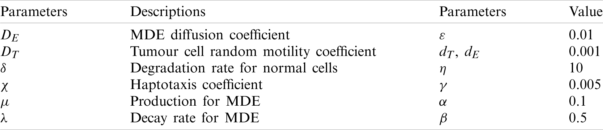
Here, we demonstrate the future scheme is efficient and reliable and evaluate the approximate results for the system of partial differential equations representing a model of tumour invasion and metastasis. In the present study, we find the fourth-order solution to present the nature of the system. In Tab. 1, we present the specific values of the parameters cited in Fig. 1 captures the behaviour of
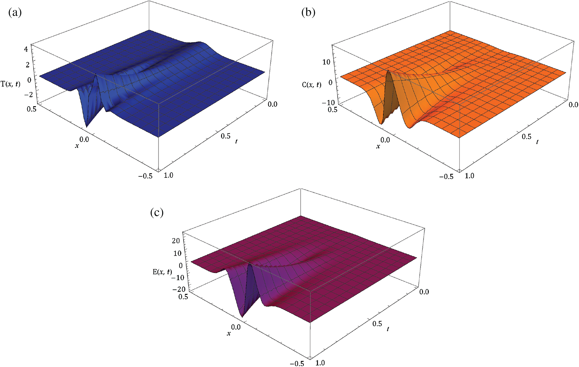
Figure 1: Surfaces of
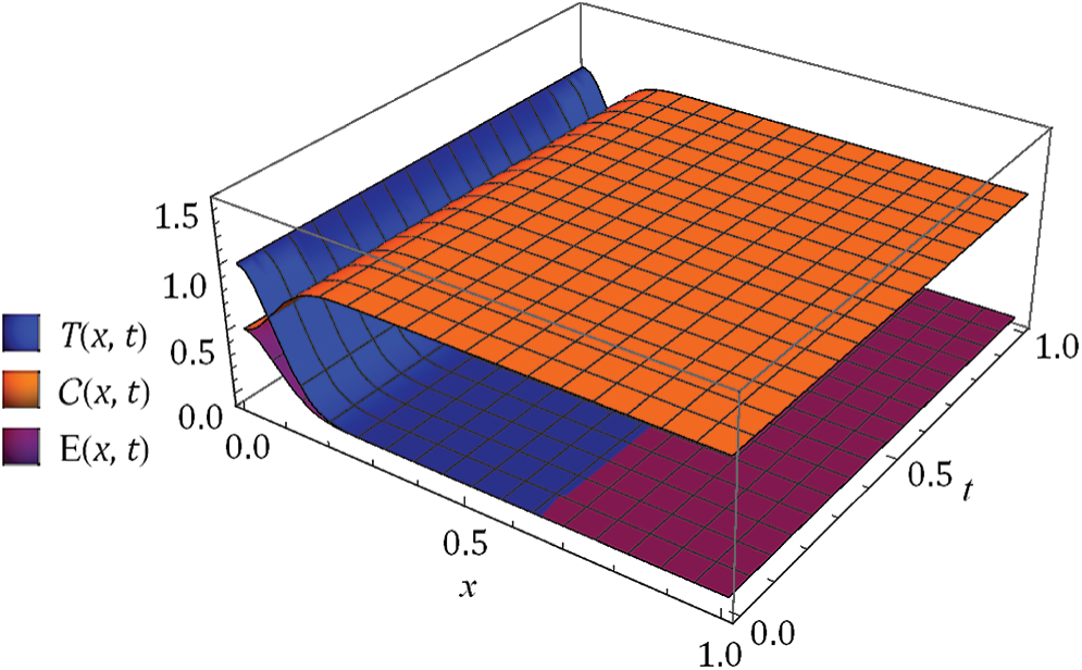
Figure 2: Surface of
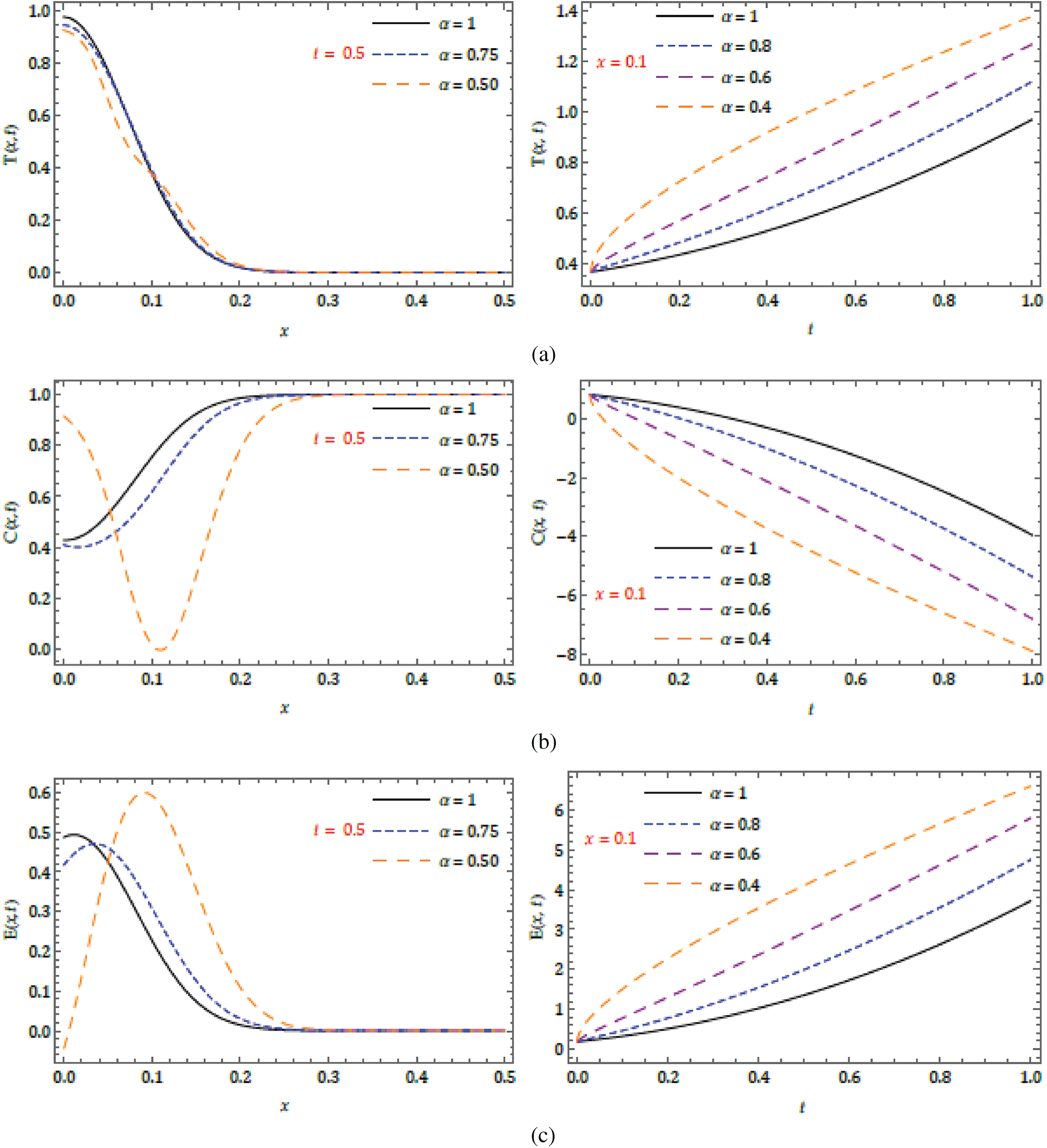
Figure 3: Nature of obtained solution for
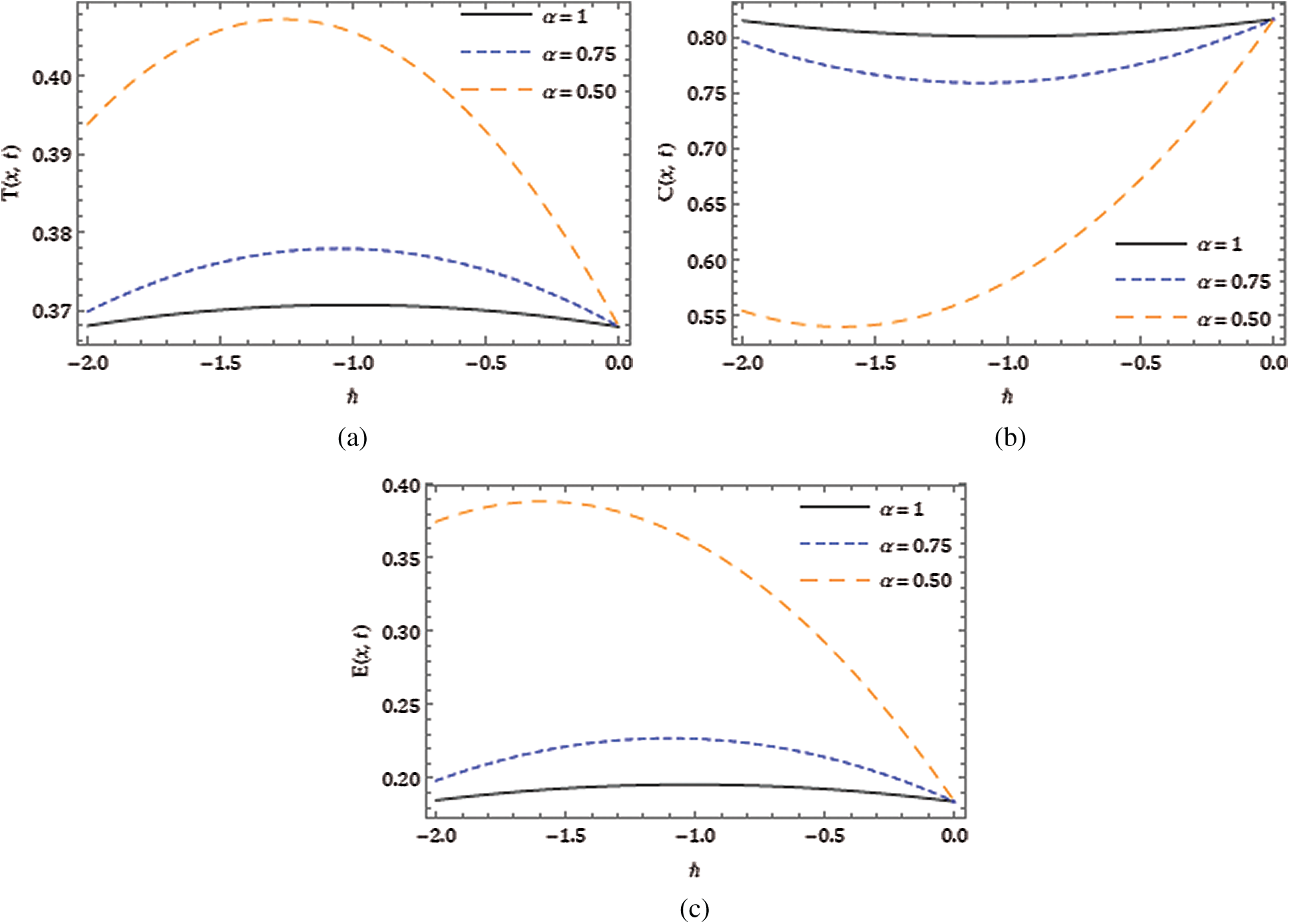
Figure 4:
The behaviors have been captured for different fractional Brownian motions and standard motion
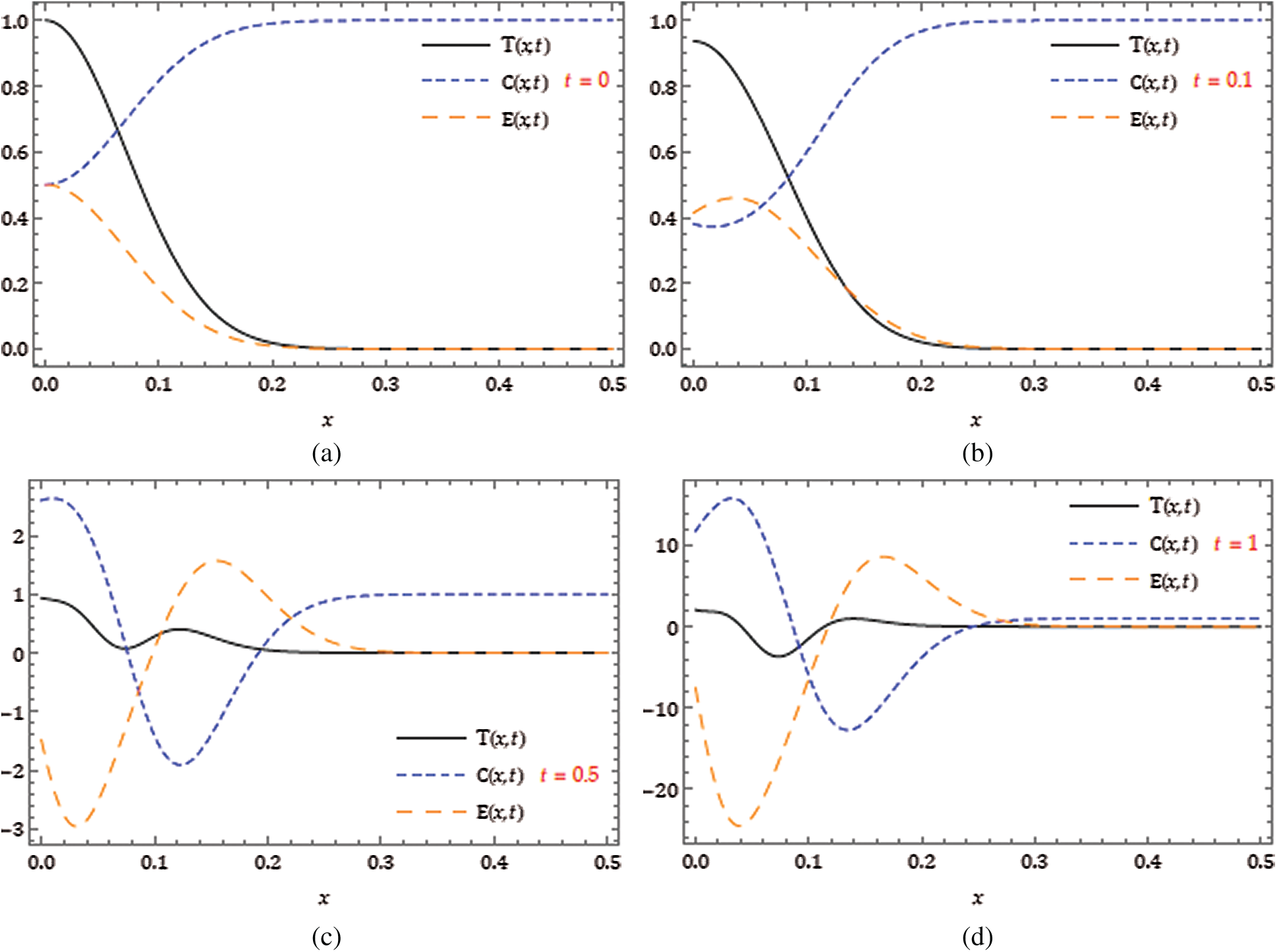
Figure 5: Response of obtained solution for the considered model with varying in
In the present study, we analyzed and capture the behaviour of the nonlinear fractional model of tumour invasion and metastasis by using the fractional operator and efficient analytical technique. The existences and uniqueness are demonstrated with the assist of a fixed point hypothesis. The plots captured in the present investigation display the stimulating behaviour and these can help scholars for some essential and interesting consequence of the hired system. The present study shows, the phenomena conspicuously be contingent on the time history and the time instant and, these can be proficiently studied using fundamental perceptions of FC and newly proposed fractional operator. The investigations of these types of models can provide new notions to analyze more real-world problems and it opens the door for employing an efficient method to study complex phenomena associated with science and technology.
Funding Statement: The authors received no specific funding for this study.
Conflicts of Interest: The authors declare that they have no conflicts of interest to report regarding the present study.
1. American Cancer Society (2012). Cancer facts and figures 2012. Atlanta: American Cancer Society. [Google Scholar]
2. Chaplain, M. A. J., Stuart, A. M. (1993). A model mechanism for the chemotactic response of endothelial cells to tumour angiogenesis factor. Mathematical Medicine and Biology: A Journal of the IMA, 10(3), 149–168. DOI 10.1093/imammb/10.3.149. [Google Scholar] [CrossRef]
3. Sherratt, J. A., Nowak, M. A. (1992). Oncogenes, anti-oncogenes and the immune response to cancer: A mathematical model. Proceedings of the Royal Society of London B, 248(1323), 261–271. DOI 10.1098/rspb.1992.0071. [Google Scholar] [CrossRef]
4. Gatenby, R. A., Gawlinski, E. T. (1996). A reaction-diffusion model of cancer invasion. Cancer Research, 56(24), 5745–5753. [Google Scholar]
5. Anderson, A. R. A., Chaplain, M. A. J. (1998). Continuous and discrete mathematical models of tumor-induced angiogenesis. Bulletin of Mathematical Biology, 60(5), 857–899. DOI 10.1006/bulm.1998.0042. [Google Scholar] [CrossRef]
6. Riemann, G. F. B. (1896). Versucheinerallgemeinen auffassung der integration und differentiation. Gesammelte mathematische werke. Leipzig, Germany: Druck und Verlag. [Google Scholar]
7. Caputo, M. (1969). Elasticita e dissipazione. Zanichelli, Bologna, Italy. [Google Scholar]
8. Miller, K. S., Ross, B. (1993). An introduction to fractional calculus and fractional differential equations. New York: A Wiley. [Google Scholar]
9. Podlubny, I. (1999). Fractional differential equations. New York: Academic Press. [Google Scholar]
10. Kilbas, A. A., Srivastava, H. M., Trujillo, J. J. (2006). Theory and applications of fractional differential equations. Amsterdam: Elsevier. [Google Scholar]
11. Ionescu, C., Lopes, A., Copot, D., Machado, J. A. T., Bates, J. H. T. (2017). The role of fractional calculus in modeling biological phenomena. Communications in Nonlinear Science and Numerical Simulation, 51, 141–159. DOI 10.1016/j.cnsns.2017.04.001. [Google Scholar] [CrossRef]
12. Veeresha, P., Prakasha, D. G., Baskonus, H. M. (2019). New numerical surfaces to the mathematical model of cancer chemotherapy effect in caputo fractional derivatives. Chaos, 29, 13119. DOI 10.1063/1.5074099. [Google Scholar] [CrossRef]
13. Yang, X. J., Baleanu, D., Khan, Y., Mohyud-Din, S. T. (2013). Local fractional variational iteration method for diffusion and wave equations on cantor set. Romanian Journal of Physics, 59(1–2), 36–48. [Google Scholar]
Veeresha, P., Baskonus, H. M. (2021). A powerful iterative approach for quintic complex Ginzburg–Landau equation within the frame of fractional operator. Fractals. Singapore: World Scientific. DOI 10.1142/S0218348X21400235. [Google Scholar] [CrossRef]
15. Merdan, M., Gökdoğan, A., Yıldırım, A., Mohyud-Din, S. T. (2012). Numerical simulation of fractional Fornberg–Whitham equation by differential transformation method. Abstract and Applied Analysis, 1–8. DOI 10.1155/2012/965367. [Google Scholar] [CrossRef]
16. Prakasha, D. G., Malagi, N. S., Veeresha, P., Prasannakumara, B. C. (2021). An efficient computational technique for time-fractional Kaup–Kupershmidt equation. Numerical Methods for Partial Differential Equations, 37(2), 1299–1316. DOI 10.1002/num.22580. [Google Scholar] [CrossRef]
17. Jain, R., Arekar, K., Dubey, R. S. (2017). Study of Bergman’s minimal blood glucose-insulin model by Adomian decomposition method. Journal of Information and Optimization Sciences, 38(1), 133–149. DOI 10.1080/02522667.2016.1187919. [Google Scholar] [CrossRef]
18. Meral, G., Yamanlar, I. C. (2018). Mathematical analysis and numerical simulations for the cancer tissue invasion model. Communications Faculty of Sciences University of Ankara Series A1 Mathematics and Statistics, 68, 371–391. DOI 10.31801/cfsuasmas.421546. [Google Scholar] [CrossRef]
19. Usha, S., Abinaya, V., Loghambal, S., Rajendran, L. (2012). Non-linear mathematical model of the interaction between tumor and on colytic viruses. Applied Mathematics, 3(9), 1089–1096. DOI 10.4236/am.2012.39160. [Google Scholar] [CrossRef]
20. Sun, H. G., Zhang, Y., Baleanu, D., Chen, W., Chen, Y. Q. (2018). A new collection of real world applications of fractional calculus in science and engineering. Communications in Nonlinear Science and Numerical Simulation, 64(48103), 213–231. DOI 10.1016/j.cnsns.2018.04.019. [Google Scholar] [CrossRef]
21. Atangana, A., Baleanu, D. (2016). New fractional derivatives with non-local and non-singular kernel theory and application to heat transfer model. Thermal Science, 20(2), 763–769. DOI 10.2298/TSCI160111018A. [Google Scholar] [CrossRef]
22. Veeresha, P., Prakasha, D. G., Baskonus, H. M. (2019). Novel simulations to the time-fractional Fisher’s equation. Mathematical Sciences, 13(1), 33–42. DOI 10.1007/s40096-019-0276-6. [Google Scholar] [CrossRef]
23. Veeresha, P., Prakasha, D. G. (2021). Solution for fractional Kuramoto–Sivashinsky equation using novel computational technique. International Journal of Applied and Computational Mathematics, 7(2), 1. DOI 10.1007/s40819-021-00956-0. [Google Scholar] [CrossRef]
24. Prakash, A., Veeresha, P., Prakasha, D. G., Goyal, M. (2019). A homotopy technique for fractional order multi-dimensional telegraph equation via Laplace transform. The European Physical Journal Plus, 134(1), 3698. DOI 10.1140/epjp/i2019-12411-y. [Google Scholar] [CrossRef]
25. Veeresha, P., Prakasha, D. G. (2020). An efficient technique for two-dimensional fractional order biological population model. International Journal of Modeling, Simulation, and Scientific Computing, 11(1), 2050005. DOI 10.1142/S1793962320500051. [Google Scholar] [CrossRef]
26. Atangana, A., Alkahtani, B. T. (2015). Analysis of the Keller–Segel model with a fractional derivative without singular kernel. Entropy, 17(12), 4439–4453. DOI 10.3390/e17064439. [Google Scholar] [CrossRef]
27. Atangana, A., Alkahtani, B. T. (2016). Analysis of non-homogenous heat model with new trend of derivative with fractional order. Chaos Solitons Fractals, 89(273), 566–571. DOI 10.1016/j.chaos.2016.02.012. [Google Scholar] [CrossRef]
28. Panda, S. K., Abdeljawad, T., Ravichandran, C. (2020). A complex valued approach to the solutions of Riemann–Liouville integral, Atangana–Baleanu integral operator and non-linear telegraph equation via fixed point method. Chaos Solitons Fractals, 130(2), 109439. DOI 10.1016/j.chaos.2019.109439. [Google Scholar] [CrossRef]
29. Belmor, S., Ravichandran, C., Jarad, F. (2020). Nonlinear generalized fractional differential equations with generalized fractional integral conditions. Journal of Taibah University for Science, 14(1), 114–123. DOI 10.1080/16583655.2019.1709265. [Google Scholar] [CrossRef]
30. Gao, W., Veeresha, P., Baskonus, H. M., Prakasha, D. G., Kumar, P. (2020). A new study of unreported cases of 2019-nCOV epidemic outbreaks. Chaos Solitons Fractals, 138(554), 109929. DOI 10.1016/j.chaos.2020.109929. [Google Scholar] [CrossRef]
31. Valliammal, N., Ravichandran, C., Nisar, K. S. (2020). Solutions to fractional neutral delay differential nonlocal systems. Chaos Solitons Fractals, 138(1), 109912. DOI 10.1016/j.chaos.2020.109912. [Google Scholar] [CrossRef]
32. Veeresha, P., Prakasha, D. G., Singh, J., Khan, I., Kumar, D. (2020). Analytical approach for fractional extended Fisher–Kolmogorov equation with Mittag-Leffler kernel. Advances in Difference Equations, 174. DOI 10.1186/s13662–020-02617-w. [Google Scholar] [CrossRef]
33. Caputo, M., Fabrizio, M. (2015). A new definition of fractional derivative without singular kernel. Progress in Fractional Differentiation and Applications, 1(2), 73–85. DOI 10.12785/pfda/010201. [Google Scholar] [CrossRef]
34. Baishya, C. (2020). Dynamics of fractional stage structured predator prey model with prey refuge. Indian Journal of Ecology, 47(4), 1118–1124. [Google Scholar]
35. Baba, I. A., Nasidi, B. A. (2020). Fractional order model for the role of mild cases in the transmission of COVID-19. Chaos Solitons Fractals, 142, 110374. DOI 10.1016/j.chaos.2020.110374. [Google Scholar] [CrossRef]
36. Ahmed, I., Baba, I. A., Yusuf, A., Kumam, P., Kumam, W. (2020). Analysis of Caputo fractional-order model for COVID-19 with lockdown. Advances in Difference Equations, 394(1), 119. DOI 10.1186/s13662-020-02853-0. [Google Scholar] [CrossRef]
37. Baba, I. A., Nasidi, B. A. (2021). Fractional order epidemic model for the dynamics of novel COVID-19. Alexandria Engineering Journal, 60(1), 537–548. DOI 10.1016/j.aej.2020.09.029. [Google Scholar] [CrossRef]
38. Baba, I. A., Baba, B. A., Esmaili, P. (2020). A mathematical model to study the effectiveness of some of the strategies adopted in curtailing the spread of COVID-19. Computational and Mathematical Methods in Medicine, 2020(1), 1–6. DOI 10.1155/2020/5248569. [Google Scholar] [CrossRef]
39. Baba, I. A., Baleanu, D. (2020). Awareness as the most effective measure to mitigate the spread of COVID-19 in Nigeria. Computers, Materials & Continua, 65(3), 1945–1957. DOI 10.32604/cmc.2020.011508. [Google Scholar] [CrossRef]
40. Rezapour, S., Mohammadi, H., Jajarmi, A. (2020). A new mathematical model for Zika virus transmission. Advances in Difference Equations, 589(2020), 479. DOI 10.1186/s13662-020-03044-7. [Google Scholar] [CrossRef]
41. Baleanu, D., Ghanbari, B., Asad, J. H., Jajarmi, A., Pirouz, H. M. (2020). Planar system-masses in an equilateral triangle: Numerical study within fractional calculus. Computer Modeling in Engineering & Sciences, 124(3), 953–968. DOI 10.32604/cmes.2020.010236. [Google Scholar] [CrossRef]
42. Baleanu, D., Jajarmi, A., Sajjadi, S. S., Asad, J. H. (2020). The fractional features of a harmonic oscillator with position-dependent mass. Communications in Theoretical Physics, 72(5), 055002. DOI 10.1088/1572-9494/ab7700. [Google Scholar] [CrossRef]
43. Akram, T. (2020). An efficient numerical technique for solving time fractional Burgers equation. Alexandria Engineering Journal, 59(4), 2201–2220. DOI 10.1016/j.aej.2020.01.048. [Google Scholar] [CrossRef]
44. Jajarmi, A., Baleanu, D. (2019). On the fractional optimal control problems with a general derivative operator. Asian Journal of Control, 23(2), 1062–1071. DOI 10.1002/asjc.2282. [Google Scholar] [CrossRef]
45. Iqbal, M. K., Abbas, M., Wasim, I. (2018). New cubic B-spline approximation for solving third order Emden–Flower type equations. Applied Mathematics and Computation, 331(1), 319–333. DOI 10.1016/j.amc.2018.03.025. [Google Scholar] [CrossRef]
46. Khalid, N., Abbas, M., Iqbal, M. K., Singh, J., Ismail, A. I. M. (2020). A computational approach for solving time fractional differential equation via spline functions. Alexandria Engineering Journal, 59(5), 3061–3078. DOI 10.1016/j.aej.2020.06.007. [Google Scholar] [CrossRef]
47. Sajjadia, S. S., Baleanu, D., Jajarmi, A., Pirouz, H. M. (2020). A new adaptive synchronization and hyper chaos control of a biological snap oscillator. Chaos Solitons Fractals, 138, 109919. DOI 10.1016/j.chaos.2020.109919. [Google Scholar] [CrossRef]
48. Gao, W., Veeresha, P., Prakasha, D. G., Baskonus, H. M. (2020). New numerical simulation for fractional Benney–Lin equation arising in falling film problems using two novel techniques. Numerical Methods for Partial Differential Equations, 37(1), 210–243. DOI 10.1002/num.22526. [Google Scholar] [CrossRef]
49. Baishya, C. (2019). A new application of hermite collocation method. International Journal of Mathematical, Engineering and Management Sciences, 4(1), 182–190. DOI 10.33889/24557749. [Google Scholar] [CrossRef]
50. Jajarmi, A., Baleanu, D. (2020). A new iterative method for the numerical solution of high-order nonlinear fractional boundary value problems. Frontiers in Physics, 8(220), 545. DOI 10.3389/fphy.2020.00220. [Google Scholar] [CrossRef]
51. Khalid, N., Abbas, M., Iqbal, M. K. (2019). Non-polynomial quintic spline for solving fourth-order fractional boundary value problems involving product terms. Applied Mathematics and Computation, 349(1), 393–407. DOI 10.1016/j.amc.2018.12.066. [Google Scholar] [CrossRef]
52. Gao, W., Veeresha, P., Prakasha, D. G., Baskonus, H. M., Yel, G. (2020). New approach for the model describing the deathly disease in pregnant women using Mittag–Leffler function. Chaos Solitons Fractals, 134, 109696. DOI 10.1016/j.chaos.2020.109696. [Google Scholar] [CrossRef]
53. Owusu-Mensah, I., Akinyemi, L., Oduro, B., Iyiola, O. S. (2020). A fractional order approach to modeling and simulations of the novel COVID-19. Advances in Difference Equations, 683(1), 211. DOI 10.1186/s13662-020-03141-7. [Google Scholar] [CrossRef]
54. Liao, S. J. (1997). Homotopy analysis method and its applications in mathematics. Journal of Basic Science and Engineering, 5(2), 111–125. [Google Scholar]
55. Singh, J., Kumar, D., Swroop, R. (2016). Numerical solution of time-and space-fractional coupled Burgers’ equations via homotopy algorithm. Alexandria Engineering Journal, 55(2), 1753–1763. DOI 10.1016/j.aej.2016.03.028. [Google Scholar] [CrossRef]
56. Prakasha, D. G., Veeresha, P. (2020). Analysis of Lakes pollution model with Mittag–Leffler kernel. Journal of Ocean Engineering and Science, 5(4), 310–322. DOI 10.1016/j.joes.2020.01.004. [Google Scholar] [CrossRef]
57. Srivastava, H. M., Kumar, D., Singh, J. (2017). An efficient analytical technique for fractional model of vibration equation. Applied Mathematical Modelling, 45(3), 192–204. DOI 10.1016/j.apm.2016.12.008. [Google Scholar] [CrossRef]
58. Veeresha, P., Prakasha, D. G., Baleanu, D. (2020). Analysis of fractional Swift-Hohenberg equation using a novel computational technique. Mathematical Methods in the Applied Sciences, 43(4), 1970–1987. DOI 10.1002/mma.6022. [Google Scholar] [CrossRef]
59. Veeresha, P., Prakasha, D. G. (2020). A reliable analytical technique for fractional Caudrey–Dodd–Gibbon equation with Mittag–Leffler kernel. Nonlinear Engineering, 9(1), 319–328. DOI 10.1515/nleng-2020-0018. [Google Scholar] [CrossRef]
60. Kumar, D., Agarwal, R. P., Singh, J. (2018). A modified numerical scheme and convergence analysis for fractional model of Lienard’s equation. Journal of Computational and Applied Mathematics, 399(1), 405–413. DOI 10.1016/j.cam.2017.03.011. [Google Scholar] [CrossRef]
61. Veeresha, P., Prakasha, D. G. (2019). Solution for fractional Zakharov–Kuznetsov equations by using two reliable techniques. Chinese Journal of Physics, 60(1), 313–330. DOI 10.1016/j.cjph.2019.05.009. [Google Scholar] [CrossRef]
62. Safare, K. M., Betageri, V. S., Prakasha, D. G., Veeresha, P., Kumar, S. (2021). A mathematical analysis of ongoing outbreak COVID-19 in India through nonsingular derivative. Numerical Methods for Partial Differential Equations, 37(2), 1282–1298. DOI 10.1002/num.22579. [Google Scholar] [CrossRef]
63. Veeresha, P., Prakasha, D. G., Kumar, S. (2020). A fractional model for propagation of classical optical solitons by using non-singular derivative. Mathematical Methodsin the Applied Sciences, 75(4), 125. DOI 10.1002/mma.6335. [Google Scholar] [CrossRef]
64. Gao, W., Baskonus, H. M., Shi, L. (2020). New investigation of bats-hosts-reservoir-people coronavirus model and apply to 2019-nCoV system. Advances in Difference Equations, 2020(391), 1–11. DOI 10.1186/s13662-019-2438-0. [Google Scholar] [CrossRef]
65. Al-Ghafri, K. S., Rezazadeh, H. (2019). Solitons and other solutions of (3 + 1)-dimensional space-time fractional modified KdV–Zakharov–Kuznetsov equation. Applied Mathematics and Nonlinear Sciences, 4(2), 289–304. DOI 10.2478/AMNS.2019.2.00026. [Google Scholar] [CrossRef]
66. Durur, H., Ilhan, E., Bulut, H. (2020). Novel complex wave solutions of the (2 + 1)-dimensional hyperbolic nonlinear schrödinger equation. Fractal and Fractional, 4(3), 41. DOI 10.3390/fractalfract4030041. [Google Scholar] [CrossRef]
67. Ilhan, E., Kıymaz, I. O. (2020). A generalization of truncated M-fractional derivative and applications to fractional differential equations. Applied Mathematics and Nonlinear Sciences, 5(1), 171–188. DOI 10.2478/amns.2020.1.00016. [Google Scholar] [CrossRef]
68. Gao, W., Veeresha, P., Prakasha, D. G., Baskonus, H. M. (2020). Novel dynamical structures of 2019-nCoV with nonlocal operator via powerful computational technique. Biology, 9(5), 107. DOI 10.3390/biology9050107. [Google Scholar] [CrossRef]
69. Yokus, A., Gulbahar, S. (2019). Numerical solutions with linearization techniques of the fractional harry dym equation. Applied Mathematics and Nonlinear Sciences, 4(1), 35–42. DOI 10.2478/AMNS.2019.1.00004. [Google Scholar] [CrossRef]
70. Gao, W., Veeresha, P., Prakasha, D. G., Baskonus, H. M., Gulnur, Y. (2020). New numerical results for the time-fractional Phi-four equation using a novel analytical approach. Symmetry, 12(478), 1–16. DOI 10.3390/sym12030478. [Google Scholar] [CrossRef]
71. Brzeziński, D. W. (2018). Review of numerical methods for NumILPT with computational accuracy assessment for fractional calculus. Applied Mathematics and Nonlinear Sciences, 3(2), 487–502. DOI 10.2478/AMNS.2018.2.00038. [Google Scholar] [CrossRef]
72. Gao, W., Gulnur, Y., Baskonus, H. M., Cattani, C. (2020). Complex solitons in the conformable (2 + 1)-dimensional Ablowitz-Kaup–Newell–Segur equation. AIMS Math, 5(1), 507–521. DOI 10.3934/math.2020034. [Google Scholar] [CrossRef]
73. Losada, J., Nieto, J. J. (2015). Properties of the new fractional derivative without singular Kernel. Progress in Fractional Differentiation and Applications, 1, 87–92. DOI 10.12785/pfda/010202. [Google Scholar] [CrossRef]
74. Anderson, A. R. A., Chaplain, M. A. J., Newman, E. L., Steeele, R. J. C., Thompson, A. M. (2000). Mathematical modelling of tumour invasion and metastasis. Computational and Mathematical Methods in Medicine, 2(2), 129–154. DOI 10.1080/10273660008833042. [Google Scholar] [CrossRef]
75. Stetler-Stevenson, W. G., Hewitt, R., Corcoran, M. (1996). Matrix metallo-proteinases and tumour invasion, from correlation to causality to the clinic. Cancer Biology, 7(3), 147–154. DOI 10.1006/scbi.1996.0020. [Google Scholar] [CrossRef]
76. Chambers, A. F., Matrisian, L. M. (1997). Changing views of the role of matrix metalloproteinases in metastasis. Journal of the National Cancer Institute, 89(17), 1260–1270. DOI 10.1093/jnci/89.17.1260. [Google Scholar] [CrossRef]
77. Mahiddin, N., Ali, S. A. H. (2014). Approximate analytical solutions for mathematical model of tumour invasion and metastasis using modified Adomian decomposition and homotopy perturbation methods. Journal of Applied Mathematics, 1–13. DOI 10.1155/2014/654978. [Google Scholar] [CrossRef]
 | This work is licensed under a Creative Commons Attribution 4.0 International License, which permits unrestricted use, distribution, and reproduction in any medium, provided the original work is properly cited. |