| Computer Modeling in Engineering & Sciences |
DOI: 10.32604/cmes.2021.015310
ARTICLE
A Pseudo-Spectral Scheme for Systems of Two-Point Boundary Value Problems with Left and Right Sided Fractional Derivatives and Related Integral Equations
1Department of Mathematics, Faculty of Science, Al-Azhar University, Cairo, Egypt
2Department of Mathematics, Faculty of Science, Cairo University, Giza, 12613, Egypt
3Department of Applied Mathematics, Physics Division, National Research Centre, Dokki, Cairo, 12622, Egypt
4Department of Computational Mathematics and Computer Science, Institute of Natural Sciences and Mathematics, Ural Federal University, Yekaterinburg, 620002, Russia
5Department of Mathematics, Faculty of Science, Benha University, Benha, 13511, Egypt
*Corresponding Author: M. A. Zaky. Email: ma.zaky@yahoo.com; zaky.nrc@gmail.com
Received: 08 December 2020; Accepted: 04 March 2021
Abstract: We target here to solve numerically a class of nonlinear fractional two-point boundary value problems involving left- and right-sided fractional derivatives. The main ingredient of the proposed method is to recast the problem into an equivalent system of weakly singular integral equations. Then, a Legendre-based spectral collocation method is developed for solving the transformed system. Therefore, we can make good use of the advantages of the Gauss quadrature rule. We present the construction and analysis of the collocation method. These results can be indirectly applied to solve fractional optimal control problems by considering the corresponding Euler–Lagrange equations. Two numerical examples are given to confirm the convergence analysis and robustness of the scheme.
Keywords: Spectral collocation method; weakly singular integral equations; two-point boundary value problems; convergence analysis
Fractional-order differential operators have recently risen to prominence in the modelling of several processes. The mathematical models involving these operators have also attracted much attention, a survey of recent activity is given in [1–3]. The issue we address in this paper is to construct and analyse a spectral collocation method to solve the following nonlinear system of Caputo fractional two-point boundary value problems:
where fR and
Because the fractional-order differential operators are nonlocal with weakly singular kernels, the numerical discretization of the fractional models is more change than the classical schemes. There are several analytical schemes to solve fractional differential equations, such as the Green’s function method, the Mellin transform method, the Laplace transform method, the Fourier transform method, and so on [4–7]. However, analytical methods are rare for most of fractional differential equations, e.g., with non linearities or linear equations with time-dependent coefficients. Hence, constructing efficient numerical approaches is of great importance in practical applications.
Many numerical schemes have been developed to solve the fractional differential equations, mostly with the finite element methods (e.g., [8–11] and the references therein) and the finite difference methods (e.g., [12–18] and the references therein). Since spectral methods are capable of providing high-order accurate numerical approximations with less degrees of freedoms [19–23], they have been widely used for numerical approximations of fractional differential equations [24–29] or its related integral equations [30–37]. In particular, well designed spectral methods appear to be particularly attractive to tackle the difficulties associated with the weakly singular kernels of the fractional differential operators and the integral equations [38,39].
The system of fractional two-point boundary value problems (1) can be converted to an equivalent weakly singular nonlinear system of Volterra integral equations (15). The key idea of the presented approach is to solve (15) using the Legendre spectral collocation scheme. The aim of that convert to (15) is to approximate the related integral terms by the Gauss quadrature formula. The presented method has spectral convergence. This theoretical estimate is confirmed by two numerical test examples. Specifically, our strategies and contributions are highlighted as follows:
i) The system of fractional two-point boundary value problems is recast into an equivalent weakly singular nonlinear system of Volterra integral equations.
ii) The Legendre spectral collocation method is applied to the transformed equation.
iii) The convergence analysis of the Legendre collocation method under the L2-norms is derived.
The structure of the paper is as follows. In Section 2, we introduce some necessary definitions, notations and lemmas. The Legendre spectral collocation scheme is presented in Section 3. The convergence analysis is provided in Section 4. In Section 5, numerical examples are performed to confirm the efficiency of the numerical method. A brief conclusion is highlighted in Section 6.
In this section, we provide some notations, definitions, and some useful lemmas about the fractional differential and integral operators [4] and the Jacobi polynomials.
Definition 1. Let
where
Definition 2. The left- and right-sided Caputo fractional derivatives are defined as:
where ,
Definition 3. The left- and right-sided Riemann-Liouville fractional derivatives are defined as:
It is worthy to mention here that the left- and right-sided Caputo fractional derivatives satisfy the following fundamental properties
Theorem 1. There hold [4]
where
The following formulas introduce the relationship between the Riemann-Liouville and the Caputo fractional derivatives [5].
Let
and for
Now, we give some basic properties of the Jacobi polynomials and related Jacobi–Gauss interpolation. For
where,
Denote
The formula (11) is exact for any
For any
The above condition indicates that
The Legendere polynomials can be obtained directly from the properties of the Jacobi polynomials by setting
We consider the system of two-point fractional boundary value problems (1) with homogeneous boundary conditions. There is no loss of generality since this can always be accomplished by a simple change of variables.
The above system is equivalent to the following system of weakly singular integral equations:
The variable transformations
The Legendre spectral collocation scheme for (17) and (18) is to seek uN(x) and
We now describe the implementation procedure of (19), (20) in detail. We consider the following Legendre approximations
and
Then, by (21) and (9) direct computations lead to
Applying (12) to (21), one can verify readily that
Similarly
Hence, by using (17)–(26) we deduce that
Finally, using (9) we obtain
This system of equations can be solved for
In this section, we introduce some functional spaces. We denote
Definition 4. Let
with the inner product and norm
Definition 5. For a non-negative integer s. The weighted Jacobi non-uniformly Sobolev space
with the inner product, norm, and semi-norm
In particular,
The space
Lemma 1. (cf. [40]) Let
where
Lemma 2. (cf. [40]) For any
Lemma 3. (cf. [41]) Let
Let
Hence
and
It is not difficult to obtain the following results
Similarly
We denote
Let
Hence,
and
We can also derive the following results
Similarly
and
In this section, we analyze the numerical errors of the systems (19) and (20). Let E = |Eu|+|Ev|, where Eu = u − uN, Ev = v − vN and denote by
Lemma 4. The following inequality holds
where
Proof. It follows from (16) and (46) that
Subtracting (57) from (56) yields
Similarly, from (16) and (52) we deduce that
Subtracting (60) from (59) yields
and adding (58) and (61) yields
The above equation can be rewritten as
The desired result follows immediately from the above.
Throughout this section, we suppose that fL and fR fulfil the Lipschitz conditions
with the Lipschitz positive constants L11 and L22, are chosen such that
Theorem 2. Let uN(x) and vN(x) be the solutions of the systems of Eqs. (17) and (18), respectively,
Proof. Using Lemma (4), we get
and
We now estimate
using the Cauchy-Schwarz inequality, we further get
making use of (48) leads to
Using similar arguments leads to
We now estimate
Using (47), we obtain
Using (46) and the Lipschitz condition, we get
For
hence,
Similarly, we can deduce that
Using the condition (65) and knowing that
In this section, two numerical examples are provided to illustrate the efficiency and applicability of the proposed method.
Example 1. We consider the following system of fractional differential equations:
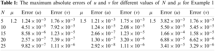
The boundary conditions are chosen such that the exact solution is given by u(z) = (1+z)3.5 and v(z) = (1 − z)2.5. In Figs. 1 and 2 we list the L2-error of the approximate solutions uN and vN, respectively, in log scale against various N and
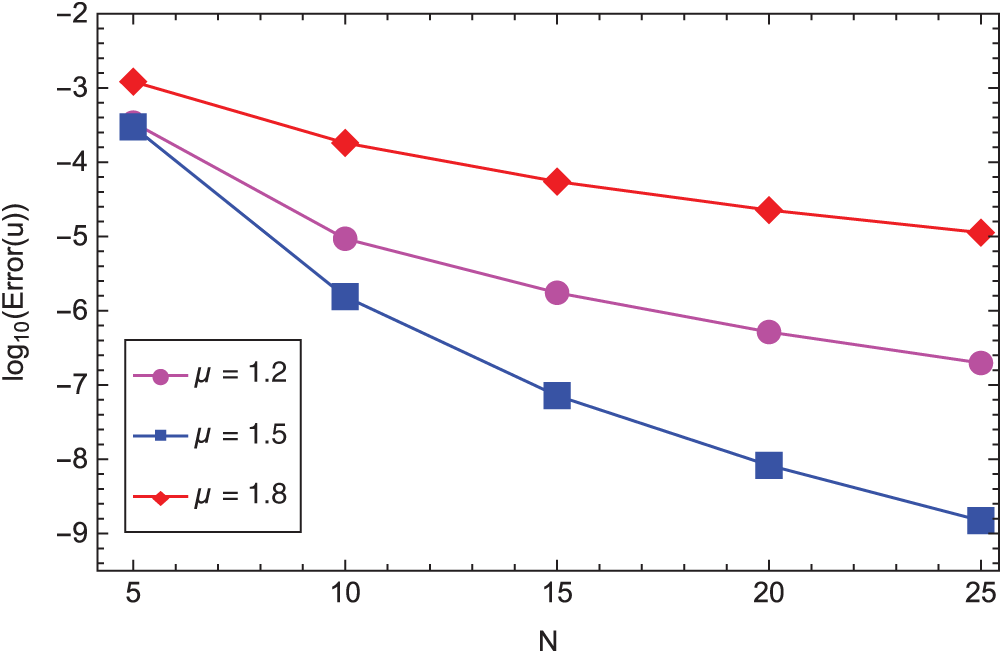
Figure 1: The L2-error of the approximate solution uN in log scale vs. various N and
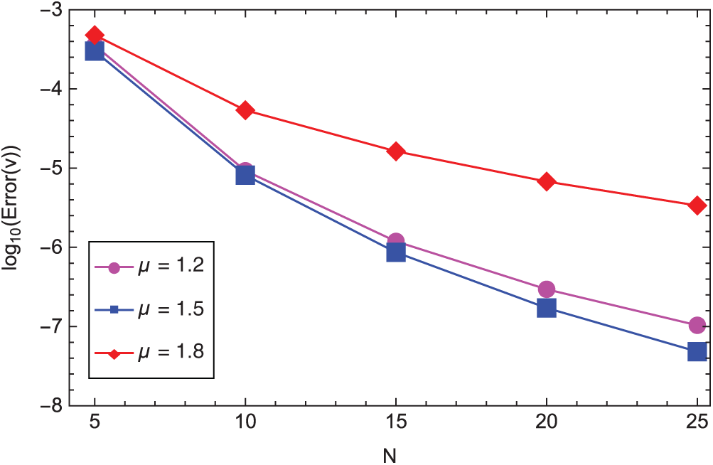
Figure 2: The L2-error of the approximate solution vN in log scale vs. various N and
Example 2. We consider the following system of fractional differential equations: [28]:
In Tab. 2, we compare our results with those reported in [42]. These results indicate that the proposed spectral method is more accurate than the Ritz method [42]. In Tab. 3, we list the maximum absolute errors for different values of N and
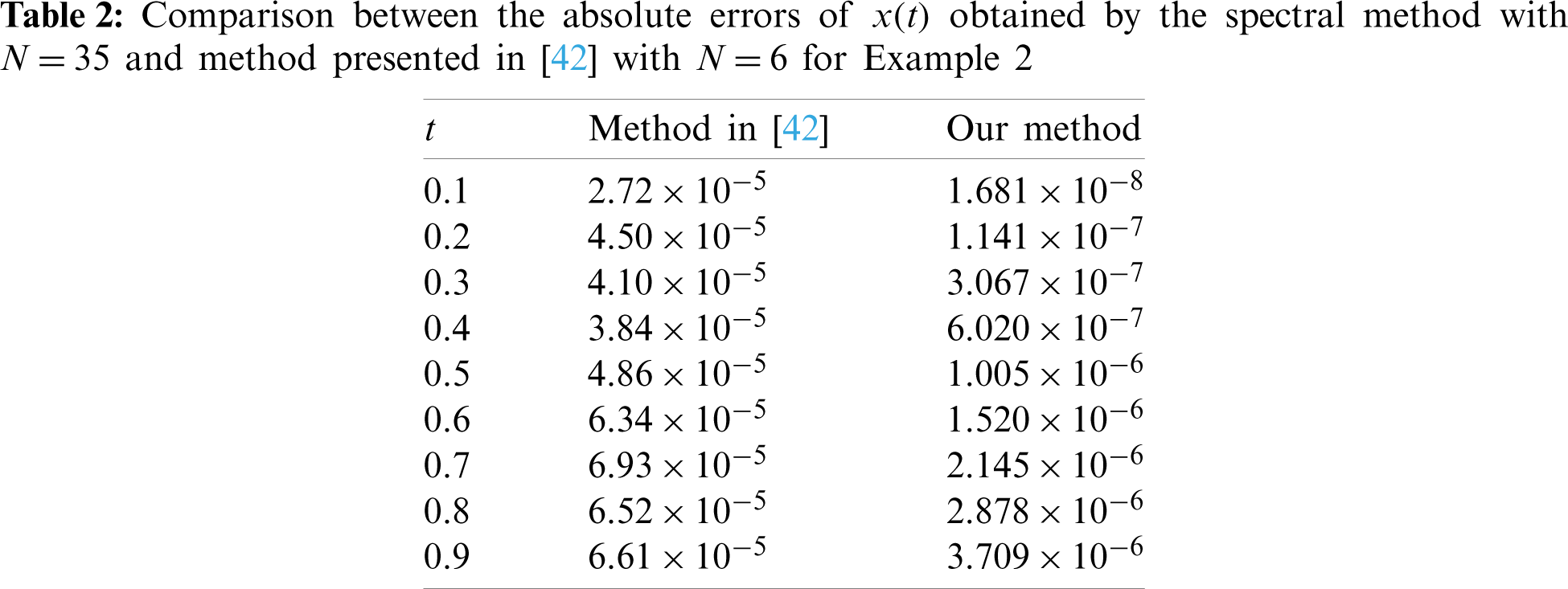
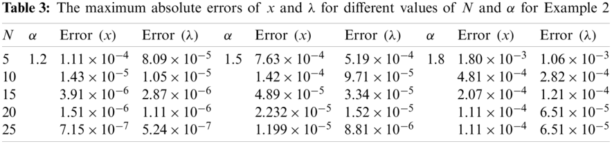
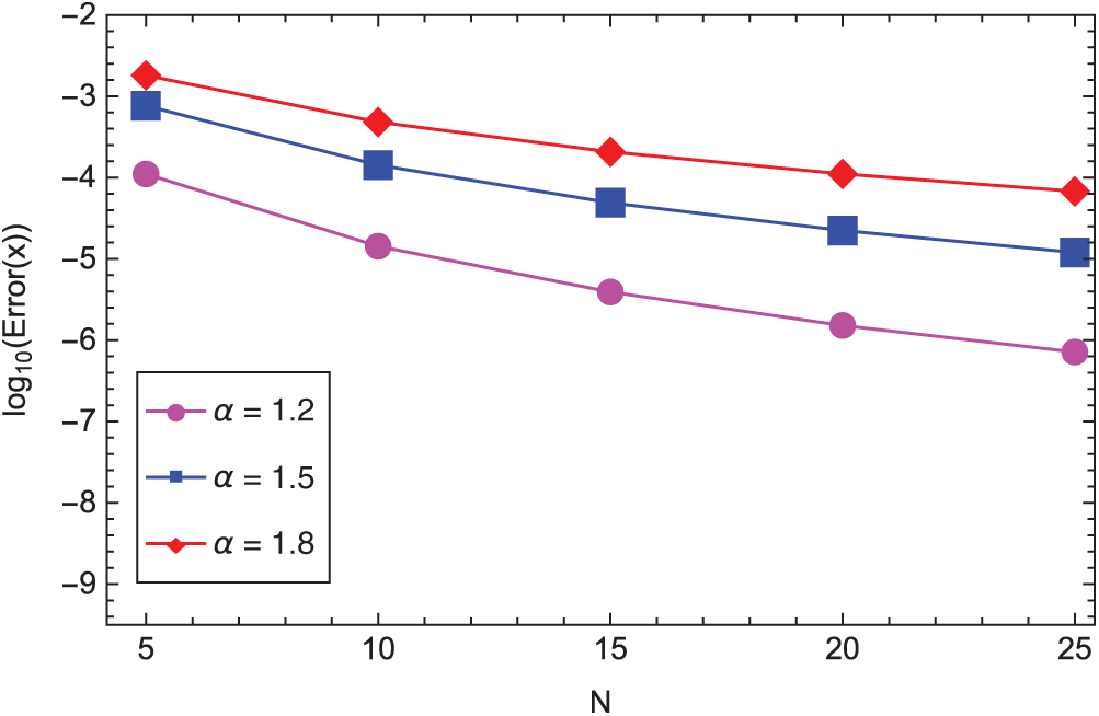
Figure 3: The
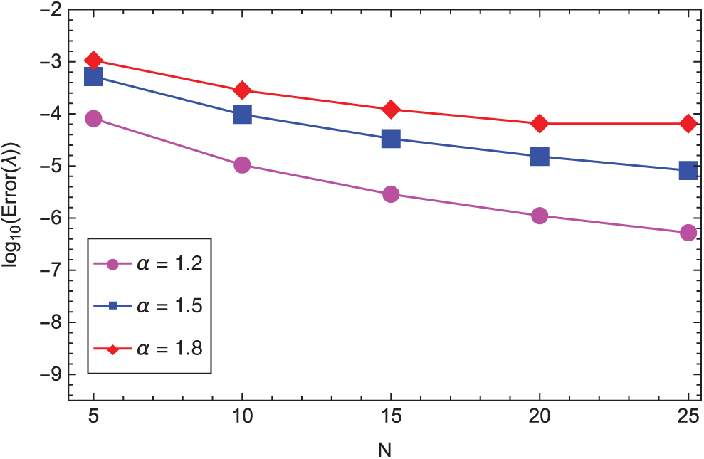
Figure 4: The
Numerically solving a class of nonlinear fractional two-point boundary value problems involving left- and right-sided fractional derivatives was fulfilled as a target of that work. The way to achieve that was done indirectly by recasting the considered system into a weakly singular integral system for the sake of the possibility of applying the Gauss quadrature rule on the transformed integral system. The construction and analysis of the used collocation method is proposed. The obtained results can be indirectly applied to solve fractional optimal control problems by considering the corresponding Euler–Lagrange equations [43,44]. A numerical example was given to confirm the convergence analysis and robustness of the scheme. Our future work is related to spectral methods for systems of nonlinear fractional differential equations and system of integral equations with non-smooth solutions.
Funding Statement: The Russian Foundation for Basic Research (RFBR) Grant No. 19-01-00019.
Conflicts of Interest: The authors declare that they have no conflicts of interest to report regarding the present study.
1. Machado, J. T., Kiryakova, V., Mainardi, F. (2011). Recent history of fractional calculus. Communications in Nonlinear Science and Numerical Simulation, 16(3), 1140–1153. DOI 10.1016/j.cnsns.2010.05.027. [Google Scholar] [CrossRef]
2. Tarasov, V. E. (2019). On history of mathematical economics: Application of fractional calculus. Mathematics, 7(6), 509. DOI 10.3390/math7060509. [Google Scholar] [CrossRef]
3. Sun, H., Zhang, Y., Baleanu, D., Chen, W., Chen, Y. (2018). A new collection of real world applications of fractional calculus in science and engineering. Communications in Nonlinear Science and Numerical Simulation, 64(48103), 213–231. DOI 10.1016/j.cnsns.2018.04.019. [Google Scholar] [CrossRef]
4. Podlubny, I. (1998). Fractional differential equations: An introduction to fractional derivatives, fractional differential equations, to methods of their solution and some of their applications. Amsterdam, Netherlands: Elsevier. [Google Scholar]
5. Nikan, O., Machado, J. T., Golbabai, A., Rashidinia, J. (2021). Numerical evaluation of the fractional Klein–Kramers model arising in molecular dynamics. Journal of Computational Physics, 428(1), 109983. DOI 10.1016/j.jcp.2020.109983. [Google Scholar] [CrossRef]
6. Diethelm, K. (2010). The analysis of fractional differential equations: An application-oriented exposition using differential operators of caputo type. Berlin, Germany: Springer Science & Business Media. [Google Scholar]
7. Hassani, H., Machado, J. T., Mehrabi, S. (2021). An optimization technique for solving a class of nonlinear fractional optimal control problems: Application in cancer treatment. Applied Mathematical Modelling, 93(3), 868–884. DOI 10.1016/j.apm.2021.01.004. [Google Scholar] [CrossRef]
8. Jin, B., Lazarov, R., Pasciak, J., Zhou, Z. (2014). Error analysis of a finite element method for the space-fractional parabolic equation. SIAM Journal on Numerical Analysis, 52(5), 2272–2294. DOI 10.1137/13093933X. [Google Scholar] [CrossRef]
9. Gao, X., Liu, F., Li, H., Liu, Y., Turner, I. et al. (2020). A novel finite element method for the distributed-order time fractional cable equation in two dimensions. Computers & Mathematics with Applications, 80(5), 923–939. DOI 10.1016/j.camwa.2020.04.019. [Google Scholar] [CrossRef]
10. Li, L., Liu, F., Feng, L., Turner, I. (2020). A Galerkin finite element method for the modified distributed-order anomalous sub-diffusion equation. Journal of Computational and Applied Mathematics, 368, 112589. DOI 10.1016/j.cam.2019.112589. [Google Scholar] [CrossRef]
11. Loghman, E., Kamali, A., Bakhtiari-Nejad, F., Abbaszadeh, M. (2021). Nonlinear free and forced vibrations of fractional modeled viscoelastic FGM micro-beam. Applied Mathematical Modelling, 92(4), 297–314. DOI 10.1016/j.apm.2020.11.011. [Google Scholar] [CrossRef]
12. Feng, L., Liu, F., Turner, I. (2019). Finite difference/finite element method for a novel 2D multi-term time-fractional mixed sub-diffusion and diffusion-wave equation on convex domains. Communications in Nonlinear Science and Numerical Simulation, 70(3), 354–371. DOI 10.1016/j.cnsns.2018.10.016. [Google Scholar] [CrossRef]
13. Gracia, J. L., Stynes, M. (2015). Central difference approximation of convection in Caputo fractional derivative two-point boundary value problems. Journal of Computational and Applied Mathematics, 273(3), 103–115. DOI 10.1016/j.cam.2014.05.025. [Google Scholar] [CrossRef]
14. Zaky, M. A., Hendy, A. S., Macas-Daz, J. E. (2020). High-order finite difference/spectral-Galerkin approximations for the nonlinear time–space fractional Ginzburg–Landau equation. Numerical Methods for Partial Differential Equations, 1–26. DOI 10.1002/num.22630. [Google Scholar] [CrossRef]
15. Stynes, M., Gracia, J. L. (2015). A finite difference method for a two-point boundary value problem with a Caputo fractional derivative. IMA Journal of Numerical Analysis, 35(2), 698–721. DOI 10.1093/imanum/dru011. [Google Scholar] [CrossRef]
16. Abbaszadeh, M., Dehghan, M. (2020). A POD-based reduced-order Crank-Nicolson/fourth-order alternating direction implicit (ADI) finite difference scheme for solving the two-dimensional distributed-order Riesz space-fractional diffusion equation. Applied Numerical Mathematics, 158(10), 271–291. DOI 10.1016/j.apnum.2020.07.020. [Google Scholar] [CrossRef]
17. Abbaszadeh, M., Dehghan, M. (2020). A finite-difference procedure to solve weakly singular integro partial differential equation with space-time fractional derivatives. Engineering with Computers, 1–10. DOI 10.1007/s00366-020-00936-w. [Google Scholar] [CrossRef]
18. Abbaszadeh, M., Dehghan, M. (2020). Fourth-order alternating direction implicit (ADI) difference scheme to simulate the space-time Riesz tempered fractional diffusion equation. International Journal of Computer Mathematics, 1–24. DOI 10.1080/00207160.2020.1841175. [Google Scholar] [CrossRef]
19. Abo-Gabal, H., Zaky, M. A., Hafez, R. M., Doha, E. H. (2020). On Romanovski–Jacobi polynomials and their related approximation results. Numerical Methods for Partial Differential Equations, 36(6), 1982–2017. DOI 10.1002/num.22513. [Google Scholar] [CrossRef]
20. Zaky, M. A., Hendy, A. S. (2021). An efficient dissipation-preserving Legendre–Galerkin spectral method for the Higgs Boson equation in the de Sitter spacetime universe. Applied Numerical Mathematics, 160(283), 281–295. DOI 10.1016/j.apnum.2020.10.013. [Google Scholar] [CrossRef]
21. Hafez, R. M., Zaky, M. A. (2019). High-order continuous Galerkin methods for multi-dimensional advection-reaction–diffusion problems. Engineering with Computers, 36(4), 1813–1829. DOI 10.1007/s00366-019-00797-y. [Google Scholar] [CrossRef]
22. Zaky, M. A. (2019). Existence, uniqueness and numerical analysis of solutions of tempered fractional boundary value problems. Applied Numerical Mathematics, 145(3), 429–457. DOI 10.1016/j.apnum.2019.05.008. [Google Scholar] [CrossRef]
23. Doha, E. H., Youssri, Y. H., Zaky, M. A. (2019). Spectral solutions for differential and integral equations with varying coefficients using classical orthogonal polynomials. Bulletin of the Iranian Mathematical Society, 45(2), 527–555. DOI 10.1007/s41980-018-0147-1. [Google Scholar] [CrossRef]
24. Kopteva, N., Stynes, M. (2015). An efficient collocation method for a Caputo two-point boundary value problem. BIT Numerical Mathematics, 55(4), 1105–1123. DOI 10.1007/s10543-014-0539-4. [Google Scholar] [CrossRef]
25. Wang, C., Wang, Z., Wang, L. (2018). A spectral collocation method for nonlinear fractional boundary value problems with a Caputo derivative. Journal of Scientific Computing, 76(1), 166–188. DOI 10.1007/s10915-017-0616-3. [Google Scholar] [CrossRef]
26. Gu, Z., Kong, Y. (2020). Spectral collocation method for Caputo fractional terminal value problems. Numerical Algorithms, 1–19. DOI 10.1007/s11075-020-01031-3. [Google Scholar] [CrossRef]
27. Erfani, S., Javadi, S., Babolian, E. (2020). An efficient collocation method with convergence rates based on Müntz spaces for solving nonlinear fractional two-point boundary value problems. Computational and Applied Mathematics, 39(4), 1–23. DOI 10.1007/s40314-020-01302-8. [Google Scholar] [CrossRef]
28. Erfani, S., Babolian, E., Javadi, S. (2020). Error estimates of generalized spectral iterative methods with accurate convergence rates for solving systems of fractional two-point boundary value problems. Applied Mathematics and Computation, 364(3), 124638. DOI 10.1016/j.amc.2019.124638. [Google Scholar] [CrossRef]
29. Dehghan, M., Shafieeabyaneh, N., Abbaszadeh, M. (2020). Numerical and theoretical discussions for solving nonlinear generalized Benjamin–Bona–Mahony–Burgers equation based on the Legendre spectral element method. Numerical Methods for Partial Differential Equations, 37(1), 360–382. DOI 10.1002/num.22531. [Google Scholar] [CrossRef]
30. Zaky, M. A., Ameen, I. G., Elkot, N. A., Doha, E. H. (2021). A unified spectral collocation method for nonlinear systems of multi-dimensional integral equations with convergence analysis. Applied Numerical Mathematics, 161(5), 27–45. DOI 10.1016/j.apnum.2020.10.028. [Google Scholar] [CrossRef]
31. Zaky, M. A. (2020). An accurate spectral collocation method for nonlinear systems of fractional differential equations and related integral equations with nonsmooth solutions. Applied Numerical Mathematics, 154(5), 205–222. DOI 10.1016/j.apnum.2020.04.002. [Google Scholar] [CrossRef]
32. Zaky, M. A., Hendy, A. S. (2020). Convergence analysis of a Legendre spectral collocation method for nonlinear Fredholm integral equations in multidimensions. Mathematical Methods in the Applied Sciences, 1–14. DOI 10.1002/mma.6443. [Google Scholar] [CrossRef]
33. Zaky, M. A., Ameen, I. G. (2020). A novel Jacob spectral method for multi-dimensional weakly singular nonlinear Volterra integral equations with nonsmooth solutions. Engineering with Computers, 1–9. DOI 10.1007/s00366-020-00953-9. [Google Scholar] [CrossRef]
34. Zaky, M. A., Ameen, I. G. (2019). On the rate of convergence of spectral collocation methods for nonlinear multi-order fractional initial value problems. Computational and Applied Mathematics, 38(3), 144. DOI 10.1007/s40314-019-0922-5. [Google Scholar] [CrossRef]
35. Zaky, M. A., Doha, E. H., Tenreiro Machado, J. A. (2018). A spectral numerical method for solving distributed-order fractional initial value problems. Journal of Computational and Nonlinear Dynamics, 13(10), 1. DOI 10.1115/1.4041030. [Google Scholar] [CrossRef]
36. Ameen, I., Zaky, M., Doha, E. (2021). Singularity preserving spectral collocation method for nonlinear systems of fractional differential equations with the right-sided caputo fractional derivative. Journal of Computational and Applied Mathematics, 392(1), 113468. DOI 10.1016/j.cam.2021.113468. [Google Scholar] [CrossRef]
37. Elkot, N. A., Zaky, M. A., Doha, E. H., Ameen, I. G. (2021). On the rate of convergence of the legendre spectral collocation method for multi-dimensional nonlinear volterra-fredholm integral equations. Communications in Theoretical Physics, 73(2), 25002. DOI 10.1088/1572-9494/abcfb3. [Google Scholar] [CrossRef]
38. Zaky, M. A. (2019). Recovery of high order accuracy in Jacobi spectral collocation methods for fractional terminal value problems with non-smooth solutions. Journal of Computational and Applied Mathematics, 357(3), 103–122. DOI 10.1016/j.cam.2019.01.046. [Google Scholar] [CrossRef]
39. Hendy, A. S., Zaky, M. A. (2020). Global consistency analysis of L1-Galerkin spectral schemes for coupled nonlinear space-time fractional Schrödinger equations. Applied Numerical Mathematics, 156(1), 276–302. DOI 10.1016/j.apnum.2020.05.002. [Google Scholar] [CrossRef]
40. Zaky, M. A., Ameen, I. G. (2020). A priori error estimates of a Jacobi spectral method for nonlinear systems of fractional boundary value problems and related Volterra-Fredholm integral equations with smooth solutions. Numerical Algorithms, 84, 63–89. DOI 10.1007/s11075-019-00743-5. [Google Scholar] [CrossRef]
41. Mastroianni, G., Occorsio, D. (2001). Optimal systems of nodes for Lagrange interpolation on bounded intervals. A survey. Journal of Computational and Applied Mathematics, 134(1–2), 325–341. DOI 10.1016/S0377-0427(00)00557-4. [Google Scholar] [CrossRef]
42. Nemati, A., Yousefi, S. A. (2016). A numerical method for solving fractional optimal control problems using Ritz method. Journal of Computational and Nonlinear Dynamics, 11(5), 479. DOI 10.1115/1.4032694. [Google Scholar] [CrossRef]
43. Zaky, M. A. (2018). A Legendre collocation method for distributed-order fractional optimal control problems. Nonlinear Dynamics, 91(4), 2667–2681. DOI 10.1007/s11071-017-4038-4. [Google Scholar] [CrossRef]
44. Zaky, M. A., Tenreiro Machado, J. A. (2017). On the formulation and numerical simulation of distributed-order fractional optimal control problems. Communications in Nonlinear Science and Numerical Simulation, 52, 177–189. DOI 10.1016/j.cnsns.2017.04.026. [Google Scholar] [CrossRef]
 | This work is licensed under a Creative Commons Attribution 4.0 International License, which permits unrestricted use, distribution, and reproduction in any medium, provided the original work is properly cited. |