| Computer Modeling in Engineering & Sciences |
DOI: 10.32604/cmes.2021.015227
ARTICLE
Parameters Calibration of the Combined Hardening Rule through Inverse Analysis for Nylock Nut Folding Simulation
Faculty of Engineering, Department of Mechatronics Engineering, Niğde Ömer Halisdemir University, Niğde, Turkey
*Corresponding Author: İlyas Kacar. Email: ikacar@ohu.edu.tr
Received: 02 December 2020; Accepted: 16 April 2021
Abstract: Locking nuts are widely used in industry and any defects from their manufacturing may cause loosening of the connection during their service life. In this study, simulations of the folding process of a nut’s flange made from AISI 1040 steel are performed. Besides the bilinear isotropic hardening rule, Chaboche’s nonlinear kinematic hardening rule is employed with associated flow rule and Hill48 yield criterion to set a plasticity model. The bilinear isotropic hardening rule’s parameters are determined by means of a monotonic tensile test. The Chaboche’s parameters are determined by using a low cycle tension/compression test by applying curve fitting methods on the low cycle fatigue loop. Furthermore, the parameter calibrations are performed in the finite element simulations by using an optimization approach based on the inverse analysis. Dimensional accuracy for the nut is of primary concern due to the tolerance constraints of the nut manufacturers. Experimental diameter and height measurements of the folded locking nut are compared with those obtained from the optimized model. The results reveal that the folding dimensions can be predicted more accurately when the model parameters are determined by using the combined hardening rule. The calibrated parameters are presented for the folding and cycling deformation processes.
Keywords: Optimization; Chaboche kinematic hardening; bilinear isotropic hardening; nylock nut folding; genetic algorithm
Nylock nuts have very intensive usage areas among other lock nuts especially in the automotive industry [1,2]. They have better performance than regular nuts which loosen when the vibration level is high under severe service conditions. They block the connection against loosening by producing higher friction between the threads. There are a few kinds of lock nuts. One of them is the “nylock nut” where a ring is embedded as a higher frictional member. The ring material is polyamide (PA6), which is a type of nylon. Nut material is AISI 1040 (C40) steel. The ring is embedded by bending and folding of the nut’s flange towards the ring after the nylon ring is inserted to its nest in the nut. The ring must stay tightened in its nest after the folding. Excessive folding causes the ring to rupture, while uncompleted contact may cause loosening during service life. An accurate prediction of the final dimensions is a problematic case due to uncertainties in the large plastic deformation and tool-part contact seen during material flow where the direction of the stresses changes during the folding process. Also designing a new die and punch curvature to overcome these defects requires additional time and expertise costs for the nut manufacturers. Trial and error or inverse engineering are not cost effective methods.
Although finite element (FE) simulation with suitable model and parameters is a useful tool for the plastic deformation prediction, their prediction performances are still dependant on the elastic and inelastic models to be used. A yield function, a hardening rule, and a flow rule must be combined to set a plasticity model. Lots of functions and rules for plasticity were presented in the literature. Thus, composing a suitable model for the case is another handicap. No unique method has been developed yet for selection of a model and determination of its parameters. It depends on the material type and deformation process strictly.
One of the solutions to the problems above is to calibrate the material parameters or change the model with a more advanced one. The complex nature of the advanced models may cause much more time-consumption during their implementation. Inverse analysis is a widely used method for parameter calibration [3–5]. Two basic methods known as the direct and inverse method are employed in engineering. In the direct method, the outputs of the problem are found depending on the inputs, while the inputs are estimated on the basis of the outputs in the inverse method. Optimization is a useful tool for the inverse method applications [5–8].
During any plastic deformation process, hardening or softening occurs due to locking or releasing of dislocation movements when yield starts. While the isotropic hardening rule governs the evolution of the expansion or contraction of the yield surface, the kinematic hardening rule controls the evolution of the back stress αij which causes the center point of the yield surface to shift. Linear kinematic hardening was included into simulations by Prager’s hardening rule [9] firstly and then it was modified by Ziegler [10]. A linear hardening rule has only the ability to simulate a plastic deformation process performed under tensile or compression load in one step. But it is not sufficient to predict the Baushinger effect, springback, ratcheting, and shakedown that are common issues seen in the multiaxial or reversal loadings [11,12]. Armstrong et al. [13] model includes a nonlinear recovery term besides the strain hardening term. Nonlinear kinematic models were started to develop based on Armstrong and Frederick’s equation and afterwards, based on the modification of the recovery term, many hardening rules are developed such as Chaboche kinematic hardening rule [14,15]. If any material failure is also expected in the deformation, damage initiation and evolution criteria [16–18] must be used to catch the material degradation, besides the constitutive models. These rules includes some coefficients to characterize the material hardening behaviour [19]. The coefficients can be initialized by using curve fitting algorithms based on nonlinear regression on the data obtained from strain/stress controlled tension-compression tests, symmetrical/unsymmetrical cyclic loaded at different stress/strain amplitudes. Then they are optimized for calibration.
The aim of this study is to investigate a suitable model and its parameters for the nut flange deformation process leading to an improved dimensional prediction and accurate simulating of the hysteresis loop. The Chaboche kinematic hardening rule (CHAB) and bilinear isotropic (BISO) hardening rule commonly used in the literature are implemented. The novelty of the work is that the models are combined for the nut flange folding simulations which have importance for the manufacturing industry. Then their calibrations are performed in the FE simulations by using an optimization approach based on the inverse analysis. Dimensional accuracy for the nut is of primary concern due to the tolerance constraints of the nut manufacturers. Therefore, the parameters are optimized based on nut’s diameter and length measurements. Finally, the nut flange folding behaviour of AISI 1040 has been simulated by using the optimized material parameters. The investigation shows that the rule’s parameters determined experimentally from a series of strain controlled low cycle uniaxial tension-compression tests can be used instead of more complex deformation processes. Validations are done by checking the dimension and hysteresis loop shapes from experiments and predictions.
The tensile tests were carried out using the specimens given in Fig. 1 to obtain the mechanical properties in Tab. 1. A Shimadzu Autograph 100 kN testing machine with a video type extensometer system was used to perform the tests. The data was obtained in the linear coordinate system, strain ɛ and stress σ. The specimens were prepared following the ASTM B557 M 02A standard for AISI 1040 steel and ASTM E7 for the PA6 ring. The thickness is 2 mm for plate specimens. The tests were performed at a 25 mm/min strain rate. The stress-strain curves are given in Fig. 2.
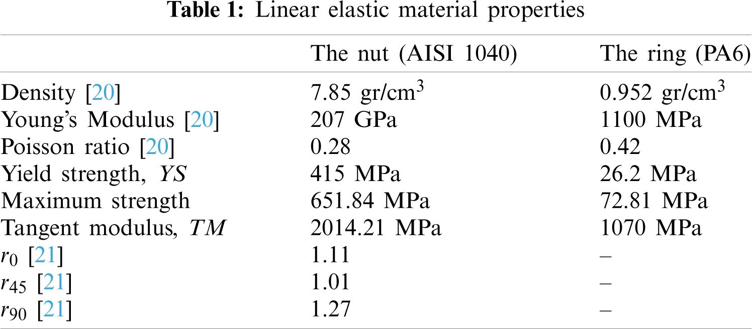

Figure 1: Specimen dimensions (units are in mm) according to (a) ASTM E7 (b) ASTM B557 M 02A

Figure 2: Monotonic uniaxial tensile curves for AISI 1040 steel and PA6
True stress-strain data was used for calculations. Kacar and Kılıç explained how to remove the elastic strain in detail [22]. The parameters of BISO model are yield strength YS and tangent modulus TM. Both were determined by using the true plastic curve [23]. Thus, the stress or strain means true stress or true strain throughout this paper.
BISO is good at modelling the material behaviour subjected to any plastic deformation in which just a monotonic loading and elastic unloading case are seen. However, it may be not enough by itself when reversal loads arise. Therefore, it is combined with CHAB. CHAB’s parameters are determined by using a hysteresis loop obtained from the low cycle fatigue testing [6].
2.2 Low Cycle Fatigue Behaviour
A low cycle fatigue test with tension-compression loads in which the strain is symmetric gives the hysteresis loops as seen in Fig. 3 for AISI 1040 steel at room temperature (full range of strains). Three strain ranges are applied as ±0.005, ±0.0075, and ±0.01 (strain ratio R = −1). Test are performed at a 25 mm/min strain rate. The strain was kept in the range ±0.01 which corresponds the strain in the folding process. To determine CHAB’s parameters, a curve-fitting algorithm based on a nonlinear regression is applied on the loops.

Figure 3: The loops for AISI 1040 steel
The maximum stress value in the tensile course is different in the compression course in one loop. Also it is seen that the stress level increases when the cycle is getting closer to the end. The Bauschinger effect and the strain hardening lead to these behaviours. In the compression course, it is very hard to keep the deformation in-plane due to buckling [24]. Therefore, Kacar et al. developed an experimental rig system by revising the grippers and specimen as in Fig. 4. So the buckling modes are sufficiently postponed [25].

Figure 4: (a) The grippers for monotonic/cyclic tests (b) The specimens
2.3 Constitutive Equations for FE Simulations
In the simulation, the material’s nonlinear mechanical behaviour is set up by using a constitutive model. The Hill48 yield criterion is used in the constitutive model [26]. The hardening rules are embedded inside the yield criterion.
A stress state can be transformed to an equivalent stress value by means of a yield criterion’s equation. Thus, it is a convenient tool to compare any stress state to the material’s yield strength to determine whether plastic deformation has started or not. A general comparison formula is given in Eq. (1).
where
where
where G, H, F, L, M, and N are the coefficients and depend on the anisotropy values, r0, r45, and r90 at 0°, 45°, and 90° with reference to the main axis. The coefficients can be calculated by formulas as in Eq. (4).
Therefore, F = 0.418, G = 0.474, H = 0.526, N = 1.341 when r0 = 1.11, r45 = 1.01, r90 = 1.27. Note that F and G are smaller than 0.5. Note that when F = 1/2, G = 1/2, H = 1/2, the Hill48 equation turns to the Von Mises equation which is another well-known yield criterion.
The isotropic term and the back stress term representing the kinematic rule are added to the comparison equation of the yield criterion as in Eq. (5). It includes both rules.
where
where YS is yield strength,
where n is the total term number to be decomposed, T is the temperature. Cm is the hardening module for mth term. It also refers to the saturation rate.
The back stress in Eq. (7) is a first order ordinary differential equation. The heat rate term can be neglected due to no temperature change during the folding process. Therefore, the equation is solved by integrating explicitly with respect to
where
Now,
When substituting Eq. (9) into Eq. (10), the yield criterion will now include BISO and CHAB rules together as seen in Eq. (11).
Similarly, it is rewritten for three back stress terms,
Actually, γ3 does not enter into the closed-form equations. A stabilized hysteresis strain-controlled loop is not enough to estimate this term. Another stress-controlled experiment is needed to determine γ3. It is used for ratcheting predictions which are out of this study’s scope. Therefore, γ3 can be given a small positive value generally [28,29]. When substituting Eq. (13) into Eq. (10), the combined model will be given by Eq. (14).
where t, c subscripts show tension, compression cases, respectively.
While the relationships between the strain and stress can be described by Hooke’s law for elastic behaviour, it is determined by a flow rule for plastic behaviour. A flow rule gives the relationship between the stress and the plastic deformation
2.4 FE Implementation of the Constitutive Model
FE simulations were performed for the folding and cyclic loading processes. Both models were used in the optimization. The final diameter and height of the locking nut were probed in addition to the stress and deformation results. The proposed optimum parameters were re-simulated in the folding process to obtain results for the diameter, height, and stress state. The simulation results were compared to experimental measurements for validation.
2.5 Optimization for Parameter Calibration
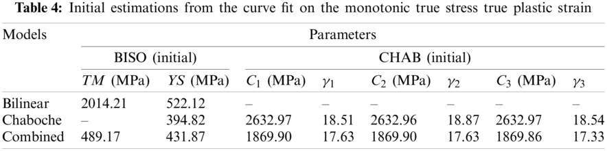
One of the techniques for calibration of just initialized material constants to obtain improvement on the general fit of the model prediction to experimental data is to use the optimization method [27,30,31]. The initially estimated material constants YS, TM, C1, γ1, C2, γ2, C3, γ3 were set as input design variables for a starting point of the optimization process. The initial values also help to inspect the lower and upper limits of variables to be studied.
An objective function was set as in Eq. (15a). By creating combinations of the design variables between lower and upper bounds in Eqs. (15b), (15c), the best-fitted parameters among them were selected by considering an objective function and constraints.
where F(x) is the objective function,
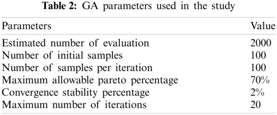
The best parameters will be the values which lead the simulation results to (almost) match the experimental results. Our goal is to minimize the difference between the measured and predicted dimensions. The goal function is set 0.5% as the convergence stability criterion. Although maximum iterations are limited to 100 as a stopping criterion for the optimization process, the most probable and physically possible points are found within 20 iterations. The convergence status during the optimization process is given in Fig. 5. 26774 evaluations are performed for the folding simulations while 11348 for the cyclic case.

Figure 5: The goal function during iterations of the optimization process
Once the simulations are completed on all design of experiment (DOE) points, now a function which will give the relations between input and output variables is fitted by means of response surfaces in the optimization module. These functions will be used to catch the optimum values along any extra points besides DOEs.
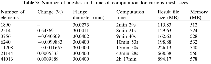
A convergence and mesh independence study was conducted in order to improve the computational efficiency as seen in Tab. 3. The mesh convergence study verifies that an accurate calculation with a minimum computation time was accomplished with a mesh having 6240 elements. Thus, the change on the results will be under 0.009%. The total computing time during the optimization for 8537 converged points takes 57 days by a computer having 3.40 GHz quad core CPU, 8 GB RAM. Totally 8 parameters,
3.1 Identification of the Model Parameters
The Chaboche’s α equation has three types of parameters as YS, Cm, γm. The number of Cm and
3.2 Optimal Parameters from Folding Simulations
The optimization process modifies the model parameters to get the more accurate folding predictions. For this purpose, a finite element model is prepared. Instead of a 3D model, an axial symmetric 2D model is used to avoid time consuming computations. A cylindrical coordinate system (x, θ, z) is located at the center point of the nut. While the axial symmetry axis is placed on the y direction, the radial direction corresponds to the x direction. The cross-section of the geometry is located at the positive side at the x axis as seen in Fig. 6. No thread is added on the FE model of the nut. Its hexagonal body is assumed cylindrical. Permanent deformation happens only at its flange.
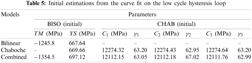

Figure 6: (a) Axial symmetric FE model of the folding process and (b) its 3D cross-section with meshes
The Coulomb friction coefficient at the tool and sample interface is assumed to be constant and taken as 0.125 for the AISI 1040 steel [37]. While the punch is modelled as a rigid body, the nut and ring are modelled as flexible bodies by assigning AISI 1040 and PA6 materials, respectively. While linear elastic material properties are applied fixed, the hardening models and their parameters in the inelastic properties are selected as design variables to the optimization. Quadrilateral planar Shell163 elements are used to create an element mesh for the nut, ring, and tool geometries. These elements have a Belytschko-TSAY element formulation with five integration points. Adaptive mesh feature has been applied to the nut to eliminate convergence errors, excessive element distortions and increase the accuracy of the simulations. Smaller elements are used on the contact edges by mesh refinement. The size of the elements gets bigger towards the outer side. The nut’s bottom edge is fixed. Similarly, the ring’s bottom surface is fixed connected to its nest. While the punch’s radial movement is constrained, a 40-stepped displacement history is applied as the load steps towards the axial direction as in Fig. 7 where a combined model with the initial parameters are used. In the beginning, the vertical gap between the punch and the nut’s flange is set as 0.6 mm. An additional 3 mm movement is provided after contact is established to ensure the strain is 0.01. The punch moves linearly towards the flange and ring. It is retracted more slowly for returning after folding.

Figure 7: Applied load steps to the punch and the height of the nut
Permanent deformation of the nut is seen after the punch goes away. When the punch starts to turn back after 20nd solution step, the height also returns from 18.2996 to 18.3918 mm because of the springback (0.5%) due to the recovery of the elastic deformation. It is seen that the springback is one of the important phenomenon on the AISI 1040 steels.
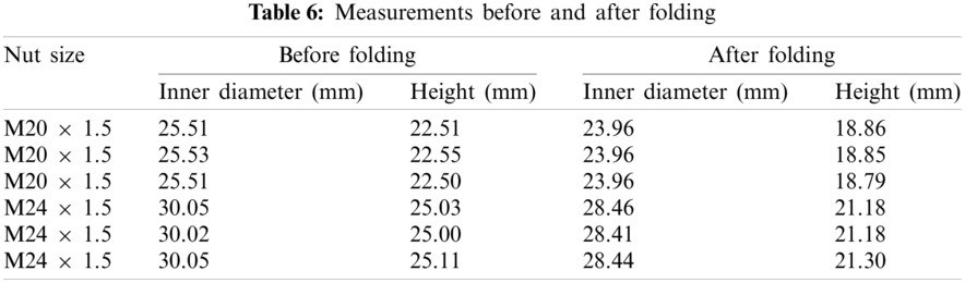
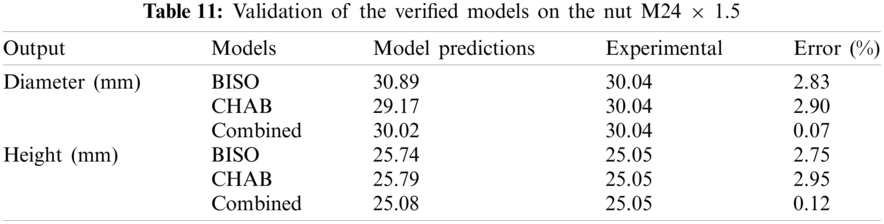
In the optimization, the folding simulations for the nut M20 × 1.5 was used. Finally, the calibrated model parameters were used in another folding simulation for the nut M24 × 1.5 for validation of the calibrated model. Validations on the real components are more reliable since they reflect the deformation conditions the best. The simulated and experimentally measured diameter and height of the nut are compared. Also the stress and strain response of the material at the scoped point are compared with the experimental hardening curve’s shape to investigate the similarity between the material response from the folding and uniaxial test. Fig. 8 shows the nut’s dimensions and scoped point. The measured values are listed in Tab. 6.

Figure 8: (a) Design variables of the nylock nut and (b) its cross-section (without the ring)
The folded height and diameter of the flange are predicted as the output. The difference between the measured and predicted dimensions will be minimized as the goal function. The constrains are applied as:
• no constraint for C, γ, and YS,
• the target for the diameter has been specified between 23.5 to 24 mm,
• the target for the nylock nut’s height has been specified between 18.5 to 19 mm after folding,
• the maximum absolute stress has been specified 1016.17 MPa for the cyclic case.
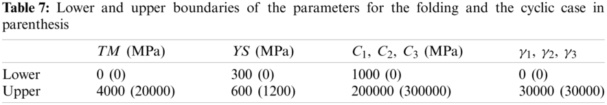
The variables’ lower and upper limits are listed in Tab. 7. 10 000 DOE points were created between these limits. The solutions were found for 8537 points. The remaining points did not converge due to inappropriate material parameter.
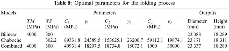
The optimization module suggests the optimum values as in Tab. 8.
3.3 Optimal Parameters from Cyclic Simulations
In addition to the folding simulations, the tension-compression test is also simulated to determine the model parameters for cyclic plasticity. A unit cylindrical model is used [38] in which no contact is required. A 25-stepped displacement history including both positive and negative values is applied as the load history. While linear elastic material properties of the AISI1040 steel are constant, the hardening model parameters are selected as design variables to the optimization. To be able to ensure that the plastic strain stays in the range of ±0.01, the reversal displacements are limited between 1.14 and −1.1 mm. The shape of the hardening loops probed from the simulation is compared with the experimental loop shape for validation. Fig. 9 shows the FE model, load history applied, and plastic strain response taken.

Figure 9: FE model and displacement steps for cyclic loading
The optimization module suggests the optimum values as in Tab. 9.
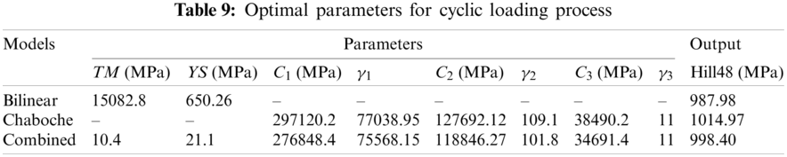
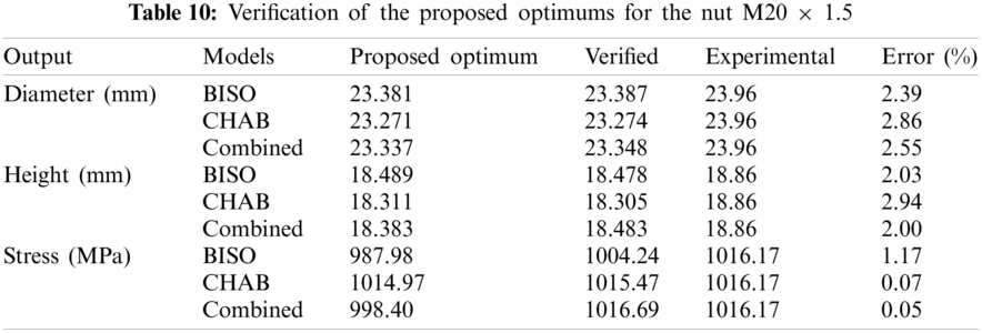
The proposed optimum values are re-simulated for verification. The percent true relative errors of the verified outputs are calculated using
For validation, a new folding simulation is performed for the nut M24 × 1.5 whose nominal diameter is
3.4 Relations between the Parameters and the Nut Size
The relationships between the parameters and the goals are obtained by means of response surface graphics created based on the Kriging method [40]. Fig. 10 shows the relations for the folding process with the combined model. Horizontal axis is normalized considering upper and lower limits of the parameters. It is seen that YS, TM, C3, and γ3 are conspicuous parameters on the diameter and height for the folding process. Increasing YS and TM leads to decrease in the deformability. C3 and γ3 have an inverse behaviour on the diameter and height.

Figure 10: The relationships between the parameters and (a) diameter (b) height
3.5 Stress and Deformation Results
When the calibrated parameters for the combined model are used in the folding simulation, the stress and deformation results are obtained as seen in Fig. 11. The graphs show the solution at the last sub step of the last step. As can be seen from the stress history, the nut undergoes plastic deformation, while the ring has only been exposed to the linear elastic deformation. The reason for the constant residual stress seen on the ring after deformation is that the contact is confirmed.

Figure 11: The stress and deformation results on the ring and nut during deformation
The Hill48 stress distribution is compared with that of the Von Mises equivalent stress. The Hill48 stress is slightly less than the Von Mises stress because F and G are smaller than 0.5. While the punch is returning after the 20th step, residual stress is seen on the nut. The nut’s body is not subjected to any plastic deformation.
Comparison of the hardening curves is the best way for validation of the parameters. The curves are compared with experimental points in reference with shape and the peak stress as seen in Figs. 12 and 13 for the AISI 1040 steel. The fitted and calibrated model predictions are also given.
The BISO model provides a linear line for hardening both before and after calibration, as expected. This linearity starts from the yield point and continues to increase with the constant slope at increasing strain values. However, the experimental behaviour of the material shows that it has a significant curvature after the yield point. For this reason, the representation ability of BISO is not sufficient. The calibration process could not improve this model. Before and after calibration, the CHAB model has a good representation for hardening behaviour. The fitted model has a bigger deviation to the prediction of the peak stress than the simulation having the calibrated models. The CHAB model starts with over-prediction with increasing strain. The combined model overcomes the over-prediction. The peak tensile stress is seen at 0.5% strain. Fitted CHAB predicts the peak stress as 959.30 MPa, while the experimental peak is 849.45 MPa leading up to 11.45% difference. Calibrated CHAB predicts 855.83 MPa leading to 0.75%. Previously a 1.6% difference was reported by Kang et al. [41]. This model is good at modelling the increasing deformation and shows a significant difference when calibrated. The curves in Figs. 12c and 13c do not have a good fit neither to experimental points nor to each other when the model parameters are used interchangeably. It is inferred that when the parameters are calibrated at a strain amplitude, simulated results deviate from experimental results at the different strain amplitudes.

Figure 12: Comparisons of hardening curves (a) fitted (b) calibrated (c) cyclic model on the folding process

Figure 13: Comparisons of cyclic hardening behaviours (a) fitted (b) calibrated (c) monotonic model on the cyclic process
When the parameters before calibration are used in the folding simulation, it is seen that there are significant differences in the loop shapes in Fig. 13a. The models are improved by modifying them in the optimization process. When optimized parameters are used, it has been found that the differences between the model and experimental loops are negligible as seen in Fig. 13b. The implemented method provides better accuracy. Therefore, these values become the calibrated material parameters.
The BISO model alone has definitely not been sufficient in modelling the cyclic behaviour as seen in Figs. 13a, 13b. Its linear nature continues after the calibration, too. CHAB or combined models show a good fit between the simulated and experimental peak tensile stress. The kinematic hardening rule is able to simulate the hysteresis loop for strain-controlled loadings as expected. Neither CHAB nor the combined model for folding has a good fit to cyclic plasticity as seen in Fig. 12c. The effects of the calibration process on the experimental strain-controlled hysteresis loops can be seen clearly when CHAB or combined models are used. Comparing the shape of the loops, it is seen that the magnitude of the error between the model and experimental data increases when getting closer to the end of the first cycle when the CHAB model is used alone. The magnitude of the error decreases when the BISO is combined with CHAB. Ramezansefat et al. [39] reported that when combined, the BISO overcomes the over-prediction problem. Usage of CHAB alone restricts the plastic flow. The combined model has the minimum over-prediction. Also the loops show close correlation to the uniaxial experiments.
Summarizing above discussions, it is concluded that one hysteresis loop from the uniaxial strain controlled test is enough to calibrate the parameters as reported by Paul et al. [42]. Although the CHAB model is expected to represent the loops well [28], it is seen that it is not sufficient when used alone, but can be used in combination [35]. In every case, calibration should be done. Researchers have used just uniaxial tests to predict the low cycle fatigue damage when calibrated by using genetic algorithm optimization methods [33,34]. It is understood that its nonlinear nature is able to reflect the nonlinearity of the material models.
This study presents parameter determination and calibration for the nut flange bending process. A plasticity model is set by using the Hill48 yield criterion, combined hardening rules, and associated flow rule for FE simulation of the flange folding process. While the BISO model’s parameters are determined from the monotonic tensile test curve, the CHAB’s parameters are determined by nonlinear regression on the experimental uniaxial hysteresis loops. The optimization process is performed to calibrate the parameters. Experiments are conducted to validate the models. Based on the analysed data, the results reveal the following;
• Although a model obtained from the tensile/compression test should not be used directly for the simulation of any multi-axial deformation process, it will be suitable as long as it is calibrated with experimental data.
• The calibrated model parameters leading to accurate folding or cyclic deformation simulation are presented for the folding process. The calibrated parameters are different for both cases. Therefore, they cannot be used interchangeably.
• While the combined hardening rule will be a good choice for cyclic deformations, all models are suitable for the folding process. By combining the BISO model with the CHAB model over-prediction is eliminated. The pure kinematic model is enough for the folding, but not enough for cyclic deformation.
• The springback shows that the AISI 1040 steel in the folding process is dependent on anisotropy. Its plastic deformability in the axial and radial directions is different. Therefore, the Hill48 criterion becomes a good choice because it can represent material anisotropy owing to its anisotropy-dependent coefficients F, G, and H.
• Residual stress on the ring does not cause any plastic deformation. Thus, the folding process can be completed without any defect on the ring.
Availability of Data and Materials: The data used in the study have already been given in the figures or tables.
Funding Statement: The author received no specific funding for this study.
Conflicts of Interest: The author declare that he has no conflicts of interest to report regarding the present study.
1. Gong, H., Liu, J., Ding, X. (2018). Effect of ramp angle on the anti-loosening ability of wedge self-locking nuts under vibration. Journal of Mechanical Design, Transactions of the ASME, 140(7), 72301. DOI 10.1115/1.4040167. [Google Scholar] [CrossRef]
2. Bhattacharya, A. S., Sen, A. K., Das, S. (2010). An investigation on the anti-loosening characteristics of threaded fasteners under vibratory conditions. Mechanism and Machine Theory, 4(8), 1215–1225. DOI 10.1016/j.mechmachtheory.2008.08.004. [Google Scholar] [CrossRef]
3. Aye, W. P. P., Htike, T. M. (2019). Inverse method for identification of edge crack using correlation model. SN Applied Sciences, 1(6), 590–596. DOI 10.1007/s42452-019-0618-x. [Google Scholar] [CrossRef]
4. Chaparro, B. M., Thuillier, S., Menezes, L. F., Manach, P. Y., Fernandes, J. V. (2008). Material parameters identification: Gradient-based, genetic and hybrid optimization algorithms. Computational Materials Science, 44(2), 339–346. DOI 10.1016/j.commatsci.2008.03.028. [Google Scholar] [CrossRef]
5. Patil, R. A., Gombi, S. L. (2020). Operational cutting force identification in end milling using inverse technique to predict the fatigue tool life. Iranian Journal of Science and Technology, Transactions of Mechanical Engineering, 42(1), 1–11. DOI 10.1007/s40997-020-00388-z. [Google Scholar] [CrossRef]
6. Agius, D., Kajtaz, M., Kourousis Kyriakos, I., Wallbrink, C., Hu, W. (2018). Optimising the multiplicative af model parameters for AA7075 cyclic plasticity and fatigue simulation. Aircraft Engineering and Aerospace Technology, 90(2), 251–260. DOI 10.1108/AEAT-05-2017-0119. [Google Scholar] [CrossRef]
7. Hassan, T., Kyriakides, S. (1992). Ratcheting in cyclic plasticity, Part I: Uniaxial behavior. International Journal of Plasticity, 8(1), 91–116. DOI 10.1016/0749-6419(92)90040-J. [Google Scholar] [CrossRef]
8. Hematiyan, M. R., Khosravifard, A., Shiah, Y. C., Tan, C. L. (2012). Identification of material parameters of two-dimensional anisotropic bodies using an inverse multi-loading boundary element technique. Computer Modeling in Engineering & Sciences, 87(1), 55–76. DOI 10.3970/cmes.2012.087.055. [Google Scholar] [CrossRef]
9. Prager, W. (1949). Recent developments in the mathematical theory of plasticity. Journal of Applied Physics, 20(3), 235–241. DOI 10.1063/1.1698348. [Google Scholar] [CrossRef]
10. Ziegler, H. (1959). A modification of prager’s hardening rule. Quarterly of Applied Mathematics, 17(1), 55–66. DOI 10.1090/qam/104405. [Google Scholar] [CrossRef]
11. Ferezqi, H. Z., Shariati, M., HadidiMoud, S. (2018). The assessment of elastic follow-up effects on cyclic accumulation of inelastic strain under displacement-control loading. Iranian Journal of Science and Technology, Transactions of Mechanical Engineering, 42(2), 127–135. DOI 10.1007/s40997-017-0089-x. [Google Scholar] [CrossRef]
12. Hatami, H., Shariati, M. (2019). Numerical and experimental investigation of SS304L cylindrical shell with cutout under uniaxial cyclic loading. Iranian Journal of Science and Technology, Transactions of Mechanical Engineering, 43(2), 139–153. DOI 10.1007/s40997-017-0120-2. [Google Scholar] [CrossRef]
13. Armstrong, P. J., Frederick, C. O. (2007). A mathematical representation of the multiaxial Bauschinger effect. Metarials at High Temperatures, 24(1), 1–26. DOI 10.3184/096034007X207589. [Google Scholar] [CrossRef]
14. Chaboche, J. L. (1989). Constitutive-equations for cyclic plasticity and cyclic viscoplasticity. International Journal of Plasticity, 5(3), 247–302. DOI 10.1016/0749-6419(89)90015-6. [Google Scholar] [CrossRef]
15. Chaboche, J. L. (1986). Time-independent constitutive theories for cyclic plasticity. International Journal of Plasticity, 2(2), 149–188. DOI 10.1016/0749-6419(86)90010-0. [Google Scholar] [CrossRef]
16. Zhao, C., Xiong, Y., Zhong, X., Shi, Z., Yang, S. (2020). A two-phase modeling strategy for analyzing the failure process of masonry arches. Engineering Structures, 212(9), 110525. DOI 10.1016/j.engstruct.2020.110525. [Google Scholar] [CrossRef]
17. Zhao, C., Zhong, X., Liu, B., Shu, X., Shen, M. (2018). A modified RBSM for simulating the failure process of RC structures. Computers and Concrete, 21(2), 219–229. DOI 10.12989/cac.2018.21.2.219. [Google Scholar] [CrossRef]
18. Zhong, X., Zhao, C., Liu, B., Shu, X., Shen, M. (2018). A 3-D RBSM for simulating the failure process of RC structures. Structural Engineering and Mechanics, 65(3), 291–302. DOI 10.12989/sem.2018.65.3.291. [Google Scholar] [CrossRef]
19. Broggiato, G. B., Campana, F., Cortese, L. (2008). The Chaboche nonlinear kinematic hardening model: Calibration methodology and validation. Meccanica, 43(2), 115–124. DOI 10.1007/s11012-008-9115-9. [Google Scholar] [CrossRef]
20. DeSalvo, G. J., Swanson, J. A. (1985). Ansys engineering analysis system user’s manual. Houston, Pa: Swanson Analysis Systems. [Google Scholar]
21. Parida, A. K., Soren, S., Jha, R. N., Sadhukhan, S. (2016). Formability of al-killed AISI, 1040 medium carbon steel for cylindrical cup formation. ISIJ International, 56(4), 610–618. DOI 10.2355/isijinternational.ISIJINT-2015-571. [Google Scholar] [CrossRef]
22. Kacar, İ., Kılıç, S. (2018). Innovative approaches in engineering, Güngör, T., Kılıç, G. B., Uyumaz, A., Görgülü, Ü.S. (Eds.pp. 175–194. Ankara, Turkey: Gece Kitaplığı. [Google Scholar]
23. Qu, F., Jiang, Z., Lu, H. (2015). Effect of mesh on springback in 3D finite element analysis of flexible microrolling. Journal of Applied Mathematics, 2015(2), 1–7. DOI 10.1155/2015/424131. [Google Scholar] [CrossRef]
24. Sharma, V. M. J., Rao, G. S., Sharma, S. C., George, K. M. (2014). Low cycle fatigue behavior of aa2219-t87 at room temperature. Materials Performance and Characterization, 3(1), 103–126. DOI 10.1520/MPC20130092. [Google Scholar] [CrossRef]
25. Kacar, İ., Toros, S. (2016). Buckling prevention conditions on cyclic test samples. 1st International Mediterranean Science and Engineering Congress, pp. 4791–4798. Adana, Turkey. [Google Scholar]
26. Hill, R. (1948). A theory of the yielding and plastic flow of anisotropic metals. Proceedings of the Royal Society of London. Series A. Mathematical and Physical Sciences, 193(1033), 281–297. DOI 10.1098/rspa.1948.0045. [Google Scholar] [CrossRef]
27. Tong, J., Zhan, Z. L., Vermeulen, B. (2004). Modelling of cyclic plasticity and viscoplasticity of a nickel-based alloy using chaboche constitutive equations. International Journal of Fatigue, 26(8), 829–837. DOI 10.1016/j.ijfatigue.2004.01.002. [Google Scholar] [CrossRef]
28. Bari, S., Hassan, T. (2000). Anatomy of coupled constitutive models for ratcheting simulation. International Journal of Plasticity, 16(3), 381–409. DOI 10.1016/S0749-6419(99)00059-5. [Google Scholar] [CrossRef]
29. Sharcnet(c) (2012). Modeling. https://www.sharcnet.ca/Software/Ansys/16.2.3/en-us/help/ans_tec/teccurv-efitchabmodel.html. [Google Scholar]
30. Gong, Y., Hyde, C., Sun, W., Hyde, T. (2009). Determination of material parameters in the chaboche unified viscoplasticty model. Applied Mechanics and Materials, 224(1), 19–29. DOI 10.1243/14644207JMDA273. [Google Scholar] [CrossRef]
31. Halama, R., Sedlak, J., Fusek, M., Poruba, Z. (2015). Uniaxial and biaxial ratcheting of St52 steel under variable amplitude loading-experiments and modeling. Procedia Engineering, 101, 185–193. DOI 10.1016/j.proeng.2015.02.024. [Google Scholar] [CrossRef]
32. Support_Ansys (1996). Video demo: Material curve fitting. https://support.ansys.com/staticassets/ANSYS/staticassets/techmedia/material_curve_fitting.html. [Google Scholar]
33. Mahmoudi, A. H., Pezeshki-Najafabadi, S. M., Badnava, H. (2011). Parameter determination of Chaboche kinematic hardening model using a multi objective genetic algorithm. Computational Materials Science, 50(3), 1114–1122. DOI 10.1016/j.commatsci.2010.11.010. [Google Scholar] [CrossRef]
34. Moslemi, N., Gol Zardian, M., Ayob, A., Redzuan, N., Rhee, S. (2019). Evaluation of sensitivity and calibration of the chaboche kinematic hardening model parameters for numerical ratcheting simulation. Applied Sciences, 9(12), 2578–2600. DOI 10.3390/app9122578. [Google Scholar] [CrossRef]
35. Nath, A., Ray, K. K., Barai, S. V. (2019). Evaluation of ratcheting behaviour in cyclically stable steels through use of a combined kinematic-isotropic hardening rule and a genetic algorithm optimization technique. International Journal of Mechanical Sciences, 152, 138–150. DOI 10.1016/j.ijmecsci.2018.12.047. [Google Scholar] [CrossRef]
36. Liu, S., Liang, G., Yang, Y. (2019). A strategy to fast determine chaboche elasto-plastic model parameters by considering ratcheting. International Journal of Pressure Vessels and Piping, 172(7), 251–260. DOI 10.1016/j.ijpvp.2019.01.017. [Google Scholar] [CrossRef]
37. Obiko, J. O., Mwema, F. M., Shangwira, H. (2020). Forging optimisation process using numerical simulation and Taguchi method. SN Applied Sciences, 2(4), 713. DOI 10.1007/s42452-020-2547-0. [Google Scholar] [CrossRef]
38. Kalnins, A., Rudolph, J., Willuweit, A. (2015). Using the nonlinear kinematic hardening material model of Chaboche for elastic-plastic ratcheting analysis. Journal of Pressure Vessel Technology-Transactions of the ASME, 137(3), 31006. DOI 10.1115/1.4028659. [Google Scholar] [CrossRef]
39. Ramezansefat, H., Shahbeyk, S. (2015). The Chaboche hardening rule: A re-evaluation of calibration procedures and a modified rule with an evolving material parameter. Mechanics Research Communications, 69, 150–158. DOI 10.1016/j.mechrescom.2015.08.003. [Google Scholar] [CrossRef]
40. Simpson, T., Mauery, T., Korte, J., Mistree, F. (1998). Comparison of response surface and kriging models for multidisciplinary design optimization. 7th AIAA/USAF/NASA/ISSMO Symposium on Multidisciplinary Analysis and Optimization, pp. 381–392. Reston, VA. [Google Scholar]
41. Kang, G., Gao, Q. (2002). Uniaxial and non-proportionally multiaxial ratcheting of U71Mn rail steel: Experiments and simulations. Mechanics of Materials, 34(12), 809–820. DOI 10.1016/S0167-6636(02)00198-9. [Google Scholar] [CrossRef]
42. Paul, S. K., Sivaprasad, S., Dhar, S., Tarafder, M., Tarafder, S. (2010). Simulation of cyclic plastic deformation response in SA333 C-Mn steel by a kinematic hardening model. Computational Materials Science, 48(3), 662–671. DOI 10.1016/j.commatsci.2010.02.037. [Google Scholar] [CrossRef]
 | This work is licensed under a Creative Commons Attribution 4.0 International License, which permits unrestricted use, distribution, and reproduction in any medium, provided the original work is properly cited. |