Computer Modeling in Engineering & Sciences

DOI: 10.32604/cmes.2021.015388

ARTICLE

Simulation of Elastic and Fatigue Properties of Epoxy/SiO2 Particle Composites through Molecular Dynamics

Gaoge Zhao, Jianzhong Chen, Yong Lv*, Xiaoyu Zhang and Li Huang

Hubei Key Laboratory of Theory and Application of Advanced Materials Mechanics, School of Science, Wuhan University of Technology, Wuhan, 430070, China
*Corresponding Author: Yong Lv. Email: lvyonghl@163.com
Received: 15 December 2020; Accepted: 08 April 2021

1  Introduction

Composite materials are used widely in the fields of aerospace, transportation, construction, machinery and industry [1–3] because of their advantages of higher strength-to-weight ratio, longer durability, and better environmental resistance compared with metal materials. Particle reinforced composite material is characterized by discontinuous particles. Its stiffness and strength are slightly lower while the material isotropy is better compared with continuous fiber reinforced material. Therefore, particle reinforced composite is still widely valued. As is known, the elastic modulus and fatigue performance are crucial indicators for particle reinforced composite.

In previous studies, the evaluation method for elastic modulus and fatigue was mainly experimental method. Some scholars have studied the effect of particle reinforcement on material elastic modulus. Su et al. [4] investigated the elastic modulus of bioinspired 3D printed two-phase composites, and found that elastic modulus generally decreases as unit cell size decreases for discontinuous phase composite. Li et al. [5] investigated the interfacial property of carbon fiber/epoxy composites and found that the interfacial property is enhanced by addition of silica nanoparticles. Also, some researchers have investigated the effects of particle reinforcement on fatigue property of composite materials. Zeltmann et al. [6] studied the fatigue property of glass fiber reinforced epoxy enhanced by nanoparticles and found that composites with small amounts of nanoparticles added into the matrix have bending fatigue strength similar to that obtained for the neat glass fiber reinforced epoxy matrix composite. As is known, the properties of materials are also closely related to the molecular structure. With the continuous improvement of computer performance, the emergence of various supercomputing platforms has greatly promoted the development of molecular dynamics simulation. Molecular dynamics is a general simulation method based on the Newtonian equations and force functions, which provides the opportunity to analyze the mechanical properties of materials on the atomic scale. Some mature theoretical systems of molecular dynamics simulation have been established. Molecular dynamics simulation has been widely used to calculate and analyze the stress-strain and failure behaviors of materials [7–9]. The development of molecular dynamics allows easy comparison of the elastic modulus of different types of materials. Adnan et al. [10] studied the influence of filler size on elastic properties of nanoparticle reinforced polymer composites using molecular dynamics simulations. Their results showed that the elastic properties of nanocomposites are significantly enhanced with the reduction of inclusion size. Similarly, the fatigue performance of materials can be simulated on the atomic scale. Some fatigue simulations [11,12] have been performed on pure polymers. In these previous studies, the creep-fatigue relationship of polymers was researched using tensile-tensile fatigue under stress-controlled conditions, and it was found that fatigue and creep cause significant changes in the van der Waals and dihedral potential energies. Besides, the fatigue behavior of amorphous polyethylene under strain-controlled conditions has been studied as well and the results show that stress relaxation is enhanced by cyclic loading.

Most of the previous works have mainly studied the fatigue property of polymers or the mechanical properties (such as elastic modulus, Poisson’s ratio, etc.) of single inclusion composite materials. There is limited research on the fatigue mechanism of composite materials and mechanical properties of randomly distributed nanoparticle materials. In this article, the mechanical properties of randomly distributed nanoparticle materials were investigated. Therefore, three models were established with different particle radii with the same mass fraction. The particle radii were 5, 8, and 12 Å, respectively. Furthermore, the fatigue performance simulation of the model with the nanoparticle radius equal of 12 Å under strain control was carried out through molecular dynamics method. Specifically, cross-linked epoxy resin was used as the composite material matrix phase and spherical SiO2 was used as the reinforcement phase.

2  Model and Simulation Details

2.1 Selection of Force Field and Construction of Molecular Model

There are some well-established force fields that can be selected to simulate the molecular system. For example, condensed-phase optimized molecular potentials for atomistic simulation studies (compass) force field, polymer consistent force field (pcff) and consistent valence force field (cvff) [13]. Yaphary et al. [14] studied the adhesion of epoxy-silica interface in salt environment using cvff and the results showed that sodium chloride solution weakens the adhesion significantly. In this work, cvff was chosen to simulate the elastic modulus and fatigue properties of nano reinforcement composite materials.

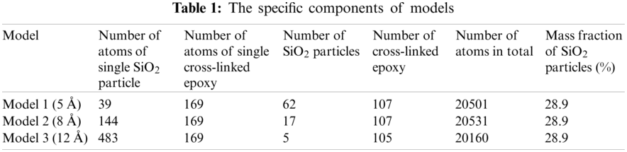
The initial model was constructed through the commercial software Material Studio (MS) 7.0, as it has a self-avoidance walking algorithm which is useful for construct a better model than others. After the initial model was constructed, the Large-scale Atomic/Molecular Massively Parallel Simulator (lammps) [15] to run molecular dynamics simulation due to the costlier computation time of MS software. 1,3-Benzenediamine was used as the curing agent and DGEBA was used as the epoxy resin in this paper, and the molecular models are shown in Figs. 1a and 1b, respectively. The reaction atoms of curing agent and epoxy resin are shown in red, named as active atom. Each curing agent can connect four epoxy resins in theory. One curing agent is employed to connect three epoxy resins as representative units of the cross-link model considering that the degree of cross-linking cannot reach 100%. The model is shown in Fig. 1c. This modeling method was applied in Yu et al. [16] and Guru et al. [17] paper and the results obtained are basically consistent with the conventional cross-link methods. Also, this method is convenient for the construction of nano reinforcement model. Figs. 1d–1f show the spherical particles with various radii. A model with low initial density was established first. However, after relaxation, the equilibrium model obtained by this model has large voids, and the structure is not reasonable. This is possibly because the initial density is not high enough. After some tests, it was found that initial density of 1.7 g/cm3 could solve the problem of voids in the equilibrium model. Then, the initial model density was set to 1.7 g/cm3 which could establish a more compact structure. The SiO2 mass fraction was set to 28.9% in this paper in order to compare the performance of different sizes of SiO2 with the same mass fraction. This mass fraction may be slightly higher than the proportion of SiO2 added in practical applications. However, it is suitable for the study of the size effect, it was worthwhile to apply. If the mass fraction of SiO2 particles is too small, it may result in only one SiO2 particle being placed when building a model with larger particles in a certain size box, which is not good for comparing the performance of random particle distribution models. Here, three models were built with 28.9% SiO2 mass fraction and nanoparticle radius of 5, 8, and 12 Å, respectively. Further increase in the particle size will result in fewer particles or even a single inclusion model, so it is not discussed herein. Figs. 2–4 present the initial model of SiO2 particles with radius of 12, 8, and 5 Å, respectively. The specific components of each model are provided in Tab. 1. The mass fraction is controlled by adjusting the number of particles and cross-linked epoxy. After the initial models were built in MS 7.0, they were converted to the lammps executable file under cvff for the molecular dynamics simulations.

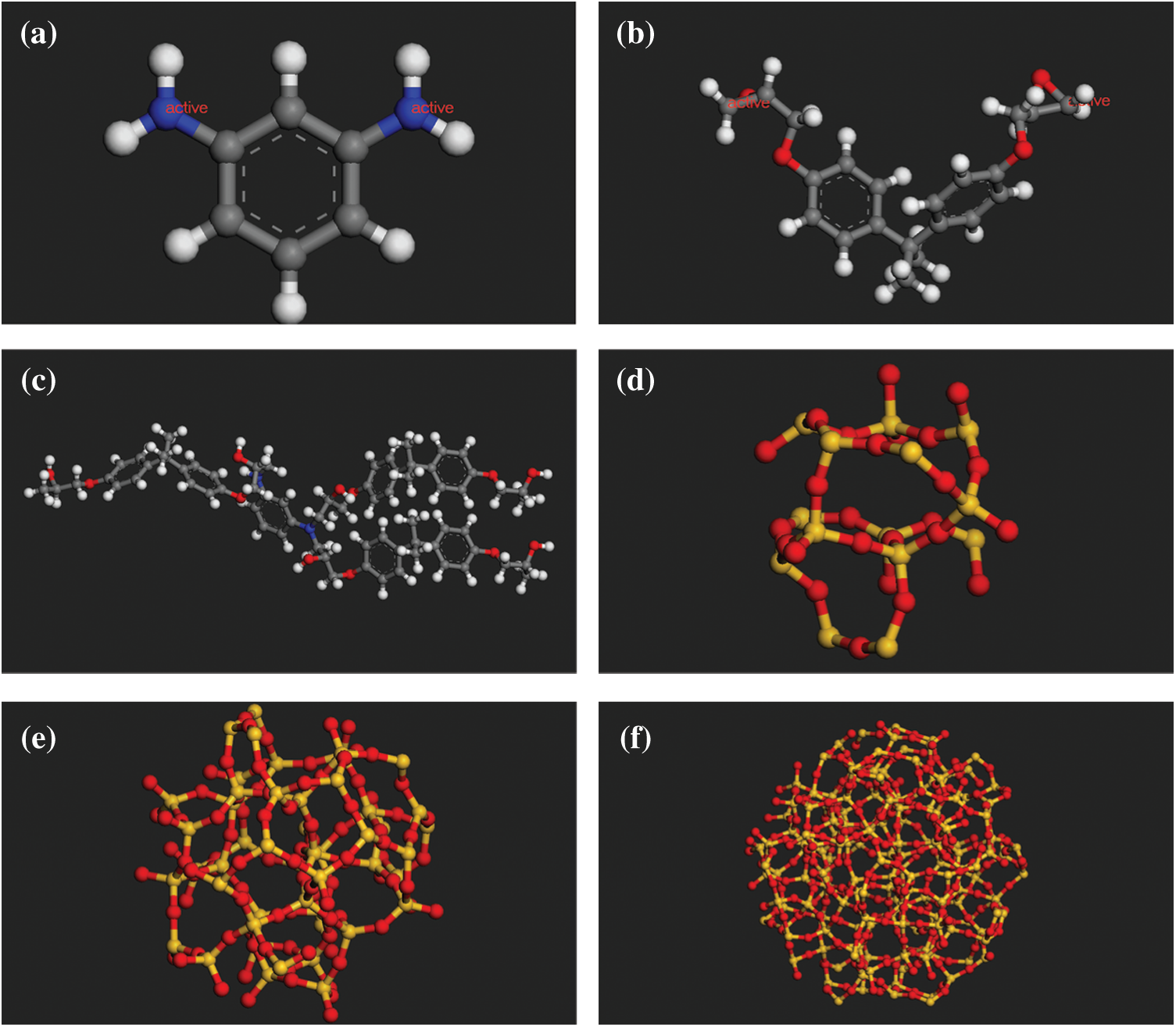
Figure 1: The molecular models of (a) 1,3-benzenediamine (b) DGEBA (c) The representative unit of cross-linked epoxy (d) Spherical SiO2 (radius of 5 Å) (e) Spherical SiO2 (radius of 8 Å) (f) Spherical SiO2 (radius of 12 Å)

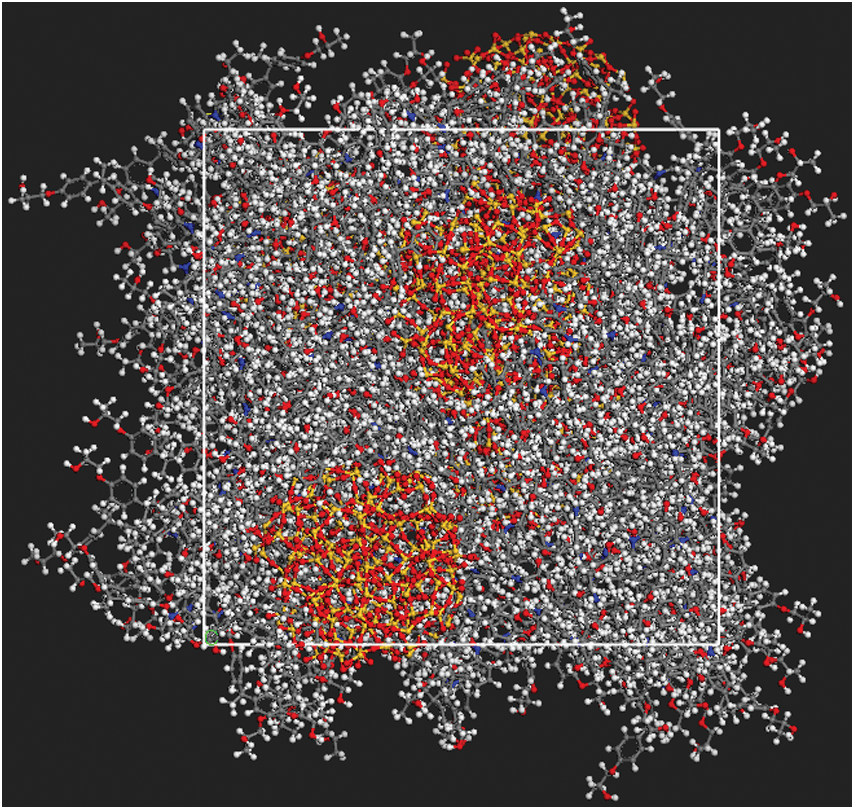
Figure 2: The initial construction of SiO2 particle with radius of 12 Å

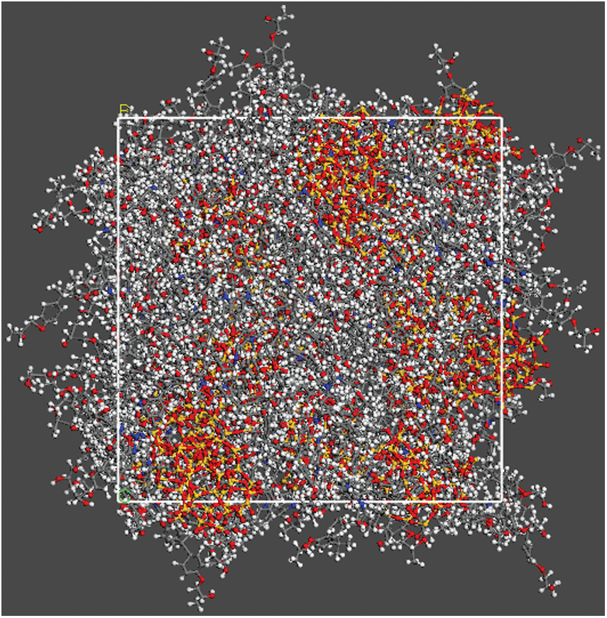
Figure 3: The initial construction of SiO2 particle with radius of 8 Å

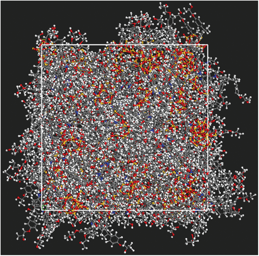
Figure 4: The initial construction of SiO2 particle with radius of 5 Å

2.2 Simulation Details

The simulation was divided into two parts: the first part was the simulation of elastic modulus of nanoparticles with different radii, including three models with particle radius of 5, 8 and 12 Å, respectively; and the second part was the simulation of the fatigue performance of the model with the particle radius equal to 12 Å. The second part was performed to compare the effects of different loading frequencies on the fatigue performance of Nano-reinforcement composite materials. Therefore, only one of these three models was selected for fatigue simulation and analysis.

2.2.1 The General Simulation Equilibrium Process of Model

A Nose–Hoover thermostat and barostat were used to control the temperature and pressure. Cut-off distance for long-range interactions was 12 Å. The entire simulation process usually includes three steps: minimizing energy, balancing the system and performance simulation. The detailed description of the three steps is given below.

(1) Energy minimizations were performed on the initial structure before running the MD simulations by applying the steepest descent algorithm which could optimize the structure to the greatest extent. Then, the conjugate gradient algorithm was employed for further optimization;

(2) The isothermal isobaric ensemble, which is abbreviated as NPT (Constant Number of particles, Pressure and Temperature) ensemble, was used to improve the structure to reach a balanced state, which is suitable for starting simulations.

During the balance process, the pressure in the three directions (x, y, z) was set to zero atmosphere. First, Gaussian distribution was used to give all particles a random speed to make the temperature of the model 100 K. Then, the system was linearly heated from 100 to 500 K through 100 picosecond (ps) simulation and simulated at 500 K for 300 ps with a time step equal to 0.5 fs. Finally, the model was cooled down to 298 K with the cooling rate equal to 1 K/ps, which was aimed to simulate temperature and relaxation for 1 ns with a time step equal to 1.0 fs at the temperature to reach the equilibrium state. After 1 ns relaxation, the densities of the models 1, 2 and 3 tend to be linear and equal 1.27, 1.28 and 1.28 g/cm3, respectively.

The final construction of equilibrium state of particle radius equal 12 Å has shown in Fig. 5 which is output from Open Visualization Tool (Ovito) [18] software, and the other models are not shown here.

(3) Next, the corresponding mechanical properties are simulated.

2.2.2 The Stress Calculation Equation

The stress tensor for atom is given by the following formula, where a and b take on values x, y, z to generate the components of the tensor in different directions:

Sab=−mvavb−Wab (1)

where the first term is a kinetic energy contribution for atom I, and the second term is the virial contribution which is shown in Eq. (2).

Wab=12∑n=1Np(r1aF1b+r2aF2b)+12∑n=1Nb(r1aF1b+r2aF2b)+13∑n=1Na(r1aF1b+r2aF2b+r3aF3b)+14∑n=1Nd(r1aF1b+r2aF2b+r3aF3b+r4aF4b)+14∑n=1Ni(r1aF1b+r2aF2b+r3aF3b+r4aF4b)+Kspace(ria,Fib) (2)

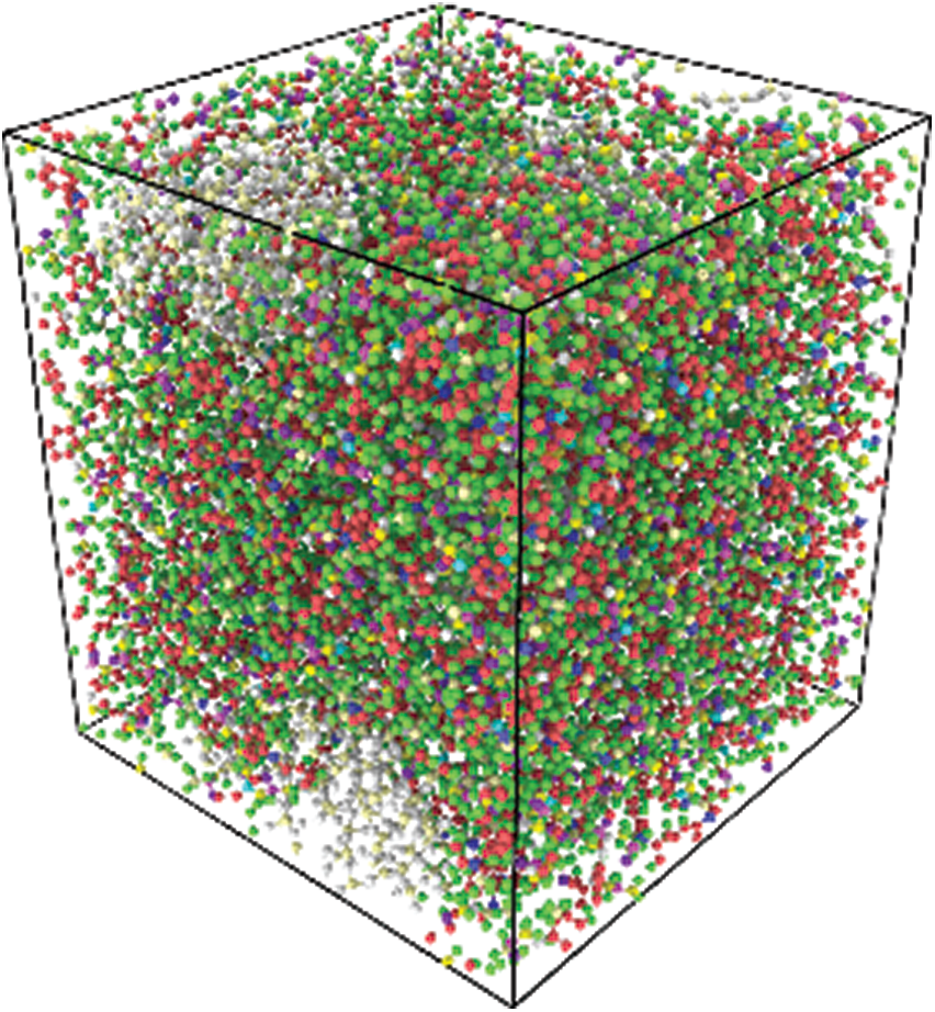
Figure 5: The construction of equilibrium state after 1 ns relaxation with SiO2 particle radius of 12 Å

The first term is a pairwise energy contribution where n loops over the Np neighbors of atom I, r1 and are the positions of the 2 atoms in the pairwise interaction, F1 and F2 are the forces on the 2 atoms resulting from the pairwise interaction. The next four terms are the contributions of similar form for the bond, angle, dihedral, and improper interactions, respectively. The last term is the K-Space contribution from long-range Coulombic interactions.

2.2.3 The Simulation Details of Elastic Modulus of Various Size Models

The calculation process of elastic modulus of three different nanoparticle size models are described below. A 5 ps equilibrium simulation was added to obtain another equilibrium conformation after the model was in equilibrium, and a further 5 ps simulation was added to obtain another equilibrium conformation in order to avoid accidental errors caused by one simulation. Finally, three slightly different equilibrium conformations were used for simulation and we take the average of the results was taken for the elastic modulus in the loading directions. The other two directions maintained a state of zero atmospheric pressure when the strain loading was applied in x direction (similarly when the loading direction is y or z). The applied strain rate was 109/s during the uniaxial tensile simulation, and take the first 3% deformation results were taken for linear fitting. The slope of fitting results represents the elastic modulus in the tensile direction.

2.2.4 The Simulation Details of Fatigue under Strain-Control

In general, fatigue can be divided into tension-compression fatigue, compression-compression fatigue and tension-tension fatigue. The tensile-tensile fatigue was applied in the simulations.

In this simulation process, the mean strain was set to 5%, and the fatigue simulation was carried out with a period equal to 1, 2, and 4 ps with a strain range of 4.5%–5.5%. The model was subjected to 5% tensile strain in x direction at a strain rate 109/s before cyclic loading.

One 400 ps simulation was performed on three different frequencies loading conditions, which have mentioned above in order to facilitate the comparison of the relationship between different loading frequencies. Therefore, that 400 cycles were simulated with a period of 1 ps, 200 cycles were simulated with a period of 2 ps, and 100 cycles were simulated with a period of 4 ps.

The loading diagram is shown in Fig. 6. Black represents period of 1 ps of the cyclic loading. Similarly, red represents period of 2 ps of the cyclic loading, and blue represents 4 ps of cyclic loading. The initial linear loading is not shown here.

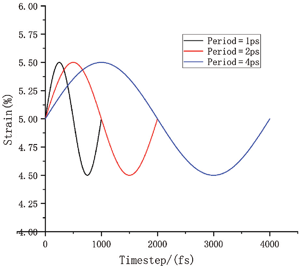
Figure 6: The diagram of one cyclic loading

3  Results and Discussion

3.1 The Result of Elastic Modulus Analysis

As shown in Tab. 2, the elastic modulus values of the individual are the average of three results. The model should be isotropic in theory, so the average of the three-direction modulus was taken as the elastic modulus of the entire model, considering that there will be deviations in the molecular models calculated in the respective directions. The results show that as the radius of the nanoparticles increases, the elastic modulus of the composite material also increases when the mass fraction is 28.9%.

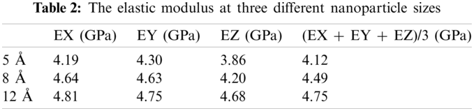
The diameter of the largest particle packing was only 2.4 nm in this simulation and the added nanoparticles could reach 100 nm and even larger in practical applications. It is reasonable to predict that the elastic modulus of the composite material gradually increase as the particle size increases within a certain range. It will be possible to use molecular simulations to calculate the size of the actually added nanoparticles on the atomic scale with the further development and application of computer computing power. The simulations can be regarded as virtual experiments to guide the design of materials for a more accurate prediction of the performance while saving time and resources.

3.2 The Result of Fatigue Analysis

In the fatigue loading, the strain loading was a standard sinusoidal curve as shown in Fig. 4. Only one model (with SiO2 radius of 12 Å) was selected for fatigue simulation and analysis as mentioned in beginning of Section 2.2. Here, the mean stress and mean strain were used to study the trend between various frequencies and the average value in one period was used as the mean stress and mean strain [9].

3.2.1 The Mean Stress vs. Number of Cycles

The relationship between the mean stress of various frequencies and the number of cycles is shown in Fig. 7. Three different loading frequencies were compared in the same period considering that time is also an important reason for the stiffness reduction of fatigue cycle. Here, we take the cycle process with a maximum period of 4 ps as a benchmark, and compare the two cycles with a period of 2 ps as one cycle. Similarly, the four cycles with a period of 1 ps are compared to one cycle. A logarithmic model, which is defined in Eq. (3), is used to fit the results.

y=a−b∗ln⁡(x) (3)

x: the number of cycles

y: the mean stress.

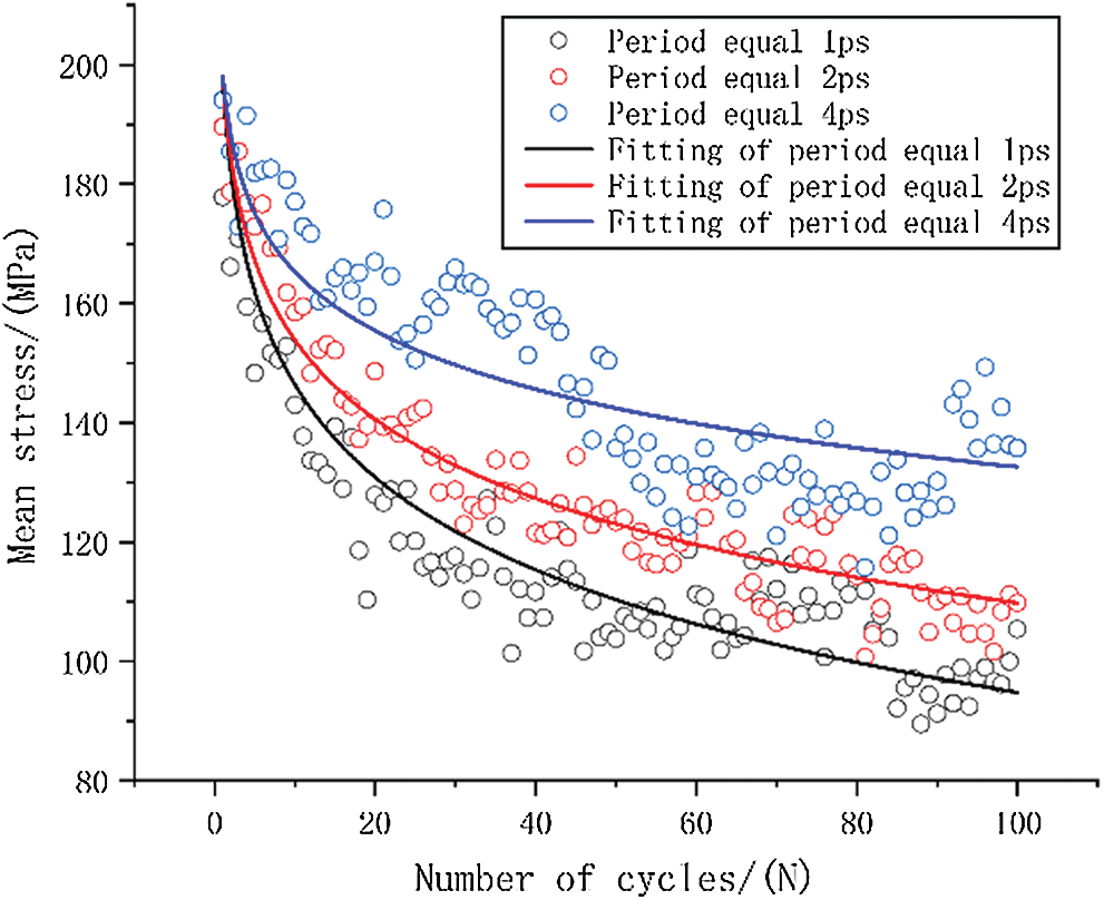
Figure 7: The origin data and curve fitting of mean stress-number of cycles

The stress level is the same stress level at the beginning of fatigue loading duo to these three loading methods use the same model. Here, the stress value is 198 MPa as the ‘a’ value of fitting equation when tensile strain is equal to 5%. The specific fitting equation is shown in Tab. 3.

It can be qualitatively inferred from the fitted curve that as the cycle period decreases, the mean stress reduces faster. This can also be quantitatively seen from the value of ‘b’ in the equation, as the smallest cycle period has the largest ‘b’ value.

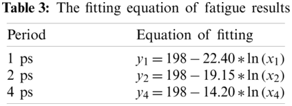
3.2.2 The Change of Energy under Fatigue State

The variation of van der Waals energy is shown in Fig. 8. The van der Waals energy with a period of 1 ps is significantly higher than the other two results, and the van der Waals energy with a period of 2 ps has a slight increase compared to the period of 4 ps. The magnitude of van der Waals energy is related to the distance between molecules. The increase of van der Waals force implies an increase in the distance between molecules in the entire simulation system. The results also show that the molecular motion is faster when the period is smaller, and it is more difficult for the molecular structure to reach a relative equilibrium state between molecules.

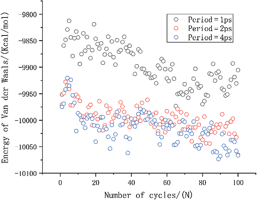
Figure 8: The change in van der Waals energy under different period loading

The mean stress reduction is greater with smaller period as expected. The smaller period has the larger value, which is the opposite of the stress reduction considering only the van der Waals energy. Hence, there should be more significant contributions from other energies. The contribution of bonded energy is mainly derived from bond tensile energy and bond angle energy. In addition, there are also contributions from dihedral angle and improper dihedral angle energy. However, these two terms have very small contributions compared with the bond tensile and bond angle energy. Therefore, only bond tensile energy and bond angle energy were analyzed here.

The result of bond tensile energy is shown in Fig. 9. It can be seen that the first several periods lead to greatly reduced mean stress when the period is 1 ps, and over all, the bond energy is also significantly smaller than other two results. This is the main reason for the faster reduction of the mean stress. It can also be seen that the bond energy of period of 2 ps is slightly smaller than that of 4 ps. The result of bond angle energy is shown in Fig. 10. It can be seen that the period of 2 ps is lower than 4 ps, and it shows a decreasing trend as the number of cycles increases. The difference in bond angle energy is the main reason why cause the mean stress of period equal to 2 ps is lower than 4 ps.

Figure 9: The change in bond energy under different period loading

3.2.3 The Free Volume Analysis under Fatigue State of Nano-Reinforcement Material

In general, the change in molecular energy is closely related to the molecular structure and distribution. The free volume change during the entire simulation process is analyzed in below.

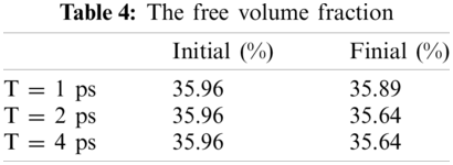
Free volume is an index for calculating the volume occupied by particles and it is based on cutting the entire box into small square grids with a size of 0.3 Å, which is enough to obtain accurate results. This grid is considered to be occupied within the van der Waals radius of the specified particle, or it is regarded as grid free and not occupied. The free volume results were processed by VMD [19] software to output higher resolution graphics after calculation by open access software Multiwfn [20]. The free volume in the case of loading with a period of 1 ps is shown here. The left image in Fig. 11 shows the distribution of particles and free volume. The blue color represents free volume and the other colors represent different types of atoms. The periodic display of x, y, and z directions is added on this basis since there is also a lot of free volume inside the model that cannot be displayed. The distribution of free volume is clearly shown in the right image of Fig. 11. The terms as same as Fig. 11 after fatigue loading at period of 1 ps is shown in Fig. 12. Although the result graphics are given with sufficient accuracy, the model is a porous structure with a large free volume and the free volume after cyclic loading will not change significantly. It is expressed in a specific numerical form as shown in the Tab. 4, the free volume when linearly loaded to 5% is 35.95%, and the free volume after 400 ps cycles is 35.89% when the period is 1ps. When the period is 2 and 4 ps, the final free volume is 35.64%.

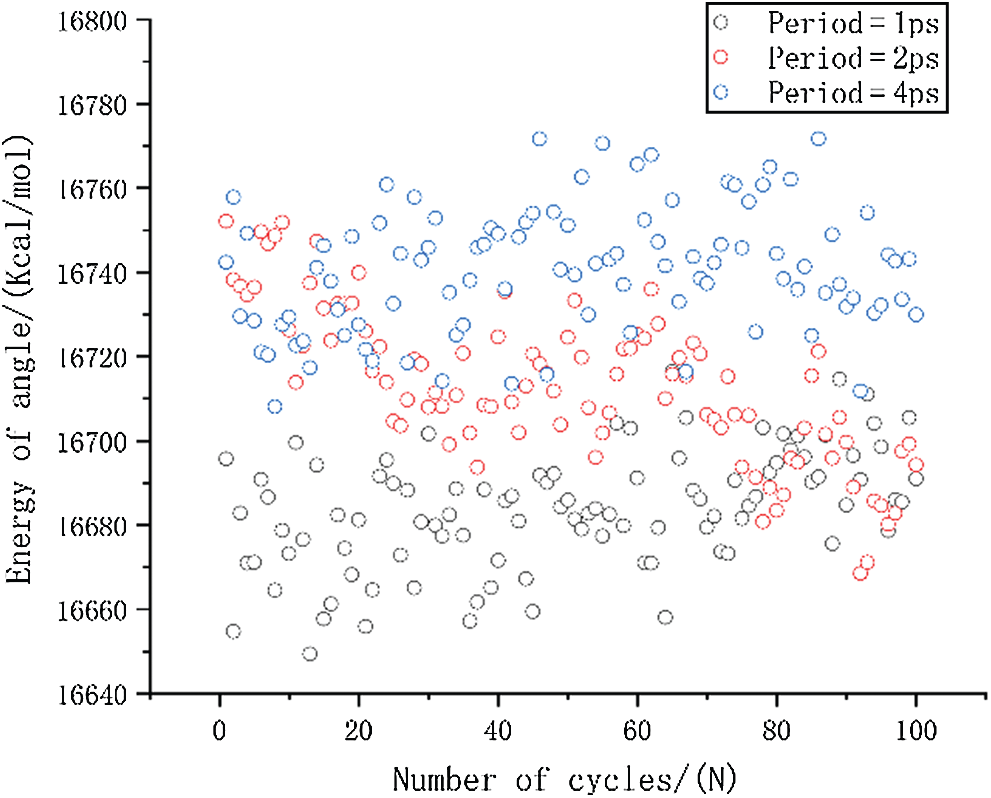
Figure 10: The change in angle energy under different period loading

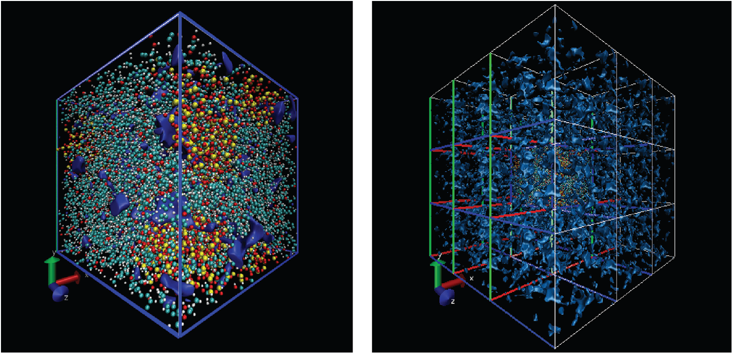
Figure 11: The free volume at initial strain of 5% (the free space is shown by blue, the left is the simulation model, the right has applied the periodic at three directions based on left)

The free volume is reduced by 0.32% when the period is 2 and 4 ps, and the free volume is only reduced by 0.07% when the period is 1 ps. The free volume reduction rate for periods of 2 and 4 ps is 4.57 times compared with periods of 1 ps. The result of this free volume change is in agreement with the result of Van der Waals energy, indicating that the smaller the period, the more difficult it is to recover the relative distance between molecules under fatigue loading. At the same time, the distance between molecules will decrease due to the relaxation effect in the loading. This result implies that the fatigue effect is higher when the period is 1ps, and the relaxation effect is not obvious. However, when the period is 2 and 4 ps, the free volume is the same and there just a slight difference in van der Waals energy between them, which indicates that the relaxation effect plays a leading role. We will continue to study this issue in depth to determine their inner connection.

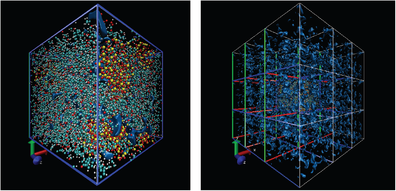
Figure 12: The free volume after fatigue loading at period of 1 ps (same as Fig. 11)

4  Conclusions

In this paper, the mechanical properties of epoxy/SiO2 particle composites with different sizes of spherical SiO2 and fatigue properties with SiO2 particle radius of 12 Å were studied using molecular dynamics, and the following conclusions were obtained:

1. As the size of the nanoparticles increases, the elastic modulus of the material increases when the mass fraction of SiO2 particle is 28.9%. This result is different from that of the single inclusion [13] model. This is because smaller SiO2 particles can agglomerate more easily, resulting in a weaker interface binding capacity with epoxy matrix, while there is no particle agglomeration phenomenon in the single inclusion model.

2. Throughout the fatigue simulation process, the van der Waals energy shows a clear downward trend, which means that the molecular gap becomes smaller as expected. At the same time, the shorter the cycle period, the higher the van der Waals energy, which means that the distance between the molecules is larger.

3. When the frequency in the fatigue loading process is higher, it is harder to achieve relative equilibrium between the molecules, and the mean stress decreases faster, which is mainly due to the lower bond energy. The main reason for the lower mean stress with a cycle period of 2 ps compared to 4 ps is the change in bond angle energy.

4. There is a relaxation effect in the fatigue process of strain control, which is similar to the creep effect of fatigue under stress control. This can also be seen from the change in free volume. The smaller the period, the less the free volume decreases. Hence, the effect of relaxation is less obvious.

Funding Statement: The project supported by the Fundamental Research Funds for the Central Universities (WUT: 2018IB001) and the Fundamental Research Funds for the Central Universities (WUT: 2019III130CG).

Conflicts of Interest: The authors declare that they have no conflicts of interest to report regarding the present study.

Appendix A. Force-Field Parameters

#data file output by msi2lmp tools

Masses

1 12.011150 # cp

2 12.011150 # c

3 12.011150 # c3

4 15.999400 # o

5 12.011150 # c2

6 12.011150 # c1

7 15.999400 # oh

8 14.006700 # n

9 1.007970 # h

10 1.007970 # ho

11 1.007970 # hn

12 28.086000 # sz

13 15.999400 # oz

Pair Coeffs # lj/cut/coul/long

1 0.1479999981 3.6170487995 # cp

2 0.1599999990 3.4745050026 # c

3 0.0389999952 3.8754094636 # c3

4 0.2280000124 2.8597848722 # o

5 0.0389999952 3.8754094636 # c2

6 0.0389999952 3.8754094636 # c1

7 0.2280000124 2.8597848722 # oh

8 0.1669999743 3.5012320066 # n

9 0.0380000011 2.4499714540 # h

10 0.0380000011 2.4499714540 # ho

11 0.0380000011 2.4499714540 # hn

12 0.0400184175 4.0534337049 # sz

13 0.2280000124 2.8597848722 # oz

Bond Coeffs # harmonic

1 480.0000 1.3400 # cp-cp

2 384.0000 1.3700 # cp-o

3 363.4164 1.0800 # cp-h

4 283.0924 1.5100 # cp-c

5 322.7158 1.5260 # c-c3

6 340.6175 1.1050 # c3-h

7 273.2000 1.4250 # o-c2

8 322.7158 1.5260 # c2-c1

9 340.6175 1.1050 # c2-h

10 322.7158 1.5260 # c3-c1

11 384.0000 1.4200 # c1-oh

12 340.6175 1.1050 # c1-h

13 377.5752 1.4600 # c2-n

14 540.6336 0.9600 # oh-ho

15 280.0000 1.4200 # cp-n

16 483.4512 1.0260 # n-hn

17 392.8000 1.6150 # sz-oz

Angle Coeffs # harmonic

1 90.0000 120.0000 # cp-cp-cp

2 60.0000 120.0000 # cp-cp-o

3 37.0000 120.0000 # cp-cp-h

4 44.2000 120.0000 # cp-cp-c

5 46.6000 110.5000 # cp-c-cp

6 46.6000 110.5000 # cp-c-c3

7 46.6000 110.5000 # c3-c-c3

8 44.4000 110.0000 # c-c3-h

9 39.5000 106.4000 # h-c3-h

10 50.0000 109.5000 # cp-o-c2

11 70.0000 109.5000 # o-c2-c1

12 57.0000 109.5000 # o-c2-h

13 44.4000 110.0000 # c1-c2-h

14 39.5000 106.4000 # h-c2-h

15 46.6000 110.5000 # c3-c1-c2

16 70.0000 109.5000 # c2-c1-oh

17 44.4000 110.0000 # c2-c1-h

18 70.0000 109.5000 # c3-c1-oh

19 44.4000 110.0000 # c3-c1-h

20 57.0000 109.5000 # oh-c1-h

21 44.4000 110.0000 # c1-c3-h

22 46.6000 110.5000 # c2-c1-c2

23 50.0000 109.5000 # c1-c2-n

24 51.5000 109.5000 # n-c2-h

25 58.5000 106.0000 # c1-oh-ho

26 102.0000 120.0000 # cp-cp-n

27 37.0000 120.0000 # cp-n-c2

28 37.5000 115.0000 # cp-n-hn

29 35.0000 122.0000 # c2-n-hn

30 37.0000 120.0000 # c2-n-c2

31 100.3000 109.4700 # oz-sz-oz

32 31.1000 149.8000 # sz-oz-sz

Dihedral Coeffs # harmonic

1 3.0000 −1 2 # cp-cp-cp-cp

2 3.0000 −1 2 # cp-cp-cp-h

3 3.0000 −1 2 # cp-cp-cp-o

4 3.0000 −1 2 # o-cp-cp-h

5 0.7500 −1 2 # cp-cp-o-c2

6 3.0000 −1 2 # h-cp-cp-h

7 3.0000 −1 2 # cp-cp-cp-c

8 3.0000 −1 2 # c-cp-cp-h

9 0.6750 1 4 # cp-cp-c-cp

10 0.0000 1 2 # cp-cp-c-c3

11 0.1581 1 3 # cp-c-c3-h

12 0.1581 1 3 # c3-c-c3-h

13 0.1300 1 3 # cp-o-c2-c1

14 0.1300 1 3 # cp-o-c2-h

15 0.1581 1 3 # o-c2-c1-c3

16 0.1581 1 3 # o-c2-c1-oh

17 0.1581 1 3 # o-c2-c1-h

18 0.1581 1 3 # h-c2-c1-c3

19 0.1581 1 3 # h-c2-c1-oh

20 0.1581 1 3 # h-c2-c1-h

21 0.1581 1 3 # h-c3-c1-c2

22 0.1581 1 3 # h-c3-c1-oh

23 0.1581 1 3 # h-c3-c1-h

24 0.1300 1 3 # c2-c1-oh-ho

25 0.1300 1 3 # c3-c1-oh-ho

26 0.1300 1 3 # h-c1-oh-ho

27 0.1581 1 3 # o-c2-c1-c2

28 0.1581 1 3 # h-c2-c1-c2

29 0.1581 1 3 # n-c2-c1-c2

30 0.1581 1 3 # n-c2-c1-oh

31 0.1581 1 3 # n-c2-c1-h

32 0.0000 1 0 # c1-c2-n-cp

33 0.0000 1 0 # c1-c2-n-hn

34 0.0000 1 0 # h-c2-n-cp

35 0.0000 1 0 # h-c2-n-hn

36 3.0000 −1 2 # cp-cp-cp-n

37 3.0000 −1 2 # n-cp-cp-h

38 2.5000 −1 2 # cp-cp-n-c2

39 2.5000 −1 2 # cp-cp-n-hn

40 0.0000 1 0 # c1-c2-n-c2

41 0.0000 1 0 # h-c2-n-c2

42 0.3000 1 3 # oz-sz-oz-sz

Improper Coeffs # cvff

1 0.0000 −1 2 # cp-cp-cp-o

2 0.3700 −1 2 # cp-cp-cp-h

3 0.3700 −1 2 # cp-cp-cp-c

4 0.3700 −1 2 # cp-cp-cp-n

5 0.0500 −1 2 # cp-n-c2-hn

6 0.3700 −1 2 # cp-n-c2-c2

7 0.0000 −1 2 # oz-sz-oz-oz

8 0.0000 −1 2 # sz-oz-sz-sz

This work is licensed under a Creative Commons Attribution 4.0 International License, which permits unrestricted use, distribution, and reproduction in any medium, provided the original work is properly cited.