| Computer Modeling in Engineering & Sciences |
DOI: 10.32604/cmes.2021.015975
ARTICLE
A Parameter-Free Approach to Determine the Lagrange Multiplier in the Level Set Method by Using the BESO
The State Key Laboratory of Digital Manufacturing Equipment and Technology, Huazhong University of Science and Technology, Wuhan, China
*Corresponding Author: Qi Xia. Email: qxia@mail.hust.edu.cn
Received: 28 January 2021; Accepted: 31 March 2021
Abstract: A parameter-free approach is proposed to determine the Lagrange multiplier for the constraint of material volume in the level set method. It is inspired by the procedure of determining the threshold of sensitivity number in the BESO method. It first computes the difference between the volume of current design and the upper bound of volume. Then, the Lagrange multiplier is regarded as the threshold of sensitivity number to remove the redundant material. Numerical examples proved that this approach is effective to constrain the volume. More importantly, there is no parameter in the proposed approach, which makes it convenient to use. In addition, the convergence is stable, and there is no big oscillation.
Keywords: Lagrange multiplier; threshold of sensitivity; BESO method; level set method; topology optimization
Among many methods for structure topology optimization [1–14], the level set method [5–10] has caught much attention. Determining the Lagrange multiplier for the constraint of material volume is an indispensable task in the level set method [15]. A straightforward approach to complete this task is to gauss a Lagrange multiplier and keep it fixed during the optimization [8], but this simple approach cannot accurately enforce the volume constraint. The second approach relies on averaging certain quantity on the boundary being optimized [9], for instance the Lagrange multiplier for the minimal compliance problem is obtained as the average of the density of strain energy on the boundary. Although this approach can accurately enforce the volume constraint, the integration on a boundary is cumbersome. The third approach is to adjust the Lagrange multiplier according to the volume of material, and it is called the augmented Lagrange multiplier method [16–18]. This approach can also accurately enforce the volume constraint. However, it is often difficult to guess a proper value of the penalty parameter in this method, hence considerable oscillations of compliance and volume usually happen as the optimization progresses. In fact, the penalty parameter significantly affects the optimization, and an improper value of the penalty parameter may even make the optimization not converge.
The approaches reviewed above are successful to determine the Lagrange multiplier. In our present study, a new approach is proposed, i.e., a parameter-free approach using the bi-directional evolutionary structural optimization (BESO) method [12,19–21]. It is inspired by the procedure for determining a threshold for material deletion and addition in the BESO. Currently, there is a trend of combining different methods of structural topology optimization [22–29] to give full play to their advantages and to complement each other, hence leading to a more powerful topology optimization method. In [22–24,28], the BESO was respectively integrated into the level set method and the phase field method to nucleate holes. In [26,27] the density method was integrated into the level set method. In [25,29] the level set method was used in the BESO to obtain smooth boundary of structures. Through the combination of different methods of structural topology optimization, several drawbacks were successfully overcome. The present study offers still another combination between the BESO method and the level set method.
2 The Level Set Based Topology Optimization
The boundary
Propagation of
where
The compliance minimization problem given by Eq. (2) is considered here
where C is the objective function;
where
Now, an important task is to determine
Although this approach can accurately enforce the volume constraint, the integration along boundary
where
When the volume of current design is larger than
Such an observation offers us the theoretical background to determine the Lagrange multiplier for the constraint of material volume in the level set method by using the BESO method.
3 Determining
BESO [12,19–21] uses sensitivity number to achieve deletion and addition of material. In the present study, the sensitivity number of the e-th element is given by [12,19]
where
3.2 Determining
Inspired by the process in the BESO method for determining the threshold
In every optimization iteration, we first compute the difference between the volume of current design (denoted as Vk) and
If
In order to delete the redundant material
In other words, the Lagrange multiplier is regarded as the threshold of sensitivity number to remove the redundant material.
Recall that the sensitivity number
As one can see in Eqs. (8) and (9), there is no parameter in the procedure to determine the Lagrange multiplier. Such a parameter-free approach is convenient to use, which is important to solve practical engineering problems. On the contrary, the widely used augmented Lagrange multiplier method is often criticized about the penalty parameter that greatly affect the results of optimization.
Note that besides using the BESO method to determine the Lagrange multiplier, we can also use it to nucleate holes during the level set based topology optimization. The details of the hole nucleation are referred to our previous papers [22–24]. Nevertheless, the method proposed in the present paper only deals with the Lagrange multiplier and has nothing to do with the hole nucleation.
In the following examples, the properties of solid material are: E = 1 and
The criteria of convergence include [19]:
and
In addition, we will terminate the optimization when k = 200.
Fig. 1 shows the design optimization problem, and
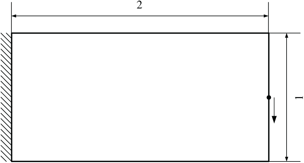
Figure 1: Design problem of Example 1
First, we do the optimization with the Lagrange multiplier being determined by using the BESO. Fig. 2 shows the initial structure and the optimized structure, and Fig. 3 shows the history of optimization. As can be seen in Fig. 3, small oscillations of compliance and volume ratio appear after the 100-th iteration. Such small oscillations have no big influence on the results of optimization. In our view, the reason of these oscillations is that the volume ratio of the structure has a small error as compared with the value required by the optimization problem.
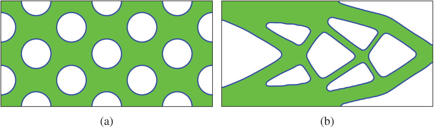
Figure 2: The initial structure and optimized structure with the Lagrange multiplier being determined by using the BESO. Compliance of (b) is 60.50, and volume is 1.00 (a) Initial structure (b) Optimized structure
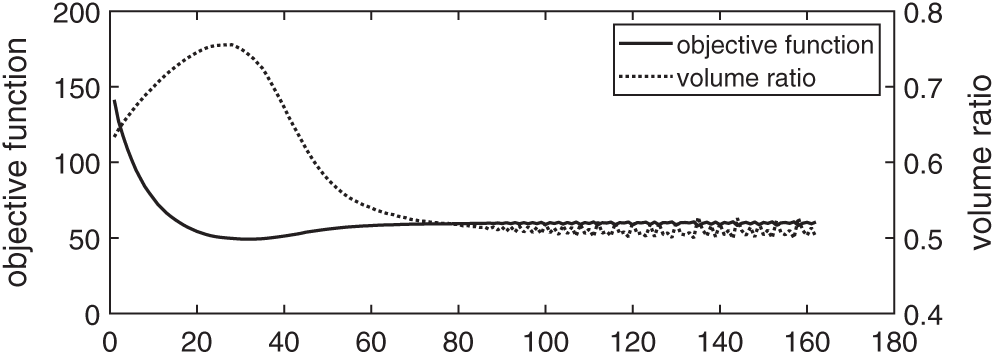
Figure 3: History of the optimization with the Lagrange multiplier being determined by using the BESO
Second, the optimization is done with the Lagrange multiplier being determined by using the augmented Lagrange multiplier method. Fig. 2a shows the initial structure. The penalty parameter in Eq. (5) is set to
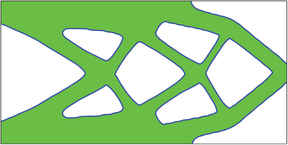
Figure 4: The optimized structure with the Lagrange multiplier being determined by using the augmented Lagrange multiplier method. Compliance of the optimized structure is 61.53, and volume is 1.00
As can be seen in Fig. 5, after
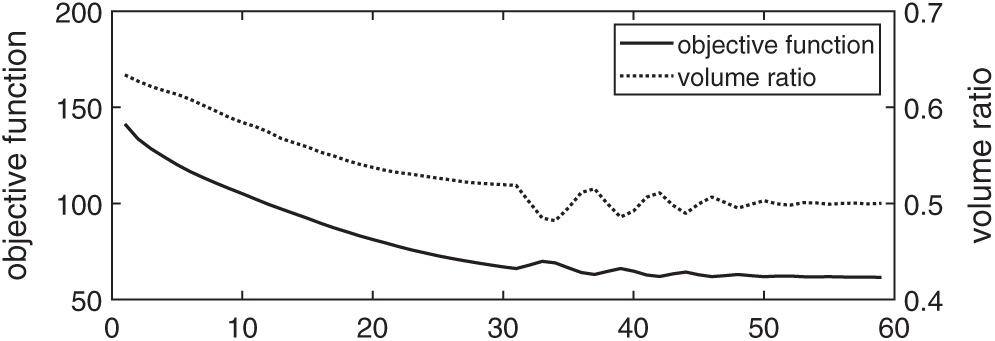
Figure 5: History of the optimization with the Lagrange multiplier being determined by using the augmented Lagrange multiplier method
From Figs. 3 and 5, we can see that there are two different kind of oscillations. First, when the optimization is near to the convergence, as can be seen in Fig. 3, the oscillations are very small, and they have no big influence on the results of optimization. Second, as shown in Fig. 5, when
The design optimization problem is shown in Fig. 6, and
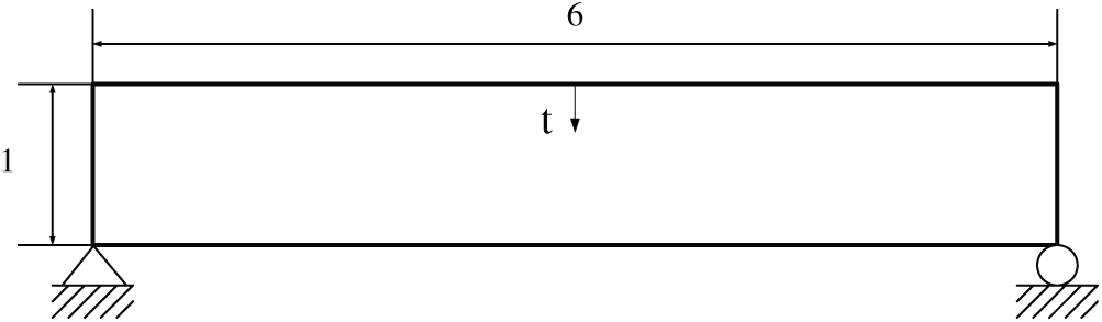
Figure 6: Design problem of Example 2
First, the optimization is done with the Lagrange multiplier being determined by using the BESO. Fig. 7 shows the initial structure and the optimized structure, and Fig. 8 shows the history of optimization. As can be seen in Fig. 8, small oscillations of compliance and volume ratio appear after the 70-th iteration. Such small oscillations have no big influence on the results of optimization.
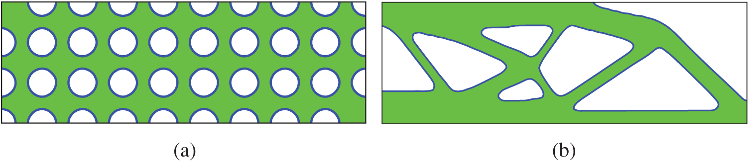
Figure 7: The initial structure and optimized structure with the Lagrange multiplier being determined by using the BESO. Compliance of the optimized structure is 183.19, and volume is 3.00 (a) Initial structure (b) Optimized structure
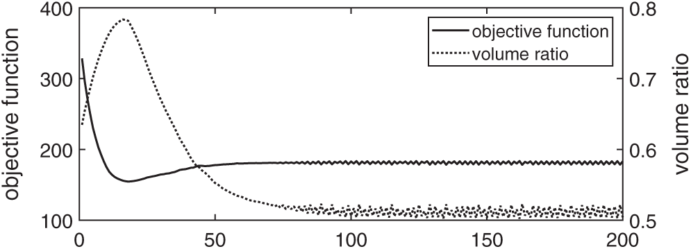
Figure 8: History of the optimization with the Lagrange multiplier being determined by using the BESO
Second, the optimization is done with the Lagrange multiplier being determined by using the augmented Lagrange multiplier method. Fig. 7a shows the initial design. The penalty parameter in Eq. (5) is set to
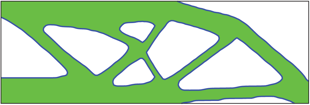
Figure 9: The optimized structure with the Lagrange multiplier being determined by using the augmented Lagrange multiplier method. Compliance of the optimized structure is 187.36, and volume is 3.00
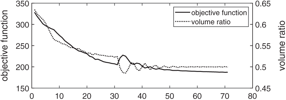
Figure 10: History of convergence of the optimization with the Lagrange multiplier being determined by using the augmented Lagrange multiplier method
Third, we put more holes into the initial design; we use a mesh with
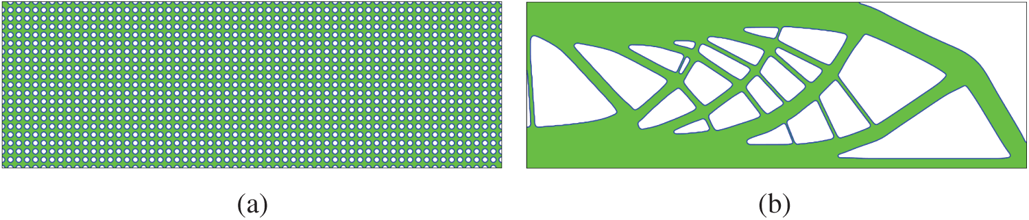
Figure 11: The initial structure and optimized structure with the Lagrange multiplier being determined by using the BESO. Compliance of the optimized structure is 183.01, and volume ratio is 0.50 (a) Initial structure (b) Optimized structure
Because the finite element mesh is finer, the threshold of sensitivity number becomes more accurate, and the Lagrange multiplier obtained by Eq. (9) is more accurate. Therefore, as can be seen in Fig. 12, there is no oscillation of compliance and volume ratio during the optimization.
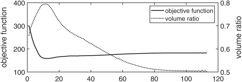
Figure 12: History of the optimization with the Lagrange multiplier being determined by using the BESO
The design optimization problem is shown in Fig. 13, and
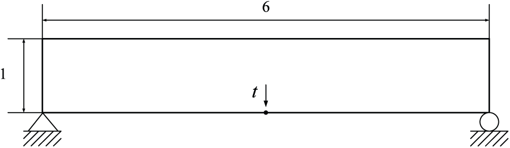
Figure 13: Design problem of Example 3
First, we do the optimization with the Lagrange multiplier being determined by using the BESO. Fig. 14 shows the initial structure and the optimized structure, and Fig. 15 shows the history of optimization. As can be seen in Fig. 15, small oscillations of compliance and volume ratio appear after the 120-th iteration. Fig. 16 shows serval intermediate designs, and one can see that the optimization first defines the solid outer skin of the structure, meanwhile many small holes are remained in the inner region. At this time, the porous inner region may be regarded as a region filled with microstructures. Then, as the optimization progresses, some thin beams appear in the optimized structure.
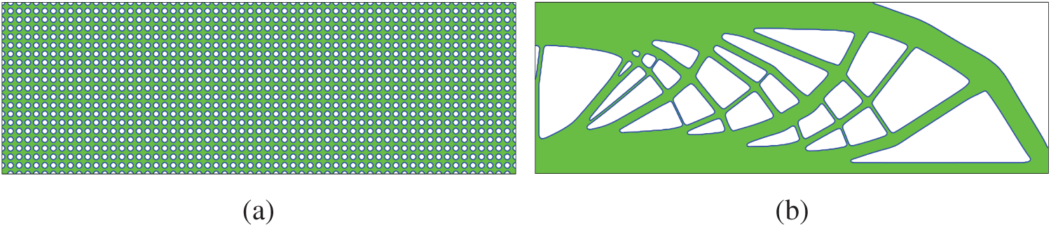
Figure 14: The initial structure and optimized structure with the Lagrange multiplier being determined by using the BESO. Compliance of the optimized structure is 182.93, and volume is 3.00 (a) Initial structure (b) Optimized structure
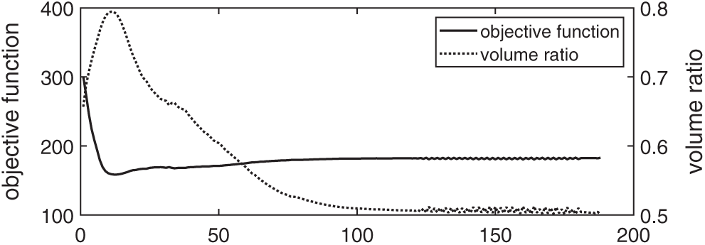
Figure 15: History of the optimization with the Lagrange multiplier being determined by using the BESO
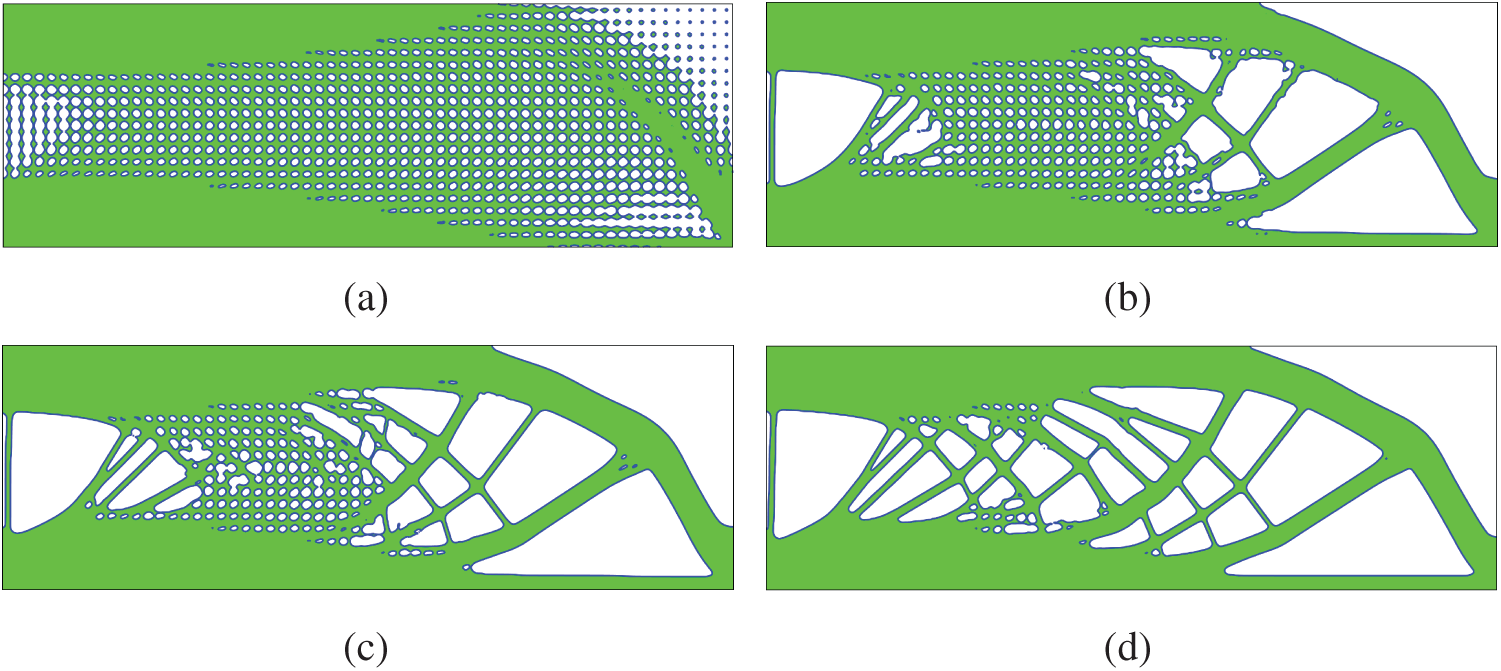
Figure 16: Intermediate designs of the third example with the Lagrange multiplier determined by using BESO (a) Step 20 (b) Step 5 (c) Step 60 (d) Step 80
Second, besides using the BESO to determine the Lagrange multiplier, we also use the BESO to nucleate hole. The details of the hole nucleation are referred to our previous papers [22–24]. Fig. 17 shows the initial structure and the optimized structure, and Fig. 18 shows the history of optimization. One can see that the converge is smooth. Several intermediate designs are shown in Fig. 19.

Figure 17: The initial structure and optimized structure with the Lagrange multiplier and hole nucleation achieved by using BESO. Compliance of the optimized structure is 183.79, and volume ratio is 0.50 (a) Initial structure (b) Optimized structure
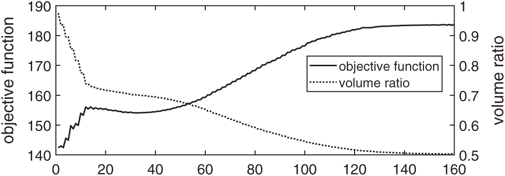
Figure 18: History of convergence of the optimization with the Lagrange multiplier and hole nucleation achieved by using BESO
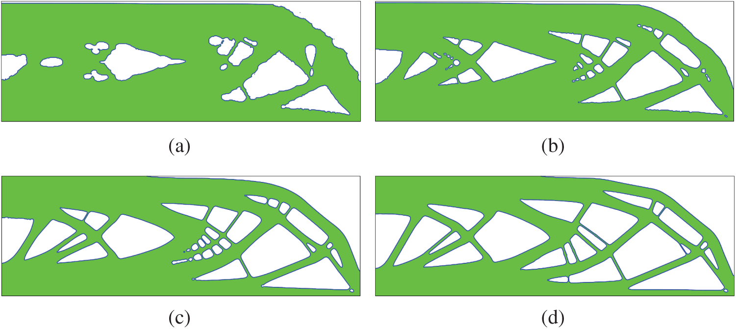
Figure 19: Intermediate designs of the third example with the Lagrange multiplier and hole nucleation achieved by using BESO (a) Step 10 (b) Step 20 (c) Step 70 (d) Step 110
Determining the Lagrange multiplier for the constraint of material volume is an indispensable task in the level set method. Although the approaches that can be found in the literature are successful, they also suffer from some drawbacks. In this paper, a new approach is proposed to determine the Lagrange multiplier. First, it computes the difference between the volume of current design and the upper bound of volume. Then, the Lagrange multiplier is regarded as the threshold of sensitivity number to remove the redundant material. Several numerical examples demonstrated that this approach is effective. More importantly, there is no parameter in the proposed approach, which makes it convenient to use. In addition, the convergence is stable, and there is no big oscillation. In the future, the proposed approach will be further extended to deal with other optimization problems or other constraints, for instance, the microstructure optimization [31] or the fatigue damage [32].
Funding Statement: This research work is supported by the National Natural Science Foundation of China (Grant No. 51975227).
Conflicts of Interest: The authors declare that they have no conflicts of interest to report regarding the present study.
1. Bendsøe, M. P., Kikuchi, N. (1988). Generating optimal topologies in structural design using a homogenization method. Computer Methods in Applied Mechanics and Engineering, 71(2), 197–224. DOI 10.1016/0045-7825(88)90086-2. [Google Scholar] [CrossRef]
2. Bendsøe, M. P. (1989). Optimal shape design as a material distribution problem. Structural Optimization, 1(4), 193–202. DOI 10.1007/BF01650949. [Google Scholar] [CrossRef]
3. Rozvany, G. I. N., Zhou, M., Birker, T. (1992). Generalized shape optimization without homogenization. Structural Optimization, 4(3), 250–254. DOI 10.1007/BF01742754. [Google Scholar] [CrossRef]
4. Sigmund, O. (2001). A 99 line topology optimization code written in MATLAB. Structural and Multidisciplinary Optimization, 21(2), 120–127. DOI 10.1007/s001580050176. [Google Scholar] [CrossRef]
5. Sethian, J. A., Wiegmann, A. (2000). Structural boundary design via level set and immersed interface methods. Journal of Computational Physics, 163(2), 489–528. DOI 10.1006/jcph.2000.6581. [Google Scholar] [CrossRef]
6. Osher, S., Santosa, F. (2001). Level-set methods for optimization problems involving geometry and constraints: Frequencies of a two-density inhomogeneous drum. Journal of Computational Physics, 171(1), 272–288. DOI 10.1006/jcph.2001.6789. [Google Scholar] [CrossRef]
7. Allaire, G., Jouve, F., Toader, A. M. (2002). A level-set method for shape optimization. Comptes Rendus Mathematique, 334(12), 1–6. DOI 10.1016/S1631-073X(02)02412-3. [Google Scholar] [CrossRef]
8. Allaire, G., Jouve, F., Toader, A. M. (2004). Structural optimization using sensitivity analysis and a level-set method. Journal of Computational Physics, 194(1), 363–393. DOI 10.1016/j.jcp.2003.09.032. [Google Scholar] [CrossRef]
9. Wang, M. Y., Wang, X. M., Guo, D. M. (2003). A level set method for structural topology optimization. Computer Methods in Applied Mechanics and Engineering, 192(7), 227–246. DOI 10.1016/S0045-7825(02)00559-5. [Google Scholar] [CrossRef]
10. Wang, M. Y., Wang, X. M. (2004). PDE-driven level sets, shape sensitivity and curvature flow for structural topology optimization. Computer Modeling in Engineering & Sciences, 6(4), 373–395. DOI 10.3970/cmes.2004.006.373. [Google Scholar] [CrossRef]
11. Xie, Y. M., Steven, G. P. (1993). A simple evolutionary procedure for structural optimization. Computers & Structures, 49(5), 885–896. DOI 10.1016/0045-7949(93)90035-C. [Google Scholar] [CrossRef]
12. Huang, X. D., Xie, Y. M. (2007). Convergent and mesh-independent solutions for the bidirectional evolutionary structural optimization method. Finite Elements in Analysis and Design, 43(14), 1039–1049. DOI 10.1016/j.finel.2007.06.006. [Google Scholar] [CrossRef]
13. Guo, X., Zhang, W. S., Zhong, W. L. (2014). Doing topology optimization explicitly and geometrically—A new moving morphable components based framework. Journal of Applied Mechanics, 81(8), 81009. DOI 10.1115/1.4027609. [Google Scholar] [CrossRef]
14. Zhang, W. S., Yuan, J., Zhang, J., Guo, X. (2016). A new topology optimization approach based on moving morphable components (MMC) and the ersatz material model. Structural and Multidisciplinary Optimization, 53(6), 1243–1260. DOI 10.1007/s00158-015-1372-3. [Google Scholar] [CrossRef]
15. Van Dijk, N., Maute, K., Langelaar, M., Van Keulen, F. (2013). Level-set methods for structural topology optimization: A review. Structural and Multidisciplinary Optimization, 48(3), 437–472. DOI 10.1007/s00158-013-0912-y. [Google Scholar] [CrossRef]
16. Belytschko, T., Xiao, S. P., Parimi, C. (2003). Topology optimization with implicit functions and regularization. International Journal for Numerical Methods in Engineering, 57(8), 1177–1196. DOI 10.1002/nme.824. [Google Scholar] [CrossRef]
17. Wei, P., Wang, M. Y. (2006). The augmented lagrangian method in structural shape and topology optimization with RBF based level set method. The Forth China-Japan-Korea Joint Symposium on Optimization of Structural and Mechanical Systems, pp. 1–6, Kunming, China. [Google Scholar]
18. Xia, Q., Wang, M. Y. (2008). Topology optimization of thermoelastic structures using level set method. Computational Mechanics, 42(6), 837–857. DOI 10.1007/s00466-008-0287-x. [Google Scholar] [CrossRef]
19. Huang, X., Xie, M. (2010). Evolutionary topology optimization of continuum structures: Methods and applications. UK: John Wiley & Sons. [Google Scholar]
20. Huang, X. D., Xie, Y. M. (2008). A new look at ESO and BESO optimization methods. Structural and Multidisciplinary Optimization, 35(1), 89–92. DOI 10.1007/s00158-007-0140-4. [Google Scholar] [CrossRef]
21. Huang, X. D., Xie, Y. M. (2009). Bi-directional evolutionary topology optimization of continuum structures with one or multiple materials. Computational Mechanics, 43(3), 393–401. DOI 10.1007/s00466-008-0312-0. [Google Scholar] [CrossRef]
22. Xia, Q., Shi, T. L., Xia, L. (2019). Stable hole nucleation in level set based topology optimization by using the material removal scheme of BESO. Computer Methods in Applied Mechanics and Engineering, 343, 438–452. DOI 10.1016/j.cma.2018.09.002. [Google Scholar] [CrossRef]
23. Xia, Q., Shi, T. L. (2019). Generalized hole nucleation through BESO for the level set based topology optimization of multi-material structures. Computer Methods in Applied Mechanics and Engineering, 355, 216–233. DOI 10.1016/j.cma.2019.06.028. [Google Scholar] [CrossRef]
24. Xia, Q., Shi, T. L., Xia, L. (2018). Topology optimization for heat conduction by combining level set method and BESO method. International Journal of Heat and Mass Transfer, 127, 200–209. DOI 10.1016/j.ijheatmasstransfer.2018.08.036. [Google Scholar] [CrossRef]
25. Da, D. C., Xia, L., Li, G. Y., Huang, X. D. (2018). Evolutionary topology optimization of continuum structures with smooth boundary representation. Structural and Multidisciplinary Optimization, 57(6), 2143–2159. DOI 10.1007/s00158-017-1846-6. [Google Scholar] [CrossRef]
26. Wei, P., Wang, W. W., Yang, Y., Wang, M. Y. (2020). Level set band method: A combination of density-based and level set methods for the topology optimization of continuums. Frontiers of Mechanical Engineering, 15(3), 390–405. DOI 10.1007/s11465-020-0588-0. [Google Scholar] [CrossRef]
27. Barrera, J. L., Geiss, M. J., Maute, K. (2020). Hole seeding in level set topology optimization via density fields. Structural and Multidisciplinary Optimization, 61(1), 1319–1343. DOI 10.1007/s00158-019-02480-8. [Google Scholar] [CrossRef]
28. Gao, J. W., Song, B. W., Mao, Z. Y. (2020). Combination of the phase field method and BESO method for topology optimization. Structural and Multidisciplinary Optimization, 61(1), 225–237. DOI 10.1007/s00158-019-02355-y. [Google Scholar] [CrossRef]
29. Huang, X. D. (2021). On smooth or 0/1 designs of the fixed-mesh element-based topology optimization. Advances in Engineering Software, 151, 102942. DOI 10.1016/j.advengsoft.2020.102942. [Google Scholar] [CrossRef]
30. Xia, Q., Wang, M. Y., Shi, T. L. (2013). A move limit strategy for level set based structural optimization. Engineering Optimization, 45(9), 1061–1072. DOI 10.1080/0305215X.2012.720681. [Google Scholar] [CrossRef]
31. Wang, Y. J., Liao, Z. Y., Shi, S. Y., Wang, Z. P., Poh, L. H. (2020). Data-driven structural design optimization for petal-shaped auxetics using isogeometric analysis. Computer Modeling in Engineering & Sciences, 122(2), 433–458. DOI 10.32604/cmes.2020.08680. [Google Scholar] [CrossRef]
32. Chen, Z., Long, K., Wen, P., Nouman, S. (2020). Fatigue-resistance topology optimization of continuum structure by penalizing the cumulative fatigue damage. Advances in Engineering Software, 150, 102924. DOI 10.1016/j.advengsoft.2020.102924. [Google Scholar] [CrossRef]
 | This work is licensed under a Creative Commons Attribution 4.0 International License, which permits unrestricted use, distribution, and reproduction in any medium, provided the original work is properly cited. |