Computer Modeling in Engineering & Sciences

DOI: 10.32604/cmes.2021.016494

ARTICLE

The Effect of Key Design Parameters on the Global Performance of Submerged Floating Tunnel under Target Wave and Earthquake Excitations

Chungkuk Jin* and MooHyun Kim

Department of Ocean Engineering, Texas A&M University, College Station, TX 77843, USA
*Corresponding Author: Chungkuk Jin. Email: jinch999@tamu.edu
Received: 10 March 2021; Accepted: 08 May 2021

1  Introduction

The Submerged Floating Tunnel (SFT) has recently attracted significant attention as an alternative to conventional bridges and immersed tunnels for long-distance and deepwater crossing [1]. It is a simple structure consisting of a tunnel at a target submergence depth and mooring lines. It has potential advantages: the construction cost per unit length is relatively irreverent to a tunnel length, the ship traffic problem can be solved by keeping submergence depth more than 30 m, and an optimal design can be safe against both waves and earthquakes.

Active studies related to SFTs have been conducted with respect to a variety of environmental conditions for achieving the first real construction. Developing a robust and time-efficient simulation model is recognized as one of the essential tasks, especially for SFT research due to its potentially high deformability. There exist few experimental studies associated with the dynamics of SFT in waves [2–4] and currents [5]. They built a model-scale rigid tunnel module connected with mooring lines to investigate the effects of various system parameters, including Buoyancy-Weight Ratio (BWR), submergence depth, and inclination angles of mooring lines, on the global performance. However, the longitudinal structural flexibility is an important part of this kind of elastic object, but it is challenging to implement the long structure as a correctly scaled physical model. Then, the actual hydro-elastic behavior of the long structure needs to be numerically simulated by using reliable and validated computer programs. Based on this background, high-fidelity simulations play a crucial role in optimizing the design. Many researchers considered the structure's elasticity under wave [6–8] and earthquake [9,10] excitations. Most of them adopted the Morison-force model to estimate the hydrodynamic force on SFTs because it provided reasonable results on such slender structures. Besides, the Morison formula is a time-efficient force-estimation method compared with other more complicated hydro-elasticity methods, such as the BEM-FEM direct coupling [11,12], modal superposition with BEM including elastic modes [13], and discrete-module-beam methods with multi-body BEM [14,15]. In particular, the Morison model can be utilized as an effective tool for design-parameter optimization.

Until now, most studies concentrated on theoretical investigations and parametric studies. For example, regarding wave excitations, Lu et al. [16] investigated the snap loading phenomenon associated with BWR and mooring inclination angle. High wave heights and low BWRs are prone to snap loading resulting in substantially increased mooring tension. Sharma et al. [17] showed the role of a bottom-mounted submerged porous breakwater for SFT dynamics. Jin et al. [18] proposed coupled dynamics simulations based on the potential theory for a rigid tunnel segment. Yarramsetty et al. [19] showed the importance of considering nonlinear cables by comparing linear and nonlinear cable dynamics. Concerning earthquake excitations, Di Pilato et al. [20] conducted coupled dynamics simulations under earthquake excitations, demonstrating the importance of earthquake excitations in SFT dynamic responses. Xie et al. [21] and Lee et al. [22] investigated earthquake-induced waves and their influences on tunnel dynamics. Martinelli et al. [23] presented a detailed procedure for producing artificial ground motions and conducted the structural analysis under the generated seismic motions. Jin et al. [10] performed SFT-train coupled simulations under earthquake excitations. These examples provide detailed information to understand the basics of the SFT's dynamic characteristics.

There exist technical difficulties in the construction of the structure. One of the critical problems for the large diameter tunnel is considerable dynamic tension, which is usually due to snap loading. Higher BWR is recommended to resolve the snap loading, as also in [16], which in turn increases the static tension. Short mooring intervals are needed to distribute the high mooring tension among neighboring mooring lines; however, it leads to more mooring/anchor installation and the resulting high installation cost. Various factors can contribute to these high mooring tensions, and thus a practical guideline for designing large SFT can be different depending on the environmental conditions and submergence depths at a target location.

In this study, a practical strategy for the SFT design is presented. Coupled time-domain hydro-elastic simulations for large SFT are conducted in wave and earthquake conditions. The tunnel and mooring lines are separately modeled with a finite-element line model based on the lumped mass method. Each component is divided into several finite elements to account for structural deformability. Their connection is completed by the dummy-connection-method [24] and constraint condition specially proposed for SFT research by authors. The Morison equation estimates both wave- and earthquake-induced hydrodynamic forces. Different locations have different wave and earthquake conditions. For instance, the 100-year storm condition in the South-Korean Sea is much harsher than that in Norwegian fjords. In this regard, we consider different magnitudes of wave and earthquake excitations. Besides, systematic parametric studies are performed under different BWRs, submergence depths, tunnel lengths, and mooring intervals to find appropriate design strategies to reduce maximum mooring tensions.

2  Time-Domain Formulation

A coupled time-domain model is established by OrcaFlex, a widely-used commercial program in the oil and gas industry [25]. 2D drawings of the proposed SFT used in this study and an example numerical model by OrcaFlex are presented in Fig. 1. Since the structure is highly deformable, the entire SFT is modeled with the line model that can represent elastic behavior. The line model is made up of N nodes (lumped masses) and N−1 connecting elements (linear springs) between nodes, as illustrated in Fig. 2. Physical properties, such as mass, drag, and buoyancy, are lumped at the nodes, while structural deformability is represented by massless springs. Formulations for structural forces in the line model are presented in Appendix A. Equation of motion for SFT can be expressed as:

Mx¨+Cx˙+Kx=FM+w~+FC(1)

where M is the mass matrix, C and K are the structural damping and stiffness matrices, x is the displacement vector, FM is the total hydrodynamic force vector, w~ is the wet weight vector, FC is the constraint force vector originated by the coupling effect between the tunnel and mooring lines at the corresponding connection locations. The upper dot in the formulations means the time derivative of a variable.

Cx˙ stands for structural damping, which is a crucial component to damp the resonant responses effectively. The structural damping considers the internal friction and composite interaction between materials during the deformation. In this study, the mass and stiffness proportional Rayleigh damping model is selected owing to its practicality and reliability, which can be expressed as:

C=αMT+βK(2)

where α and β are the mass and stiffness proportional damping coefficients, and MT is the total mass matrix including the added mass. When the damping ratio ζ is known and identical at the two structural modes i and j, α and β can be calculated as:

α=ζ2ωn,iωn,jωn,i+ωn,j(3)

β=ζ2ωn,i+ωn,j(4)

where ωn is natural frequency. Based on the above formulations, it can be noticed that α and β play a prominent role in damping low- and high-frequency excitations, respectively. 5% ζ is widely selected for concrete structures, which is also adopted in this system at the lowest lateral and vertical modes to estimate structural damping. The natural frequencies are obtained by modal analysis of the coupled system after static simulation.

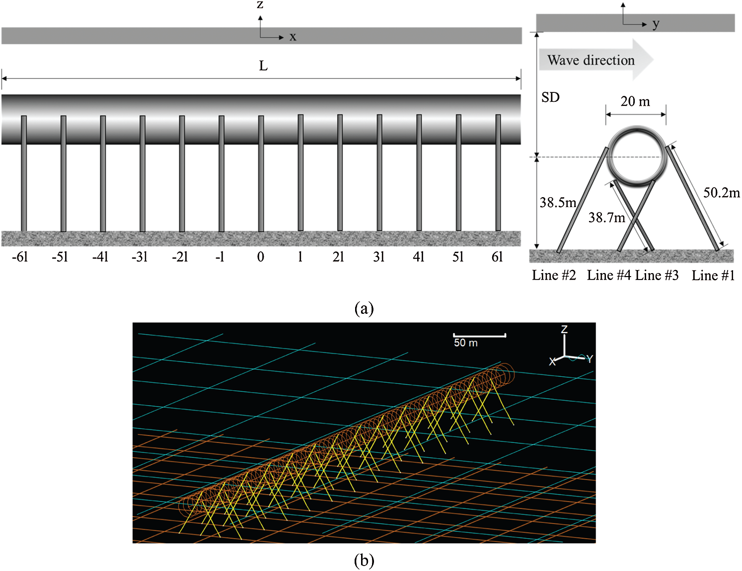
Figure 1: SFT configuration (L = total length, l = mooring interval, SD = submergence depth) (a) and representative numerical model (L = 700 m) by OrcaFlex (b)

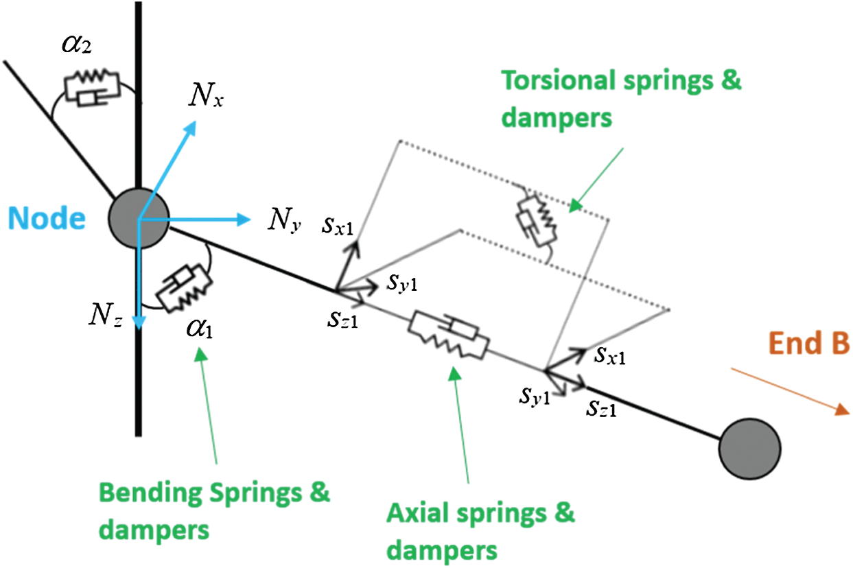
Figure 2: Line model [25]

Kx describes the structural deformability with axial, bending, and torsional springs. As described in Fig. 2, tension and torsional behaviors are represented by axial and torsional springs located at the center of two adjacent nodes, while bending springs at either side of the node estimate bending behaviors.

FM is estimated by the Morison equation for a moving body, calculated at the instantaneous node positions as:

FM=−CAρΔx¨n+CMρΔV˙n+12CDρA|Vn−x˙n|(Vn−x˙n)(5)

where CA, CM, and CD are, respectively, the added mass, inertia, and drag coefficients, ρ is the density of the surrounding fluid, Δ is the displaced volume, A is the drag area, V is the fluid velocity, and a superscript n denotes the normal direction. CM (=1+CA) is normally chosen as 2 for a cylindrical object based on potential theory [26].

All components in the Morison equation are considered under wave excitations. For the given wave spectrum with significant wave height (HS) and peak period (TP), the corresponding random water particle velocities and accelerations along its geometric center are generated by the Fourier series of component waves, and they are inputted to the Morison equation to generate random inertia and drag forces on the SFT.

The tunnel and mooring lines are modeled with separate line models while they are linked by employing the dummy-connection-mass method [6,10,24], as illustrated in Fig. 3. The tunnel is divided into M tunnel sections, and M−1 dummy rigid bodies are positioned with rotational springs between all connection locations. The slave objects’ motions (i.e., fairlead positions of lines) are set as the same as the master one (i.e., dummy rigid bodies) for the translational degrees of freedom (DOFs), which is called the constraint condition. This method is similar to implementing large translational springs among objects. Besides, rotational springs are located between connection locations for the rotational DOFs. Tunnel sections are rigidly connected with large rotational spring coefficients, whereas hinged connections between the tunnel sections and mooring lines are assumed with zero rotational spring coefficients. This interaction generates FC, which acts on both objects with different signs. A simple example of coupling between a rigid body and a line is given in Appendix B.

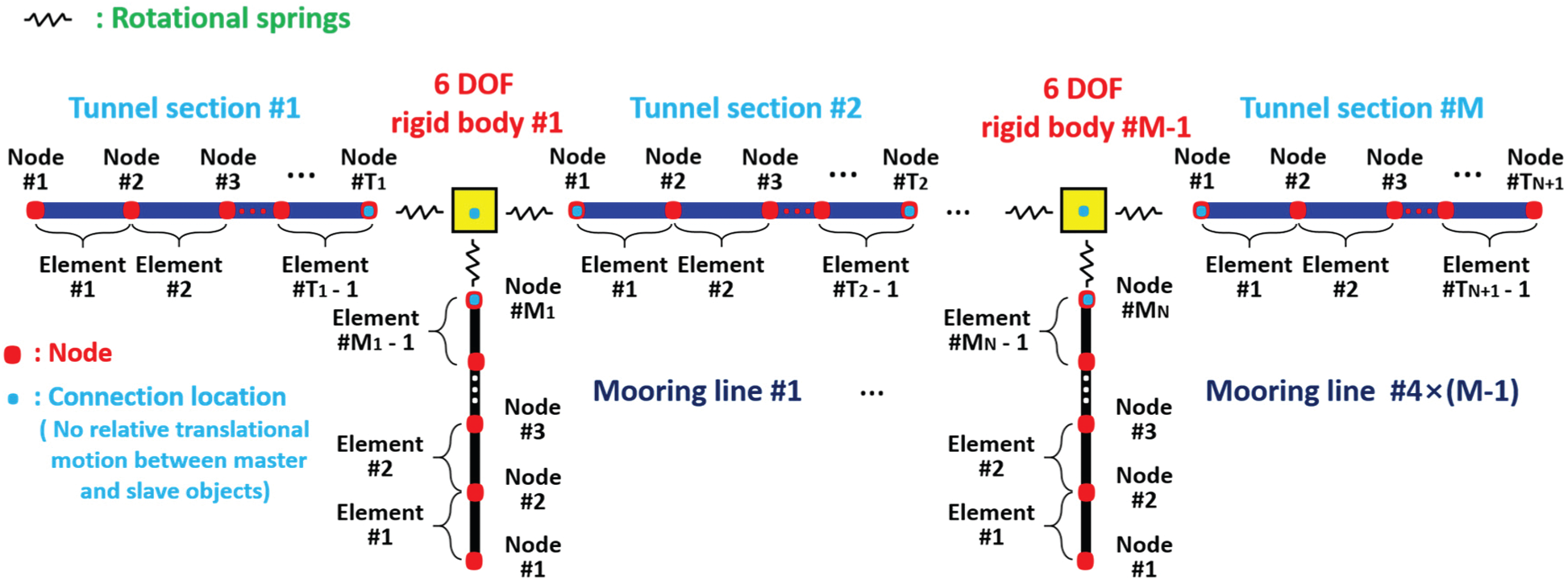
Figure 3: Coupling methodology [10]

The earthquake effect is considered by inputting the time histories of seismic lateral and vertical displacements at each anchor location of the mooring line and both ends of the tunnel. The seismic effect then appears on the tunnel through FC from mooring lines to the tunnel at the connection locations and Kx from tunnel ends to central locations through structural beams. In this case, the fluid kinematics is not considered in the earthquake problem although there may be minor effects from the corresponding seaquake; therefore, the hydrodynamic force on the structure is purely based on SFT's velocity and acceleration along its geometric center.

The present numerical simulation model has been validated against several experimental results in wave tanks [27,28].

3  Configuration and System Parameters

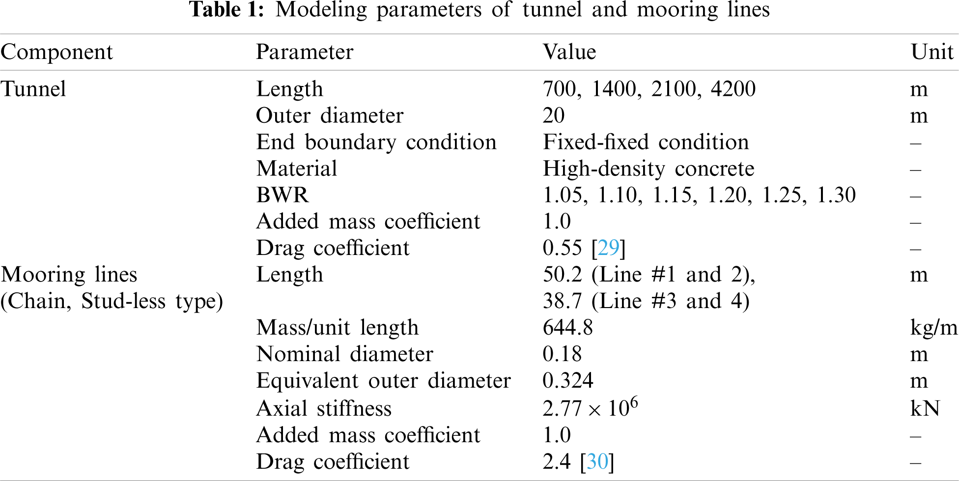
SFT's basic configuration and design parameters are shown in Fig. 1 and Tab. 1. SFT consists of 14 tunnel sections, 13 dummy rigid bodies, and 52 mooring lines, and thus 66 line models and 13 dummy rigid bodies are employed. The tunnel is made of concrete and has a diameter of 20 m. The fixed-fixed boundary condition is modeled at both ends representing bottom-fixed stations where there are no displacements and angles in 3D at both ends. In general, the distance between stations is longer than 2 km as an example of the subway station; however, a shorter interval may be needed for SFT application since they can be utilized for underwater evacuation and ventilation. The added mass coefficient is 1.0 due to a fully-submerged cylindrical shape [26]. The drag coefficient is 0.55, based on the experimental results at the cylinder's representative Reynold number and surface roughness [29]. Several system parameters are selected to conduct parametric studies. First, BWRs of 1.05–1.3 are selected to check the importance of static and dynamic tension. The tunnel's inner diameter is changed according to different BWRs by neglecting inner compartments for simplicity, which can be considered as an equivalent cross section. Then, the structural stiffness can be calculated from outer and inner diameters. Second, water depths are set as 100, 120, and 140 m: the corresponding submergence depths are changed to 61.5, 81.5, and 101.5 m by having the same mooring style and length. This is to investigate the relationship between global performance and submergence depth under wave excitations. The submergence depth is defined as the vertical distance between the water surface and the tunnel center. Third, four different tunnel lengths of 700, 1400, 2100, and 4200 m are taken into consideration: the corresponding mooring intervals are 50, 100, 150, and 300 m. The increased mooring interval results in reduced natural frequencies but increased static mooring tensions. Intuitively, at larger submergence depths, wave force is significantly reduced, and then sparse mooring interval may be used to save mooring-anchor and installation costs. An element length of 10 m is selected after convergence tests by comparing natural frequencies between different element lengths. For example, the 700 m long tunnel has 70 finite elements, sufficiently representing its elastic behaviors.

Studless chain mooring is chosen with a nominal diameter of 0.18 m, which is one of the largest sizes to handle large static and dynamic tensions. A mooring group consists of four mooring lines at the given tunnel cross section, and they are 60° inclined to the seabed. The same mooring group is distributed with equal interval along the tunnel length (see Fig. 1). The seabed is assumed to be flat with equal water depth. In the Morison formula for mooring lines, the added mass coefficient is 1.0 with its equivalent outer diameter of 0.324 m (1.8 times the nominal diameter), and the drag coefficient is 2.4 with its nominal diameter. The selections of the diameters and added mass and drag coefficients in the Morison equation are based on suggestions by the DNV Standard and OrcaFlex manual [25,30]. Based on the chain mooring line's characteristics, the axial stiffness term is only considered, whereas the bending and torsional effects are neglected. Mooring lines are modeled by eight equal-length elements to present their flexibility.

4  Environmental Conditions

Waves and earthquakes are considered as environmental conditions. The JONSWAP wave spectrum is utilized to produce the time histories of random waves. As shown in Fig. 4, two different random waves are generated: HSs are 11.7 and 3 m, regarded as 100-year storm conditions in the South Sea of Korea and a fjord in Norway. The corresponding TPs are 13 and 6 s, respectively. The peak enhancement parameters are selected to be 2.14 and 3.3 based on the references on the target sites [31,32]. The imposed JONSWAP spectrum is a representative one in a wide area of the South Sea of Korea, so it is independently applied to respective regions of three different water depths (100, 120, and 140 m), i.e., the transformation of a wave spectrum propagating over different water depths is not a concern in the present investigation. Two hundred sinusoids are superposed to generate random waves. The equal energy method in which each wave component has equal spectral energy is employed to avoid signal repetition for long time-series generation. 1-hour simulations are conducted for each wave condition to sufficiently represent statistic results. The time interval of time-domain simulations under wave excitations is 0.05 s. Wave direction is perpendicular to the tunnel length, as illustrated in Fig. 1 since this is to be the worst case.

Three real seismic displacements are collected from USGS in a magnitude range of 3.8–8.4 in the moment magnitude (MM) scale, as summarized in Tab. 2. The representative time histories and spectra, presented in Figs. 5–6, show that the larger the earthquake magnitude, the lower the dominant excitation frequency. This trend plays an essential role in SFT's dynamics associated with the system's natural frequencies. The time interval of seismic displacements and time-domain simulations is 0.005 s. The direction of earthquake propagation is assumed to be perpendicular to the tunnel length, and thus the same earthquake displacements without time delay are inputted to all anchor points of mooring lines and both ends of the tunnel.

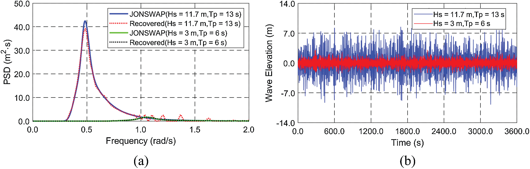
Figure 4: Spectra (input JONSWAP and recovered from time histories) (a) and time histories (b) of wave elevation

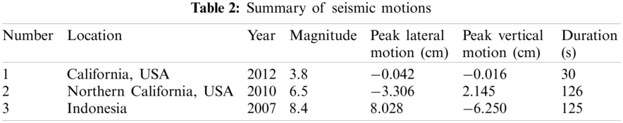
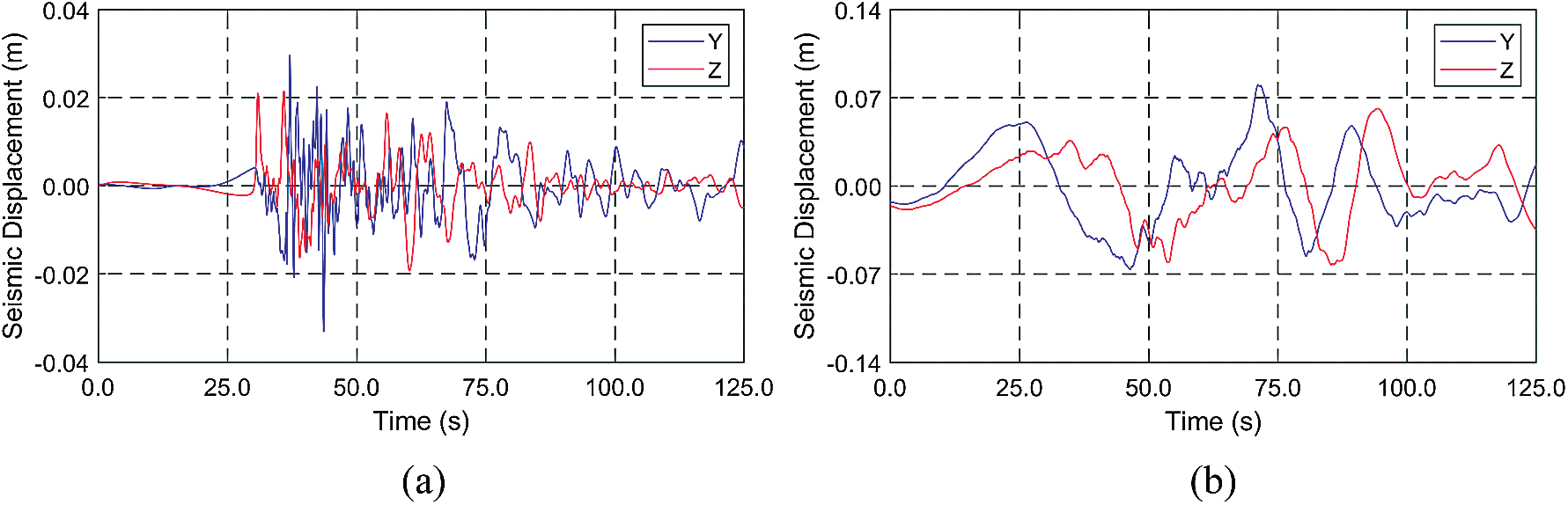
Figure 5: Time histories of seismic displacements (a) Northern California, USA, 2010 (magnitude = 6.5) (b) Indonesia, 2007 (magnitude = 8.4)

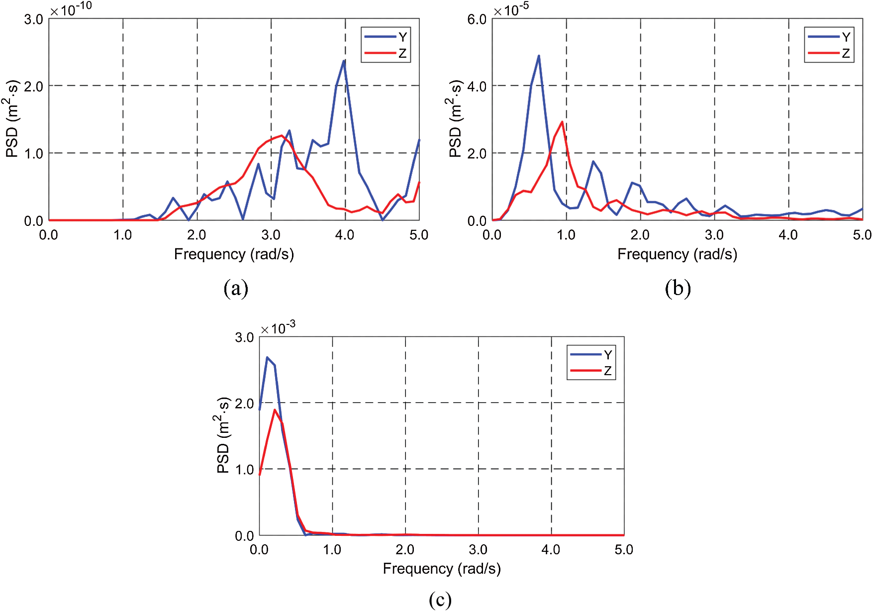
Figure 6: Spectra of seismic displacements (a) California, USA, 2012 (magnitude = 3.8) (b) Northern California, USA, 2010 (magnitude = 6.5) (c) Indonesia, 2007 (magnitude = 8.4)

5  Results and Discussions

5.1 Modal Analysis

Modal analysis is carried out to obtain the natural frequencies and mode shapes of the SFT contacting water after the static simulation. The representative model shapes and natural frequencies are presented in Fig. 7 and Tab. 3. The typical mode shapes with the fixed-fixed end-boundary conditions are obtained, including the effects of uniformly distributed mooring lines along the tunnel. The horizontal and vertical mode shapes are almost the same for the representative case. Whereas, the natural frequencies are different since the corresponding mooring stiffnesses are different for the given mooring-lines’ inclination angle. As can be seen in Tab. 3, the system's wet natural frequencies are not sensitive to the change of BWR. It is well-known that for the Euler-Bernoulli beam, the lowest natural frequency for the fixed-fixed boundary condition is represented as ωn=22.4EI/mL4, where EI is bending stiffness, m is mass per unit length, and L is tunnel length [33]. Therefore, the natural frequencies are significantly reduced by increasing the tunnel length and mooring interval, which can be an important consideration for reducing dynamic responses at the target environmental conditions. It is also interesting that the natural frequencies for the respective modes get closer to each other when tunnel length and mooring interval are increased.

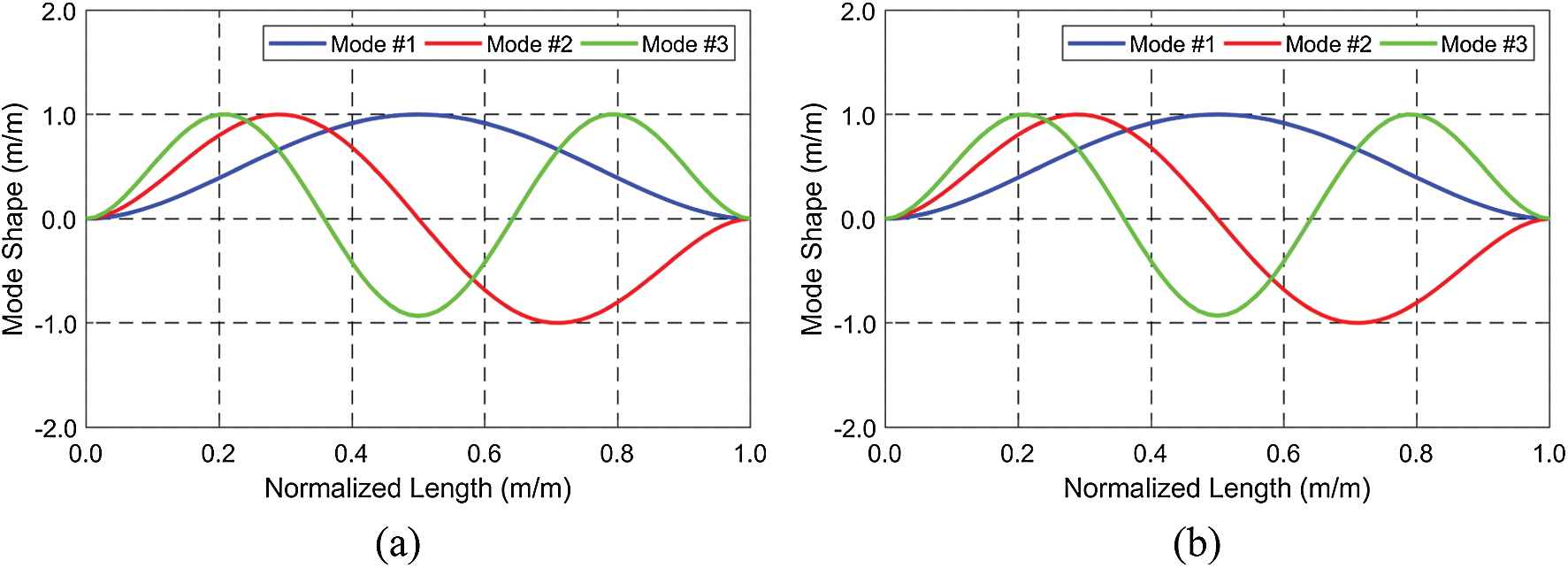
Figure 7: Horizontal (a) and vertical (b) mode shapes (tunnel length = 700 m, BWR = 1.3)

5.2 Dynamic Responses under Wave Excitations

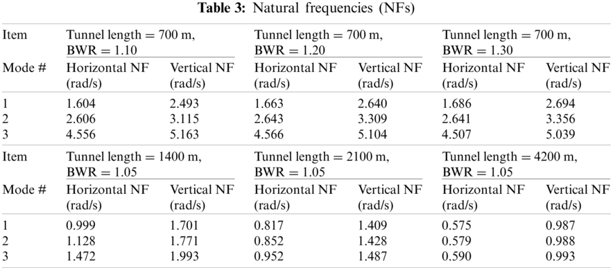
In this section, the tunnel's dynamic responses and mooring tensions are evaluated under wave excitations. As mentioned before, two different wave conditions (HS of 11.7 and 3 m) are selected: their corresponding TPS are 13 and 6 s. These wave conditions correspond to 100-year storm conditions in the South Sea of Korea and a Norwegian fjord. The sensitivity tests with respect to BWR, submergence depth, and tunnel length are performed to have a better engineering design at target wave conditions. Based on the authors’ previous studies, these parameters are very important for SFT design. The envelopes of the maximum and minimum displacements and maximum tensions are first checked to select major analysis locations, as shown in Fig. 8. The largest displacements and mooring tensions are observed at its mid-length. Also, the mooring tensions of Line #4 are the largest among four mooring lines while shorter mooring lines (Lines #3–#4) have higher mooring tensions than longer ones (Lines #1–#2). From this point, displacements at the mid-length and mooring tension of Line #4 at the mid-length are only presented since they are the largest.

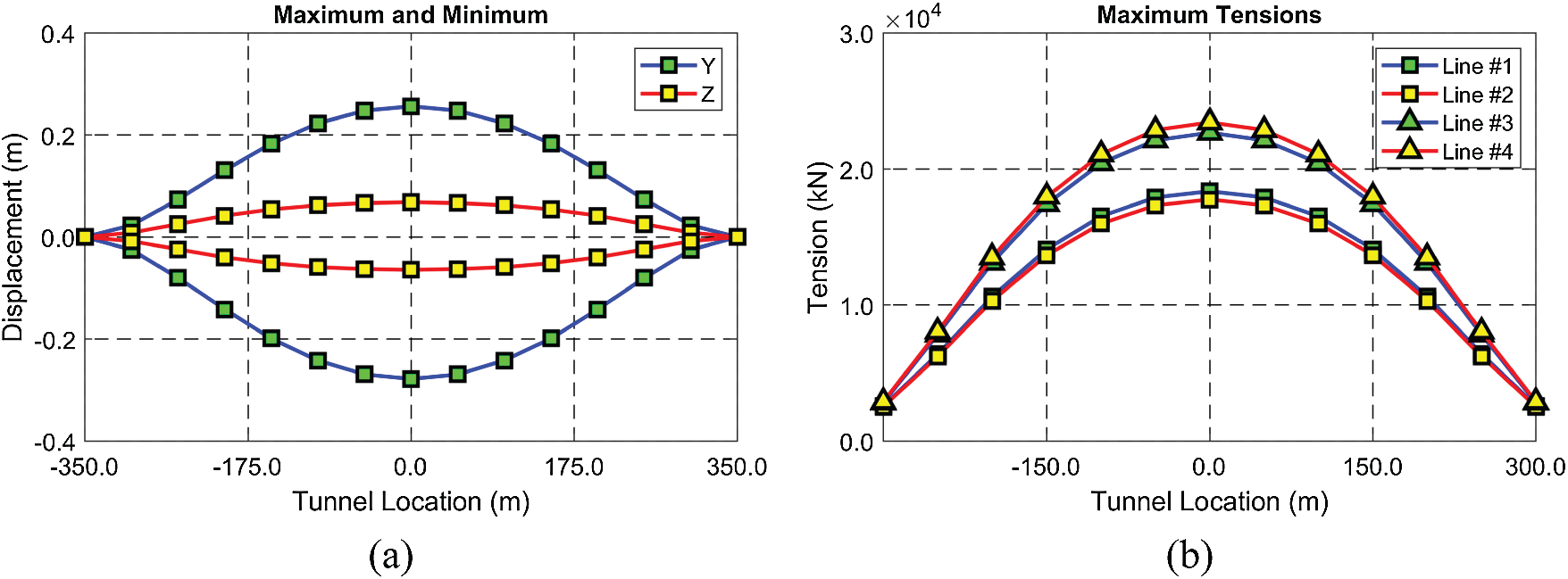
Figure 8: Envelopes of maximum and minimum displacements (a) and maximum mooring tensions (b) (BWR = 1.3, tunnel length = 700 m, submergence depth = 61.5 m)

First, BWR often plays a critical role in both static and dynamic responses, as demonstrated in Fig. 9. In this comparison, the tunnel length and submergence depth are fixed at 700 m (shortest) and 61.5 m (shallowest). In the severe wave condition (HS = 11.7 m), dynamic motions are lowest at the highest BWR of 1.3, and they significantly increase at BWR less than 1.15. The difference in natural frequencies among BWRs plays a relatively small role in dynamic responses since the differences are actually small and the lowest natural frequencies are far outside of TP. The dynamic responses are well limited at BWRs of 1.2–1.3, showing no noticeable difference. At lower BWR (1.05–1.15), the mooring snap loadings (happening just after being slack) mainly contribute to the sudden significant increase of SFT dynamics and mooring tensions, i.e., the smaller BWR, the larger dynamics. On the other hand, BWR mostly determines the static mooring tension such that small BWR results in smaller static mooring tension. The lower BWR is likely to produce the snap loading under the large wave force. Therefore, shallower submergence depth and/or bigger storm tend to induce more snap loading.

Figure 9: Standard deviations of displacements and their maxima and minima at different BWRs (submergence depth = 61.5 m) (a) HS = 11.7 m (b) HS = 11.7 m (c) HS = 3 m (d) HS = 3 m

Mooring tension further demonstrates the snap loading phenomenon, as can be seen in Fig. 10. The minimum mooring tensions at low BWR = 1.05–1.15 reach nearly zero (slack), then suddenly inducing large dynamic responses and mooring tensions by snap movement. This can further be supported by the time histories of tensions in Fig. 11. For this reason, the maximum mooring tensions at BWR = 1.05–1.15 are higher than those of BWR = 1.2–1.3 despite smaller static tensions. It is worth mentioning that BWR of 1.2 provides the smallest mooring tension because only minor snap loading is detected under moderate static mooring tension. As a result, the optimal BWR should be selected for the given submergence depth and wave excitation through this kind of investigation. Even for BWR = 1.2 with the given 50-m mooring interval, the maximum mooring tension is still higher than the allowable mooring load of 18376 kN (minimum breaking load (MBL) of 30689 kN for the Grade R5 chain divided by the safe factor (SF) of 1.67), which can be solved by a slightly shorter mooring interval.

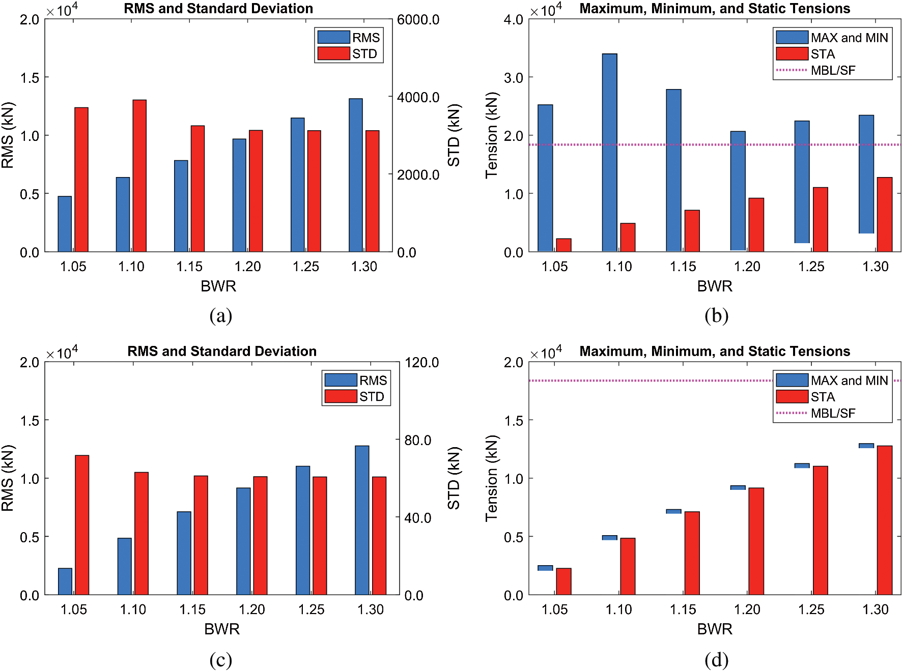
Figure 10: RMSs and standard deviations of tensions (Line #4), their maxima/minima, and static values at different BWRs (submergence depth = 61.5 m) (a) HS = 11.7 m (b) HS = 11.7 m (c) HS = 3 m (d) HS = 3 m

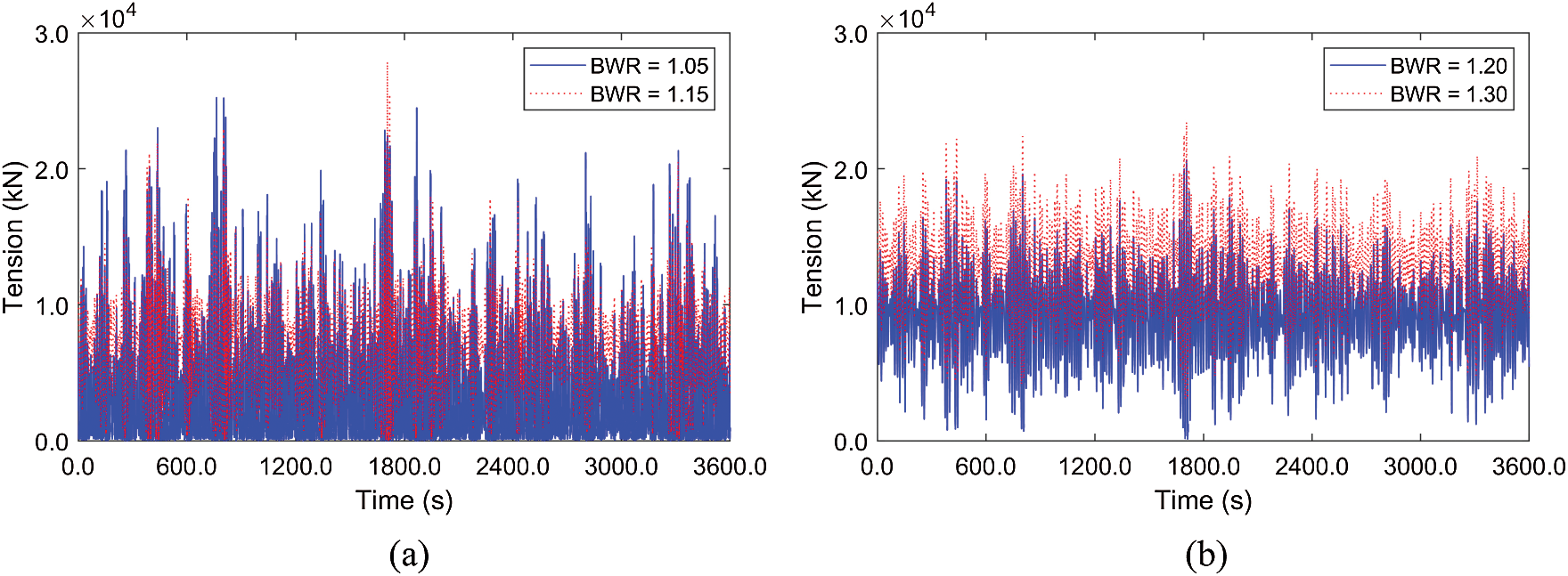
Figure 11: Time histories of mooring tensions (Line #4) at low (a) and high (b) BWRs (HS = 11.7 m, submergence depth = 61.5 m)

On the other hand, in the mild wave condition (HS = 3 m), no significant dynamic motions and tensions are observed regardless of BWRs due to the low wave force. Also, no snap loading is observed under this wave condition. In this case, the static mooring tension is a critical factor in mooring design, and thus the maximum tension is detected at the highest BWR of 1.3. As a result, BWR of 1.05 is the most promising solution governed by the static mooring tension. Based on the results under two different wave conditions, the lower BWR is beneficial under mild wave conditions since there is no snap loading and static mooring tension is low, while significant snap loadings must be solved under severe wave conditions by properly increasing BWR.

Second, the sensitivity with respect to submergence depth is checked, as shown in Figs. 12–13. In this comparison, only the severe wave condition (HS = 11.7 m) is considered under different submergence depths of 61.5, 81.5, and 101.5 m. Having the same mooring length, the submergence depths correspond to water depths of 100, 120, and 140 m. Note that the submergence depth is defined as the vertical distance between the sea surface and the tunnel's centerline. According to the wave theory, wave kinematics exponentially decay with submergence depth due to the term e−kz where k is wavenumber and z is submergence depth in deepwater. Such a trend is also observed in this sensitivity test. The larger the submergence depth, the smaller the dynamic responses (Fig. 12). The large displacements, detected at BWR = 1.1 and submergence depth = 61.5 m, are substantially reduced at larger submergence depths. The dynamic responses at BWRs of 1.2 and 1.3 are almost identical regardless of submergence depth. Based on the tension results (Fig. 13), the static mooring tension governs the RMS value, especially at large submergence depth, because dynamic motions and tensions are not that significant. At the submergence depth of 101.5 m, there is no difference in dynamic tensions among different BWRs since there is no snap loading, which results in the lowest maximum mooring tension at BWR = 1.1. It can be concluded that if the wave force is small, such as the cases of mild wave condition and sufficient submergence depth, smaller BWR is beneficial in reducing the maximum mooring tension through smaller static tension.

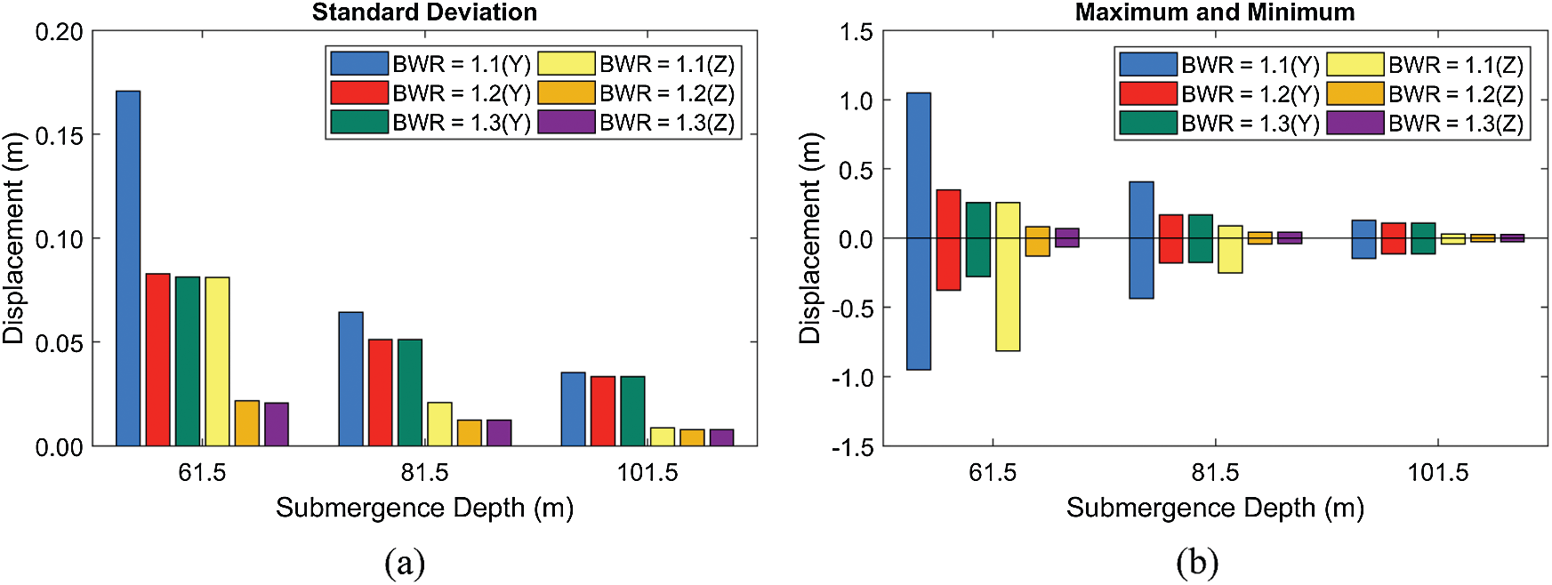
Figure 12: Standard deviations of displacements (a) and their maxima and minima (b) at different submergence depths and BWRs (HS = 11.7 m)

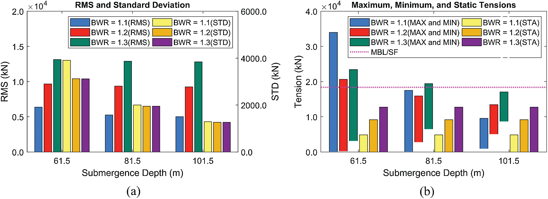
Figure 13: RMSs and standard deviations of tensions (Line #4) (a), their maxima/minima, and static values (b) at different submergence depths and BWRs (HS = 11.7 m)

Third, the effects of tunnel length and mooring interval on dynamic responses and mooring tensions are assessed, as shown in Figs. 14–15. In the previous two sensitivity tests, it is seen that the sharp increase of mooring tension is highly associated with snap loading. The snap loading does not occur when BWR and submergence depth are large enough. However, in terms of the maximum mooring tension, high BWR may be harmful due to high static tension. This trend is also reflected when we consider different tunnel lengths (i.e., mooring intervals). Here, BWR is fixed at 1.05 considering increased mooring interval and the corresponding increased burden to support more buoyancy per mooring. Fjord wave condition warrants that there is no snap loading even at low BWR = 1.05. Increasing tunnel length and mooring interval for the same number of mooring lines may substantially decrease mooring/anchor and their installation costs. In this regard, four different tunnel lengths (700, 1400, 2100, and 4200 m) are compared in the mild wave condition (HS = 3 m). They correspond to mooring intervals of 50, 100, 150, and 300 m. The rough wave condition has no room to consider larger mooring interval unless deeply submerged since the maximum mooring tension is already higher than the allowable tension. The longer the mooring interval, the larger the static tension on the individual line and lower the tunnel natural frequencies as becoming softer, as described in Section 5.1.

As shown in Figs. 14–15, the tunnel motions and mooring tensions are highly related to the natural frequencies. For example, the largest lateral and vertical responses are observed at the tunnel lengths of 2100 and 4200 m, respectively, at which the lowest lateral and vertical natural frequencies are close to the input peak frequency. Thus, those system parameters should carefully be selected to avoid resonant motions for the given design-storm condition at the target area. The tunnel length mainly determines the static mooring tension and its RMS value (Fig. 15). Although the static tension is higher at the longer tunnel length, the dynamic responses and tensions can be smaller for longer tunnel length (see the decrease of standard deviation from 2100 to 4200 m) due to the larger separation between tunnel natural frequency and peak of the incident wave. The tunnel length of 4200 m (= mooring interval 300 m) is possible even at 61.5 m submergence, and an even longer tunnel (and mooring interval) is also feasible at larger submergence depths.

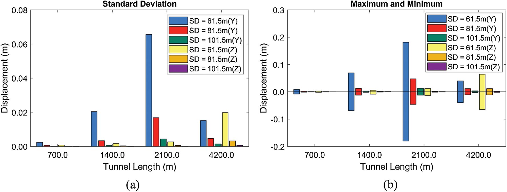
Figure 14: Standard deviations of displacements (a) and their maxima and minima (b) at different tunnel lengths and submergence depths (HS = 3 m, BWR = 1.05)

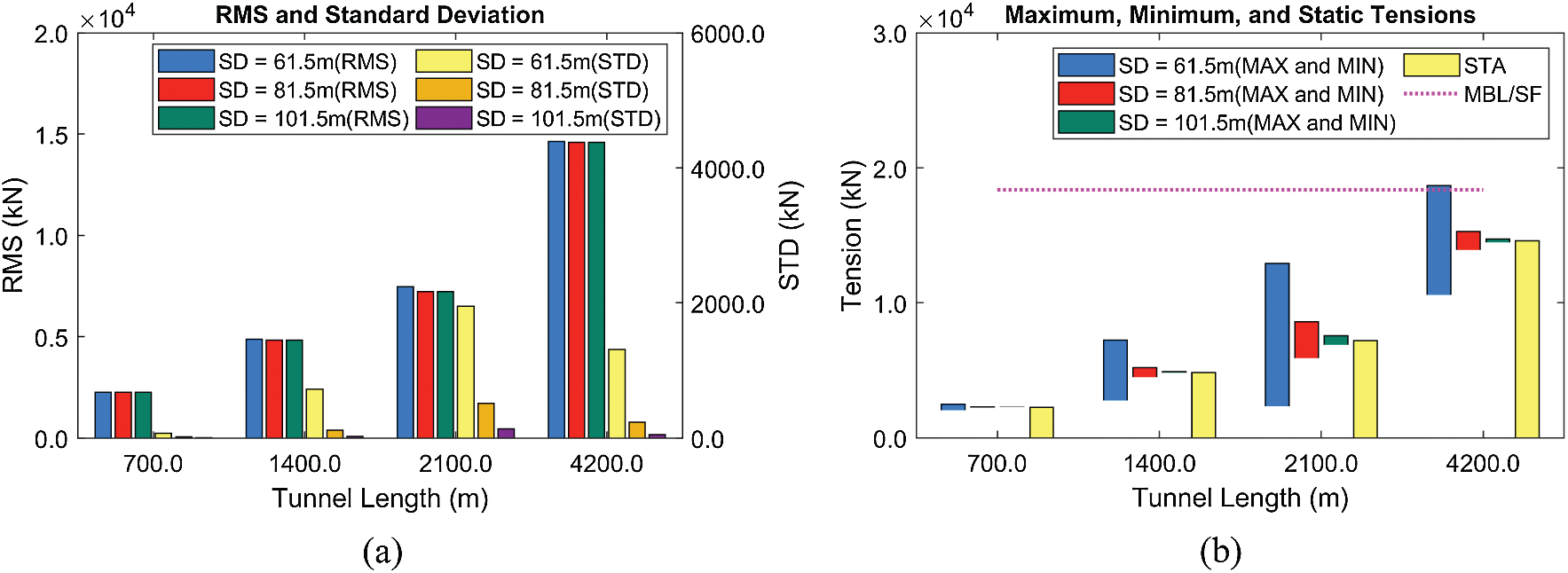
Figure 15: RMSs and standard deviations of tensions (Line #4) (a), their maxima/minima, and static values (b) at different tunnel lengths and submergence depths (HS = 3 m, BWR = 1.05)

5.3 Dynamic Responses under Earthquake Excitations

In this section, the tunnel's dynamic responses and the corresponding mooring tensions are evaluated under earthquake excitations. In the case of earthquake-induced dynamics, tunnel's submergence depth is almost irrelevant unless it is close to the free surface. Instead, mooring style and length become more relevant parameters. In this section, the submergence depth is fixed at 61.5 m. Three MM (moment magnitude)-scale time histories of earthquake excitations are obtained from USGS and employed in this study. Based on the spectral results in Fig. 6, the higher the earthquake magnitude, the lower the peak excitation frequency. Thus, it is very important to predefine the possible earthquake range to minimize the resulting motion. Sensitivity tests with varying BWRs and tunnel lengths are performed to better understand the earthquake-proof engineering design at the target earthquake excitations.

First, the influences of BWR and earthquake magnitudes on dynamic responses and mooring tensions are checked, as reported in Figs. 16–17. As shown in Fig. 16, both earthquake magnitude and dominant seismic frequency play important roles in dynamics responses. When the earthquake magnitude is 3.8, the resulting dynamic responses are negligible due to the small earthquake displacements and the dominant earthquake frequencies far apart from the tunnel's lowest natural frequencies. However, as the dominant earthquake frequency of MM = 6.5 gets close to the tunnel's lowest natural frequency, large resonant motions are observed, as in Fig. 16. The largest earthquake with magnitude = 8.4 also induces large dynamic motions, but the increase is not so large compared to the 6.5 case considering that the MM scale is log scale (8.4 case is 78 times larger in earthquake moment than 6.5 case). That is because the dominant seismic frequency of MM = 8.4 is farther apart from the lowest natural frequency of tunnel than MM = 6.5 case. Interestingly, despite the increase in dynamic motions from MM = 6.5 to 8.4, there is little increase in mooring tension. This is due to that when the horizontal motion is maximum, the vertical motion is almost zero and vice versa. Also, the BWR variation induces some motion variations mainly due to the changes in the tunnel's natural frequencies. The low BWR can reduce the earthquake-induced dynamic motions because the earthquake movements are less directly transmitted to the tunnel as mooring lines become less taut.

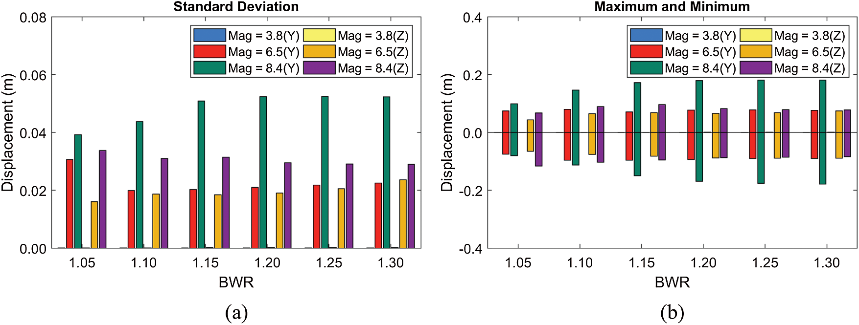
Figure 16: Standard deviations of displacements (a) and their maxima and minima (b) at different BWRs (submergence depth = 61.5 m)

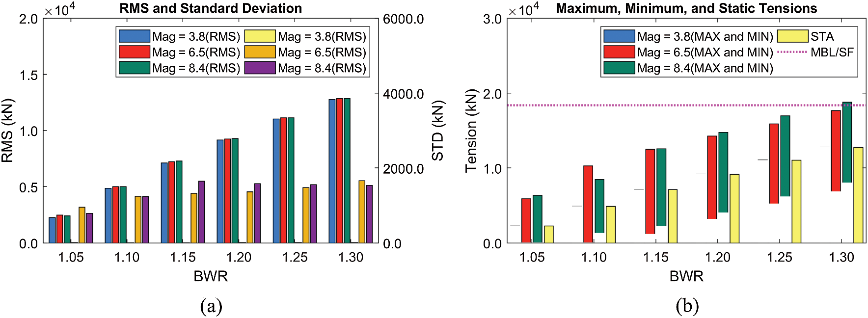
Figure 17: RMSs and standard deviations of tensions (Line #4) (a), their maxima/minima, and static values (b) at different BWRs (submergence depth = 61.5 m)

As for the mooring tension, the maximum tension is governed by the static mooring tension, as shown in Fig. 17. For example, the dynamic tension is negligible at the earthquake magnitude of 3.8. In this case, the static tension plays a leading role in the mooring design, and lower BWR is better because of low static tension. The same trend is also observed at higher seismic magnitudes. As a result, the lower BWR is beneficial under seismic excitations unless significant snap loading is detected. As pointed out earlier, the mooring tensions at MM = 6.5 and 8.4 are similar although the seismic displacements at MM = 6.5 are much smaller than MM = 8.4, demonstrating the importance of properly locating the system's natural frequencies against the design earthquake condition.

Finally, the sensitivity test with respect to the tunnel length is carried out, as presented in Figs. 18–19. Again, the tunnel length (and mooring interval) is a critical factor in anchor-system installation, in which the cost and difficulty are significantly reduced as the tunnel length and mooring interval are increased mainly due to the decreased total number of anchors and mooring lines. In this comparison, BWR is fixed to be 1.05 to see the SFT dynamics under low static tension. As shown in Fig. 18, the smallest earthquake induces little SFT dynamics compared to higher earthquakes, regardless of the tunnel length. Moreover, the importance of the location of natural frequencies can be observed. The MM = 6.5 earthquake spectral energy (Fig. 6) at the lowest resonance frequencies (Tab. 3 for BWR = 1.05) is considerable, and thus the corresponding tunnel motion is as large as that of much larger earthquake MM = 8.4. For the latter, the peak earthquake frequency is farther away from the tunnel's lowest natural frequencies, and thus the corresponding tunnel motions are not large. Therefore, the SFT's natural frequencies should be carefully adjusted in the design stage to minimize the earthquake-induced tunnel motions and mooring tensions. In Fig. 19, even for the largest tunnel length of 4200 m and mooring interval of 300 m, the mooring can satisfy the safety factor even at the largest earthquake of MM = 8.4, i.e., the construction cost can significantly be saved. When earthquake frequency is away from the system's lowest natural frequencies, we can significantly extend the mooring interval with low BWR. The potential snap loading on mooring still needs to be carefully checked by the tunnel-mooring-coupled dynamics computer simulation program.

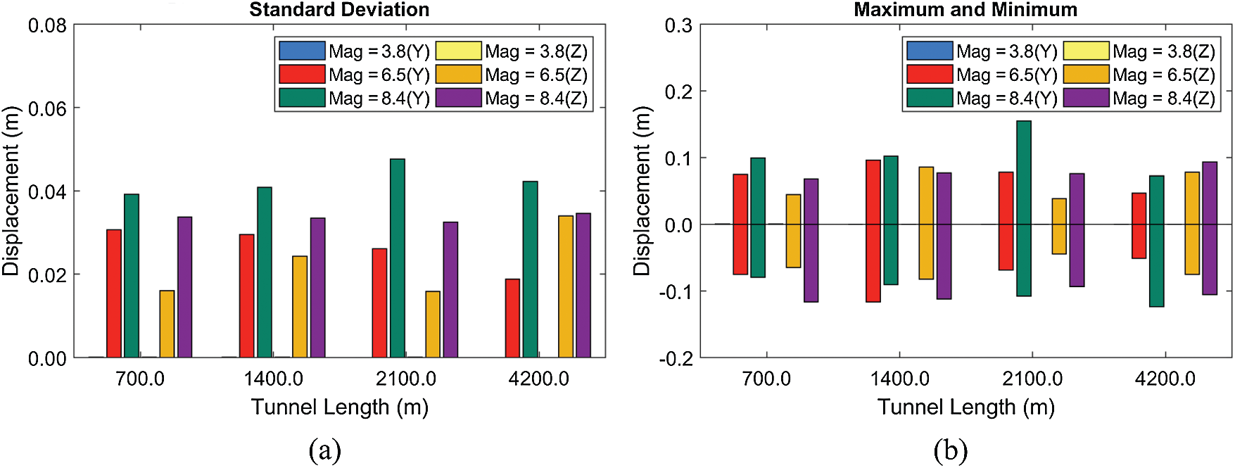
Figure 18: Standard deviations of displacements (a) and their maxima and minima (b) at different tunnel lengths (BWR = 1.05, submergence depth = 61.5 m)

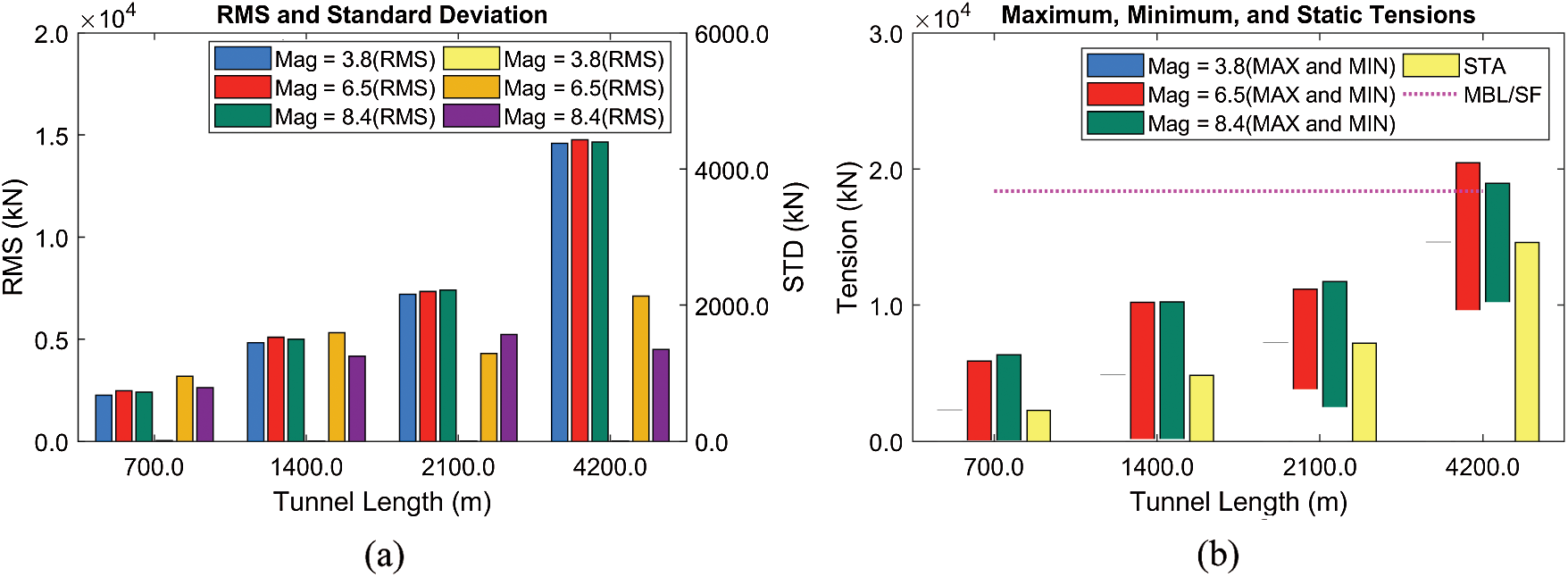
Figure 19: RMSs and standard deviations of tensions (Line #4) (a), their maxima/minima, and static values (b) at different tunnel lengths (BWR = 1.05, submergence depth = 61.5 m)

From the comparison between the 100-year storm condition in South Korea (HS = 11.7 m) and the largest earthquake (MM = 8.4), the 100-year storm condition induces larger displacements and maximum mooring tension. Also, waves induce steady-state responses all year long, whereas earthquakes induce transient responses for a short time [10]. In this regard, wave excitations are a more dominant factor for the present SFT design, while earthquake excitations play some roles in the structural design.

6  Conclusions

In this study, the practical design strategy for a large size SFT is investigated. A coupled time-domain dynamics simulation model for SFT is built considering wave and earthquake excitations. Tunnel and mooring lines are modeled by using a series of the finite-element line model. The line theory is based on a lumped mass method, where physical components are all lumped at nodes and they are connected by massless linear springs to represent elastic behaviors. The dummy-connection-mass method and the constraint boundary conditions are utilized to couple the tunnel and mooring lines. The Morison equation is employed to estimate the wave- and earthquake-induced hydrodynamic forces at instantaneous node positions. Various wave and earthquake conditions are tested to check the corresponding dynamic motions and mooring tensions at different system parameters. The wet natural frequencies are obtained through modal analysis for different BWRs, tunnel lengths, and mooring intervals. Systematic parametric studies are conducted under different BWRs, submergence depths, and tunnel lengths (and mooring interval) to build a cost-effective design strategy while satisfying the allowable mooring tension. The following design strategies are established according to the simulation results:

•   The primary wet natural frequencies with mooring need to be adjusted depending on the target wave and earthquake conditions to reduce the resonant motions.

•   Reducing BWR is generally beneficial when the dynamic environmental load is relatively small. In this case, the maximum tension is governed by the static tension by BWR. However, the possibility of snap loading at low BWRs should be carefully examined from the simulation.

•   The tunnel length or mooring interval can significantly be extended with increasing submergence depth since wave excitations decay exponentially with submergence depth.

•   The tunnel length or mooring interval can also be extended with appropriate BWR as storm-wave and seabed-earthquake conditions are relatively mild. In this case, the high static tension can be reduced with smaller BWR while dynamic tension plays relatively a minor role.

•   In the case of 100-yr severe storm condition at the South Sea of Korea, with 61.5-m submergence depth and 50-m mooring interval, BWR = 1.2 turns out to be the best case satisfying the mooring tension requirement. At a larger submergence depth of 101.5 m, no snap loading is observed, and the tension is governed by the static tension. In the case of 100-year storm at submergence depth 61.5 m of Norwegian Fjord or Indonesian earthquake of magnitude 8.4, tunnel length between two fixed stations as large as 4200 m (or mooring interval as large as 300 m) can be used with BWR = 1.05.

Funding Statement: This work was supported by the National Research Foundation of Korea (NRF) Grant funded by the Korean Government (MSIT) (No. 2017R1A5A1014883).

Conflicts of Interest: The authors declare that they have no conflicts of interest to report regarding the present study.

References

 1.  Remseth, S., Leira, B. J., Okstad, K. M., Mathisen, K. M., Haukås, T. (1999). Dynamic response and fluid/structure interaction of submerged floating tunnels. Computers & Structures, 72, 659–685. DOI 10.1016/S0045-7949(98)00329-0. [Google Scholar] [CrossRef]

 2.  Oh, S., Park, W., Jang, S., Kim, D., Ahn, H. (2013). Physical experiments on the hydrodynamic response of submerged floating tunnel against the wave action. Proceedings of the 7th International Conference on Asian and Pacific Coasts (APAC 2013pp. 582–587. Bali, Indonesia. [Google Scholar]

 3.  Seo, S. I., Mun, H. S., Lee, J. H., Kim, J. H. (2015). Simplified analysis for estimation of the behavior of a submerged floating tunnel in waves and experimental verification. Marine Structures, 44, 142–158. DOI 10.1016/j.marstruc.2015.09.002. [Google Scholar] [CrossRef]

 4.  Yang, Z., Li, J., Zhang, H., Yuan, C., Yang, H. (2020). Experimental study on 2D motion characteristics of submerged floating tunnel in waves. Journal of Marine Science and Engineering, 8, 123. DOI 10.3390/jmse8020123. [Google Scholar] [CrossRef]

 5.  Deng, S., Ren, H., Xu, Y., Fu, S., Moan, T. et al. (2020). Experimental study of vortex-induced vibration of a twin-tube submerged floating tunnel segment model. Journal of Fluids and Structures, 94, 102908. DOI 10.1016/j.jfluidstructs.2020.102908. [Google Scholar] [CrossRef]

 6.  Jin, C., Kim, M. H. (2020). Tunnel-mooring-train coupled dynamic analysis for submerged floating tunnel under wave excitations. Applied Ocean Research, 94, 102008. DOI 10.1016/j.apor.2019.102008. [Google Scholar] [CrossRef]

 7.  Won, D., Seo, J., Kim, S., Park, W. S. (2019). Hydrodynamic behavior of submerged floating tunnels with suspension cables and towers under irregular waves. Applied Sciences, 9, 5494. DOI 10.3390/app9245494. [Google Scholar] [CrossRef]

 8.  Chen, Z., Xiang, Y., Lin, H., Yang, Y. (2018). Coupled vibration analysis of submerged floating tunnel system in wave and current. Applied Sciences, 8, 1311. DOI 10.3390/app8081311. [Google Scholar] [CrossRef]

 9.  Muhammad, N., Ullah, Z., Choi, D. H. (2017). Performance evaluation of submerged floating tunnel subjected to hydrodynamic and seismic excitations. Applied Sciences, 7, 1122. DOI 10.3390/app7111122. [Google Scholar] [CrossRef]

10. Jin, C., Bakti, F. P., Kim, M. (2021). Time-domain coupled dynamic simulation for SFT-mooring-train interaction in waves and earthquakes. Marine Structures, 75, 102883. DOI 10.1016/j.marstruc.2020.102883. [Google Scholar] [CrossRef]

11. Kim, K. H., Bang, J. S., Kim, J. H., Kim, Y., Kim, S. J. et al. (2013). Fully coupled BEM-fEM analysis for ship hydroelasticity in waves. Marine Structures, 33, 71–99. DOI 10.1016/j.marstruc.2013.04.004. [Google Scholar] [CrossRef]

12. Das, S., Cheung, K. F. (2012). Hydroelasticity of marine vessels advancing in a seaway. Journal of Fluids and Structures, 34, 271–290. DOI 10.1016/j.jfluidstructs.2012.05.015. [Google Scholar] [CrossRef]

13. Newman, J. N. (1994). Wave effects on deformable bodies. Applied Ocean Research, 16, 47–59. DOI 10.1016/0141-1187(94)90013-2. [Google Scholar] [CrossRef]

14. Lu, D., Fu, S., Zhang, X., Guo, F., Gao, Y. (2016). A method to estimate the hydroelastic behaviour of VLFS based on multi-rigid-body dynamics and beam bending. Ships and Offshore Structures, 14, 354–362. DOI 10.1080/17445302.2016.1186332. [Google Scholar] [CrossRef]

15. Bakti, F. P., Jin, C., Kim, M. H. (2021). Practical approach of linear hydro-elasticity effect on vessel with forward speed in the frequency domain. Journal of Fluids and Structures, 101, 103204. DOI 10.1016/j.jfluidstructs.2020.103204. [Google Scholar] [CrossRef]

16. Lu, W., Ge, F., Wang, L., Wu, X., Hong, Y. (2011). On the slack phenomena and snap force in tethers of submerged floating tunnels under wave conditions. Marine Structures, 24, 358–376. DOI 10.1016/j.marstruc.2011.05.003. [Google Scholar] [CrossRef]

17. Sharma, M., Kaligatla, R., Sahoo, T. (2020). Wave interaction with a submerged floating tunnel in the presence of a bottom mounted submerged porous breakwater. Applied Ocean Research, 96, 102069. DOI 10.1016/j.apor.2020.102069. [Google Scholar] [CrossRef]

18. Jin, R., Gou, Y., Geng, B., Zhang, H., Liu, Y. (2020). Coupled dynamic analysis for wave action on a tension leg-type submerged floating tunnel in time domain. Ocean Engineering, 212, 107600. DOI 10.1016/j.oceaneng.2020.107600. [Google Scholar] [CrossRef]

19. Yarramsetty, P. C. R., Domala, V., Poluraju, P., Sharma, R. (2019). A study on response analysis of submerged floating tunnel with linear and nonlinear cables. Ocean Systems Engineering, 9, 219–240. DOI 10.12989/ose.2019.9.3.219. [Google Scholar] [CrossRef]

20. Di Pilato, M., Perotti, F., Fogazzi, P. (2008). 3D dynamic response of submerged floating tunnels under seismic and hydrodynamic excitation. Engineering Structures, 30, 268–281. DOI 10.1016/j.engstruct.2007.04.001. [Google Scholar] [CrossRef]

21. Xie, J., Chen, J. (2021). Dynamic response analysis of submerged floating tunnel-canyon water system under earthquakes. Applied Mathematical Modelling, 94, 757–779. DOI 10.1016/j.apm.2021.01.031. [Google Scholar] [CrossRef]

22. Lee, J. H., Seo, S. I., Mun, H. S. (2016). Seismic behaviors of a floating submerged tunnel with a rectangular cross-section. Ocean Engineering, 127, 32–47. DOI 10.1016/j.oceaneng.2016.09.033. [Google Scholar] [CrossRef]

23. Martinelli, L., Barbella, G., Feriani, A. (2011). A numerical procedure for simulating the multi-support seismic response of submerged floating tunnels anchored by cables. Engineering Structures, 33, 2850–2860. DOI 10.1016/j.engstruct.2011.06.009. [Google Scholar] [CrossRef]

24. Jin, C., Kim, M. H. (2018). Time-domain hydro-elastic analysis of a SFT (submerged floating tunnel) with mooring lines under extreme wave and seismic excitations. Applied Sciences, 8, 2386. DOI 10.3390/app8122386. [Google Scholar] [CrossRef]

25. Orcina, Ltd (2018). OrcaFlex manual. Daltongate Ulverston Cumbria, UK. [Google Scholar]

26. Faltinsen, O. (1993). Sea loads on ships and offshore structures. London, UK: Cambridge University Press. [Google Scholar]

27. Lee, J., Jin, C., Kim, M. (2017). Dynamic response analysis of submerged floating tunnels by wave and seismic excitations. Ocean Systems Engineering, 7, 1–19. DOI 10.12989/ose.2017.7.1.001. [Google Scholar] [CrossRef]

28. Cifuentes, C., Kim, S., Kim, M., Park, W. (2015). Numerical simulation of the coupled dynamic response of a submerged floating tunnel with mooring lines in regular waves. Ocean Systems Engineering, 5, 109–123. DOI 10.12989/ose.2015.5.2.109. [Google Scholar] [CrossRef]

29. Thompson, N. (1980). Mean forces, pressure and flow field velocities for circular cylindrical structures: Single cylinder with two-dimensional flow. EDU Data Item, 80025. [Google Scholar]

30. Veritas, D. N. (2010). Offshore standard DNV-OS-E301: Offshore standard-position mooring, Høvik, Norway: Det Norske Veritas (DNV) Oslo. [Google Scholar]

31. Suh, K. D., Kwon, H. D., Lee, D. Y. (2010). Some statistical characteristics of large deepwater waves around the Korean peninsula. Coastal Engineering, 57, 375–384. DOI 10.1016/j.coastaleng.2009.10.016. [Google Scholar] [CrossRef]

32. Sha, Y., Amdahl, J., Aalberg, A., Yu, Z. (2018). Numerical investigations of the dynamic response of a floating bridge under environmental loadings. Ships and Offshore Structures, 13, 113–126. DOI 10.1080/17445302.2018.1426818. [Google Scholar] [CrossRef]

33. Rao, S. S. (2007). Vibration of continuous systems. Hoboken, New Jesey, USA: John Wiley & Sons, Inc. [Google Scholar]

Appendix A: Formulations of Structural Stiffness Force for Line Model

As given in Eq. (1) and Fig. 2, Kx describes the structural deformability with axial, bending, and torsional springs. The detailed explanation is also available in [25]. Tension is first estimated by the axial spring at the center of each element. The effective tension is calculated as:

Te=Tw+(poa0−piai)(A1)

where Tw is the wall tension, and p and a are the pressure and cross-sectional area with subscripts o and i denoting external and internal. Tw is computed as:

Tw=EAε−2ν(poa0−piai)+kttτl0(A2)

where EA is the axial stiffness, ε is the axial strain, ν is the Poisson ratio, ktt is the tension-torsion coupling coefficient, τ is the torsional angle, l0 and is the unstretched element length. The bending moment magnitude is then computed by the bending springs at either side of the node as:

|m|=EI|c|(A3)

where EI is the bending stiffness, and c is the curvature. The bending moment is in the binormal direction. The shear force is then calculated at both ends of the segment with the calculated bending moments at either side of the node as:

fs=sz×1l(m2−m1)(A4)

where sz is the element's axial direction, and l is the instantaneous element length. The torsional moment magnitude is finally evaluated at the center of each element as:

|mx|=kτl0+kttε(A5)

where k the is torsional stiffness. The torsional moment is in the element axial direction. After all the calculations are done, these components are combined with other non-structural loads such as weight and wave forces to estimate the total force on each node.

Appendix B: Dummy-Connection-Mass Method

The dummy-connection-mass method [6,10,24] was developed to couple several line models for the SFT study. The tunnel and mooring lines are modeled with separate line models, as illustrated in Fig. 3. The tunnel is divided into M tunnel sections, and M−1 dummy rigid bodies are positioned with rotational springs between all connection locations. For a simple problem with a dummy rigid body and line, the structural stiffness force Kx and constraint force FC can be established, as shown in Fig. B1. For translational motions, Node 1's 3D translational displacements are the same as the rigid body's ones (blue boxes in Fig. B1), which is called the constraint condition. Node 1's translational DOFs are not needed to be solved and eliminated (yellow box) since its displacements are already defined based on the constraint condition. The interaction between rigid body and Node 1 influences Node 2's dynamic motions through the Nodes 1–2 coupling matrix (gray box). These terms move to the right-hand side to be FC. Similarly, FC on the rigid body is established as a form of contact force (purple box). For rotational motions, 3D rotational springs are located between the rigid body and Node 1, and the body-Node 1 coupling matrix is generated (green boxes), which moves to the right-hand side to be FC. The proposed numerical model was systematically validated with another numerical simulation program in the previous studies under wave, earthquake, and moving vehicle loads [10,24].

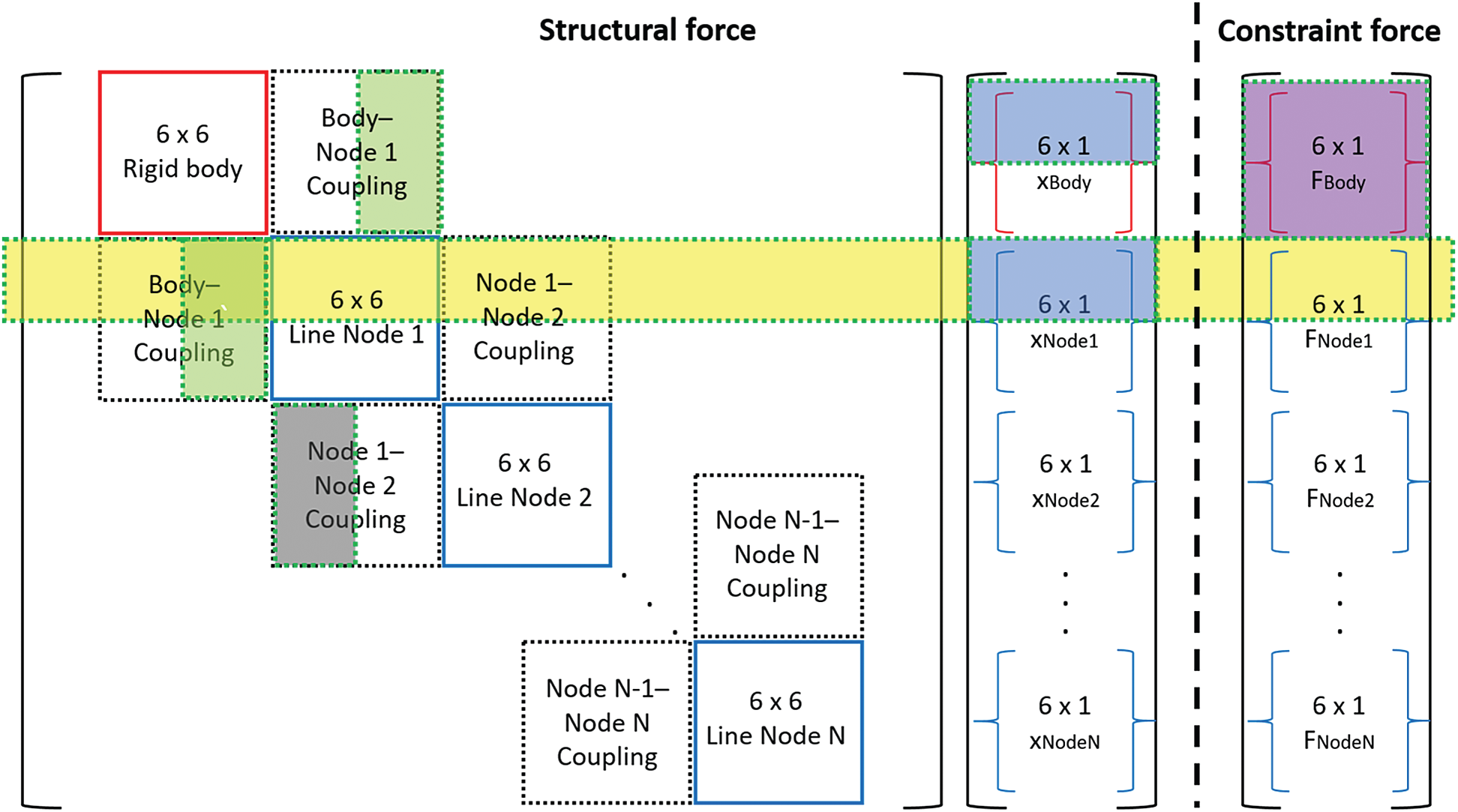
Figure B1: Structural stiffness and constraint forces for body-line interaction

This work is licensed under a Creative Commons Attribution 4.0 International License, which permits unrestricted use, distribution, and reproduction in any medium, provided the original work is properly cited.