Computer Modeling in Engineering & Sciences

DOI: 10.32604/cmes.2021.015549

ARTICLE

Computational Analysis of Airflow in Upper Airway under Light and Heavy Breathing Conditions for a Realistic Patient Having Obstructive Sleep Apnea

W. M. Faizal1,2, N. N. N. Ghazali2,*, C. Y. Khor1, M. Z. Zainon2, Irfan Anjum Badruddin3,4,*, Sarfaraz Kamangar4, Norliza Binti Ibrahim5 and Roziana Mohd Razi6

1Faculty of Mechanical Engineering Technology, University Malaysia Perlis, Perlis, Malaysia
2Department of Mechanical Engineering, Faculty of Engineering, University of Malaya, Kuala Lumpur, 50603, Malaysia
3Research Center for Advanced Materials Science, King Khalid University, Abha, 61413, Saudi Arabia
4Department of Mechanical Engineering, College of Engineering, King Khalid University, Abha, 61421, Saudi Arabia
5Department of Oral & Maxillofacial Clinical Science, Faculty of Dentistry, University of Malaya, Kuala Lumpur, 50603, Malaysia
6Department of Paediatric Dentistry and Orthodontics, Faculty of Dentistry, University of Malaya, Kuala Lumpur, 50603, Malaysia
*Corresponding Authors: N. N. N. Ghazali. Email: nik_nazri@um.edu.my; Irfan Anjum Badruddin. Email: magami.irfan@gmail.com
Received: 26 December 2020; Accepted: 20 April 2021

1  Introduction

Obstructive sleep apnea has affected many people across the globe and has a tendency to decrease quality of life by leading to other health issues [1]. Sleep apnea is considered as an underdiagnosed disease, which can lead to various adverse effects [2]. In order to assist clinicians to make the best decision, researchers are adopting various techniques to evaluate and understand the phenomenon of airflow in the human respiratory system; this could shed light on sleep apnea. The rapid advancement of medical imaging technology and three-dimensional modelling techniques has facilitated the numerical study of the airflow in the human upper airway while considering the real features of a patient. With the aid of methods such as computational fluid dynamics (CFD), the understanding of the airflow phenomena in the human upper airway during inhalation and exhalation has improved [3]. Additionally, particle transport and deposition of the human upper airway can be simulated in the realistic simulation model. The CFD simulation provides detailed results in terms of local and global airflow parameters and properties [4]. For example, airflow velocity, pressure drop, vortices, particle deposition and skin friction coefficient of the human upper airway can be obtained from the CFD results.

The airflow in the airways can behave in turbulent manner, which undergoes irregular fluctuations. The speed of the turbulent flow at a point always changes in terms of magnitude and direction [5]. The intensity of the turbulence is called Turbulence Kinetic Energy (TKE). The TKE is characterized by the measure of root-mean-square (RMS) velocity fluctuation that is able to visualize the concentration of turbulent flow in the upper airway [2]. The primary advantages in explaining the mechanism of flow in TKE is to gain understanding of the pharyngeal airflow mechanisms and patterns. These help medical practitioners or surgeons in the decision-making process of treating diseased airways. Moreover, the flow mechanisms and patterns of the airflow in the airway can be visualized in the three-dimensional (3D) space.

The recent trend in simulation modelling is to rely on realistic patient geometry that can be extracted from imaging techniques. CT scan is one of the methods that can be used to gather information related to the anatomical data of the human upper airway. The 2D CT scan data of the upper airway can be converted into the 3D CAD data via medical image processing. The surface geometry is generated in the CAD software. Powell et al. [6] constructed a complete CFD model that included details of the pharynx to investigate the human upper airway that had been used for surgery. Zhao et al. [7] utilized CFD to discover the pharyngeal airway model of a patient before and after surgery. The generalized airflow and pressure profile were used to determine the possible relationships with the treatment outcomes. Their research considered seven obstructive sleep apnea (OSA) patients by investigating their upper airways. They discovered that two OSA patients were still having OSA even after undergoing treatment.

The apnea-hypopnea index (AHI) measures the severity of OSA and it is used in the diagnosis of periodic breathing patients during sleep. Hypopnea is an episode in which the patient undergoes shallow breathing due to a constricted airway. The constricted airway will induce the intensity of the flow, thus causing high turbulent flow and creating the fluctuation velocity that is expressed as TKE. This explanation aligns with the hypopnea or apnea phenomena, in which the upper airways are narrowed and block the breathing area. In clinical terms, the severity or degree of blockage in the breathing area during sleep can be expressed in AHI. Additionally, the fluid mechanics and the degree of severity of blockage flow can be expressed as Turbulent Kinetic Energy. TKE will be high if the fluctuation of velocity in randomized directions and high magnitude results from the blockage in the breathing area.

CFD is usually used to visualize the behavior of the upper airway mechanism in all regions of the airway. Recently, the findings of Hariprasad et al. [2] and Bafkar et al. [8] are limited to discussing the mechanism of the upper airway in terms of their airflow parameters such as pressure and skin friction coefficient, while roughly explaining the velocity. However, the use of TKE as a tool to measure the flow concentration in turbulent flow conditions of the human upper airway is still limited. Islam et al. [9] reported the implication of the turbulent flow that influences the particle deposition in the upper airway during breathing. Due to this, the TKE parameter provides more accurate information that is required by the clinician to understand the severity and concentration of the breathing condition. In this study, we focused on the mechanism of turbulent airflow in the pharyngeal airway for patients diagnosed with OSA. The airflow characteristics of the heavy and light breathing were compared and studied. The CFD method was applied to simulate the real anatomical computational model of the airway. This study is expected to provide crucial and importance results by visualizing the concentration of airflow mechanism and characteristics of a patient's airway during light and heavy breathing. The findings enable TKE to be used as a new tool for characterizing the severity of obstructive sleep apnea in the upper airways of patients. The findings were explained by the TKE to visualize and analyze the airflow condition in the pharyngeal airway of the patients with OSA. The CFD results indicated a more reliable and relatively simplified upper airway model to understand the TKE prediction, thus encouraging a detailed analysis of the flow behavior to investigate the root cause of OSA.

2  Theoretical Consideration

2.1 Governing Equation

The presence of both light and heavy breathing creates a complex airflow within the human upper airway. The governing equations are used to describe and model the complex flow in breathing, predicting the accurate flow properties during the numerical simulation analysis. The continuity equation (Eq. (1)) and momentum equation (Eq. (2)) solve the motion of incompressible airflow in the human upper airway simulation. Since the temperature changes within the human airway is very small (32°C ± 0.05°C), the energy equation was neglected in this study.

∇v→=0(1)

ρ(v→⋅∇)v→=ρg→−∇p+μ∇2v→(2)

where ρ and μ are density and viscosity of air, respectively. v→ is the air velocity vector, p is the air pressure and g→ is the gravity vector.

2.2 Turbulence Kinetic Energy (TKE) Model and Turbulent Reynold Number

The Turbulence Kinetic Energy (TKE) equation is typically derived from the mass and momentum conservation equations to describe how the mean flow feeds the kinetic energy into turbulence. It also plays an important role in the development of the turbulence model in the computational fluid dynamics (CFD). The Reynolds decomposition method is used to decompose the velocity signal u into mean u¯ and a fluctuation component u′. Therefore, the amount of the turbulence fluctuation is described by the root-mean-square of the difference of the instantaneous velocity and mean velocity [10] as

u′=1Ni∑i=1N(ui−u¯)2(3)

where N is the number of sample in the signal. It is then possible to define the Turbulence Kinetic Energy (TKE) as

TKE=12ρ(u′2+v′2+w′2)(4)

where u′,v′ and w′ are the fluctuating velocity components and ρ is the density. As a comparison, the Kinetic Energy (KE) is defined as

KE=12ρ(u2+v2+w2)(5)

where u,v and w refer to the phase-average velocity.

2.3 Reynolds Number

To achieve a detailed explanation of the flow mechanism in upper airways, two Reynolds numbers were used in this study. In terms of definitions, there is a major difference between Turbulent Reynolds number, Rey and Reynolds number, Re. The Turbulent Reynolds number is the ratio between the kinetic energy and work of friction. However, the Reynold number is the ratio between the inertia force and viscosity force.

The definition of Turbulent Reynold number, Rey [11] as shown in Eq. (6), is the balance of kinetic energy given in Eq. (5) and work friction force, W in Eq. (7),

Rey=KinecticEnergyWorkoffriction=KEW(6)

W=∬∫v⁡τijdV(7)

where τij is a total shear stress component that includes both molecular and turbulent friction to the surface of integration volume, dV.

The definition of Reynold number, Re is as shown in Eq. (8),

Re=InertiaForceViscosityForce=ρDu¯μ(8)

where ρ is a density of air, D is the diameter of the cross sectional, u¯ is the mean velocity and μ is the dynamic viscosity.

3  Upper Airway Simulation Detail

3.1 Subject and Model Construction

CT scan images of 24-year-old, female, and nonsmoking OSA patient volunteers as detailed in Tab. 1 are used to extract the patient specific geometry of the upper airway. The CT scan sagittal view and the 3D upper airway meshed model are illustrated in Fig. 1. The model of the subject interest was decided to focus from nosil until pyrngeal as also previously reported in previous works [12]. The anatomical location marked on the Computed Tomography scan (CT scan) image covered the region of interests in the CFD modeling. The 3D model of upper airway started at P6 (nasal choane level) defined as the inlet boundary of the CFD model. The outlet of the model was defined at the base of the epiglottis (P1). A total of 431 frames of 0.3 mm slice thickness covering the upper airway CT scan were obtained by using an i-CAT Cone Beam 3D Dental Imagine System (version 3.1.62, Imaging Science International, Hatfield, USA) as shown in Fig. 2. The airway boundary was identified from the CT scan images via the threshold based on the intensity of the gray image.

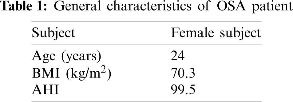
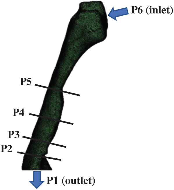
Figure 1: OSA patient (responder 1): The upper airway side view of the meshing airway model. The anatomical locations marked on the CT scan as P1, P2, P3, P4, P5 and P6 refer to: (P6) nasal choane level—inlet of the CFD model; (P5) minimum cross section area; (P4) tip of uvula; (P3 and P2) laryngopharynx; (P1) base of epiglottis—outlet of the CFD model

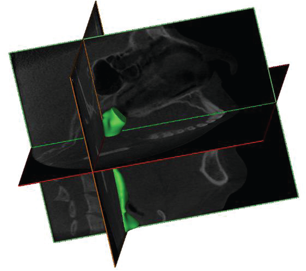
Figure 2: The airways of OSA patient 3D volume pharyngeal airway

The CT scan images were obtained while the patient was awake and positioned with the face lying upwards [13]. Each CT Scan had 534 pixels × 534 pixels and the pixel spacing was 0.3 mm × 0.3 mm. A series of CT scan images was saved in a Digital Imaging and Communications in Medicine (DICOM) format. After that, the DICOM images were imported into the 3D medical image processing software (Mimics, version 15.0; Materialise, Leuven, Belgium). Then, image segmentation was carried out to identify the 3D airway region based on the pixel information (Hounsfield units) from the DICOM image series. The airway model surface was generated by using the airway segment in the pulmonary function as clearly shown in Fig. 2. Based on the surfaces generated, the 3D volume of pharyngeal airway was built and then exported for the generation of the 3D model mesh.

3.2 Human Upper Airway Mesh Generation

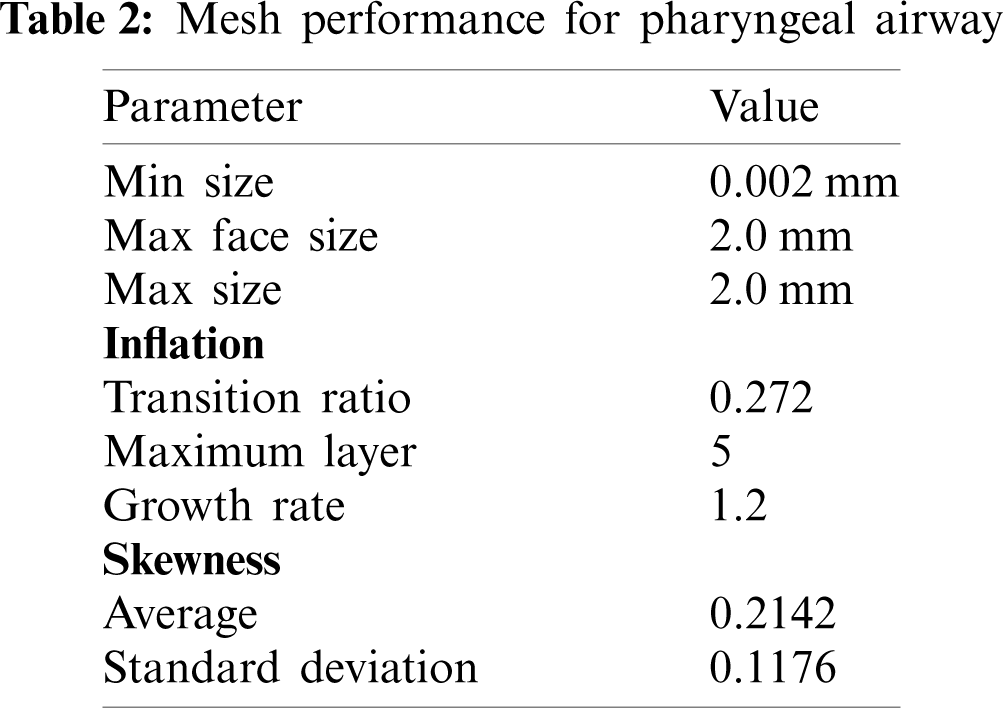
The 3D model generated by the Mimic software was transferred to 3Matic (version 15.0; Leuven, Belgium) to create the volume mesh. The pre-processor ICEM (ANSYS, USA) was used to generate the unstructured tetrahedral meshes for airway volumes as shown in Fig. 3. The quality of mesh was controlled to ensure the highest level of accuracy. The meshing parameters are summarized in Tab. 2. The surfaces of pharyngeal airway were meshed with 2.0 mm of max face size. The maximum and minimum sizes for the mesh were 2 mm and 0.002 mm, respectively. Inflation of the pharyngeal airway mesh around the wall boundary was considered in order to increase the accuracy of the simulation. Moreover, a sufficient fine mesh was created next to the wall, providing an adequate small mesh near the wall mesh size. The y+ (dimensionless distance) approach was used in estimating the initial boundary layer thickness [14] accurately, corresponding to the near-wall cell size (0.272). The quality of the airway meshed model was examined in ANSYS. The quality of mesh was measured by the average skewness value and the standard deviation. The value of skewness was 0.2142, which indicated that the cell quality was excellent (0–0.25) as recommended by ANSYS. Later, the mesh sensitivity grid study was performed on the 3D airway model alongside different grid scales. The 5-grid sizes were evaluated and found to have acceptable accuracies as shown by the previous research approach. This includes the meshing of the boundary layer as shown in Fig. 3.

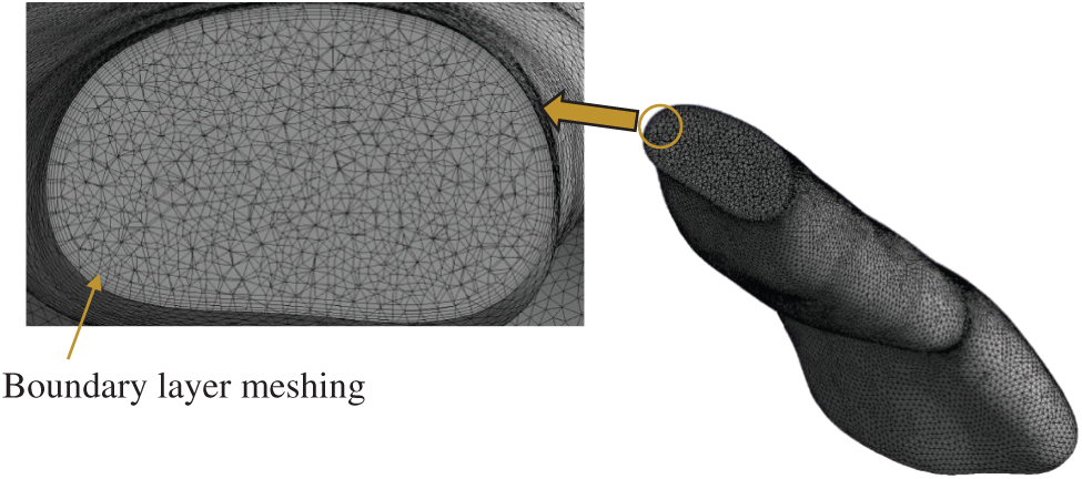
Figure 3: Cut-away view of computational grid system

3.3 Upper Airway Numerical Modeling

The airflow governing equations were discretized on the computational domain by using second-order finite-volume schemes. The coupling between the velocity and pressure fields was realized using the SIMPLE algorithm [15]. The boundary conditions consisted of axial velocity specification at the inlet plane to match the desired mass flow rate, no-slip boundary conditions for velocity at the airway wall, and a flux-conserving zero-gradient condition at the outlet surface of the computational domain. Breathing during inhalation involves the air flow passing through the pharyngeal airway. The airflow characteristics may vary due to the uniqueness of the pharyngeal airway. Thus, in the simulation analysis, the flow fields for the OSA patient in the pharyngeal airway were computed by using a steady-state Reynolds averaged Navier-Stoke (RANS) formulation with the k−ω shear stress transport (SST) turbulence model and low Reynolds number correction [16]. The popular SST k−ω turbulence model was considered in the current study compared to the k−ϵ model due to its greater accuracy in the viscous near-wall region treatment and consideration of the effects of adverse pressure gradient [17].

The most prevalent technique used to model respiratory flows is the CFD framework of the steady-state Reynolds Averaged Navier-Stokes (RANS) with corresponding turbulence closures [18–22]. RANS can provide reliable time-average data for a specific flow field with adequate tuning of the empirical constants [17]. It is robust and fast, but only in terms of quantities averaged over time, and the dynamics of the flow field cannot be predicted. However, it allows the airway models to be quickly screened to obtain useful average airflow and airway resistance data. The more complicated and time-intensive methods provide an increased level of detail and precision for unsteady, separated, or vortical turbulent flows [23].

3.4 Boundary Condition

The boundary conditions (i.e., inlet (P6), outlet (P1) and wall boundary) of the 3D model were defined via the surface of the model as mentioned in Section 2.0 (Fig. 1). The steady state turbulent airway flow was computed by ANSYS Fluent, which solved the finite volume using fitted grids. During the inhalation breathing, the velocity profile was assumed to be uniform and the axial component of the velocity was perpendicular to the flow inlet, nasopharynx [6]. A light breathing was considered at the inlet and 7.5 L/min of volume flow rate was used in the simulation [24]. 10% of the turbulent intensity was considered sufficient to mimic the real conditions and the outlet was defined by an average gauge pressure of 0 Pa [20,25]. In terms of heavy breathing, the turbulent intensity and outlet boundary conditions still remained. Heavy breathing was considered at the inlet and 30 L/min of volume flow rate was used in the simulation [6]. Opening boundary conditions, aimed at allowing flow entrainment through the boundary, were used for inlet boundary conditions specified by atmospheric pressure (Pinlet = Patmo: Gauge pressure is 0 Pa). Because the flow pressure change within the nasal cavity is relatively smaller (approximately 10%) than that within the pharyngeal airway, the atmospheric pressure was applied at the inlet boundary. With the assumption that pressure changes within the nasal cavity are negligible, the nasal cavity area was excluded in the simulation domain.

The method used to determine the detailed computational airway flow is described in this section. The method used in the current study included both CFD modeling and segmentation of CT-scan acquisition. For the CFD modeling, the model was considered on the segmentation of the pharynx in the human upper airway as seen in Fig. 1. The volume of the model was created based on the CT scan images. As the inhalation breathing was focused on the simulation, the marked locations P6 and P1 were defined as the inlet and outlet boundary conditions, respectively. In the simulation, the TKE of the upper airway was obtained by considering all important parameters and boundary conditions as used in previous researches.

3.5 Grid Sensitivity and Solver Verification

The grid sensitivity test was crucial for the CFD simulation to ensure that the generated grid could provide consistent and converging simulation results. In the current work, two different validation studies (i.e., grid sensitivity and solver verification) were carried out to demonstrate the adequacy or capability of the CFD formulations when analyzing the pharyngeal airway. The grid sensitivity test was used by Zheng et al. [26] with a total of five different elements to confirm the reliability of the predicted results for the analysis of the human upper airway. Thus, we adopted the similar practices and model that were used. Furthermore, a comparison was made between the current results and the previous simulations (RANS, k-omega, SST) as well as experimental results from Mihaescu et al. [27] and Mylavarapu et al. [20]. The grid sensitivity test has been used to determine and verify the optimum grid required to provide both consistent and accurate CFD results. As reported by Zheng et al. [26] and Zhao et al. [7], they used 1.3 million-elements to analyze the pharyngeal airways that resulted in an acceptable accuracy and further saved up to 30% of computational time compared to those with more elements.

In the current grid sensitivity test, the change in the wall static pressure on a selected plane was used as a convergence criterion. The wall static pressure dropped when the total of elements increased as shown in Fig. 4. Grid 5 and Grid 6 demonstrated the obvious convergence state with only a small difference (0.25%) in the wall static pressure. Taking into consideration the computational time and accuracy, Grid 5 (1.29 million-elements) was more practical for the simulation analysis. Therefore, Grid 5 was considered in the current simulation analysis as it met the criteria and was more practical to be used in the simulation. Furthermore, the Grid 5 airway model results were compared with the previous experimental and simulation results. The current simulation results showed a nearly identical trend compared to the previous works as shown in Fig. 5. Thus, the simulation model and solver (RANS k−ω SST) were reliable and validated for the study of the pharyngeal airway.

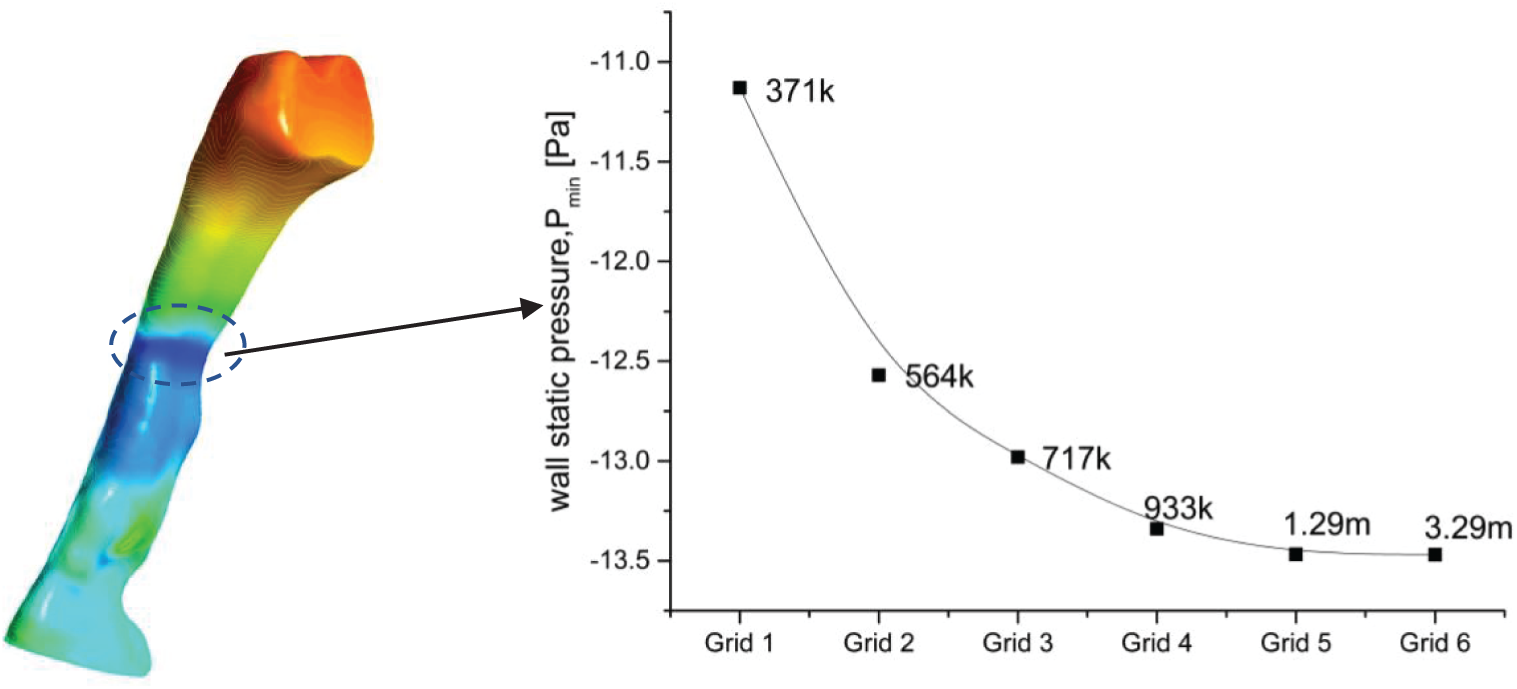
Figure 4: Focus point and grid sensitivity test of the upper airways OSA patient

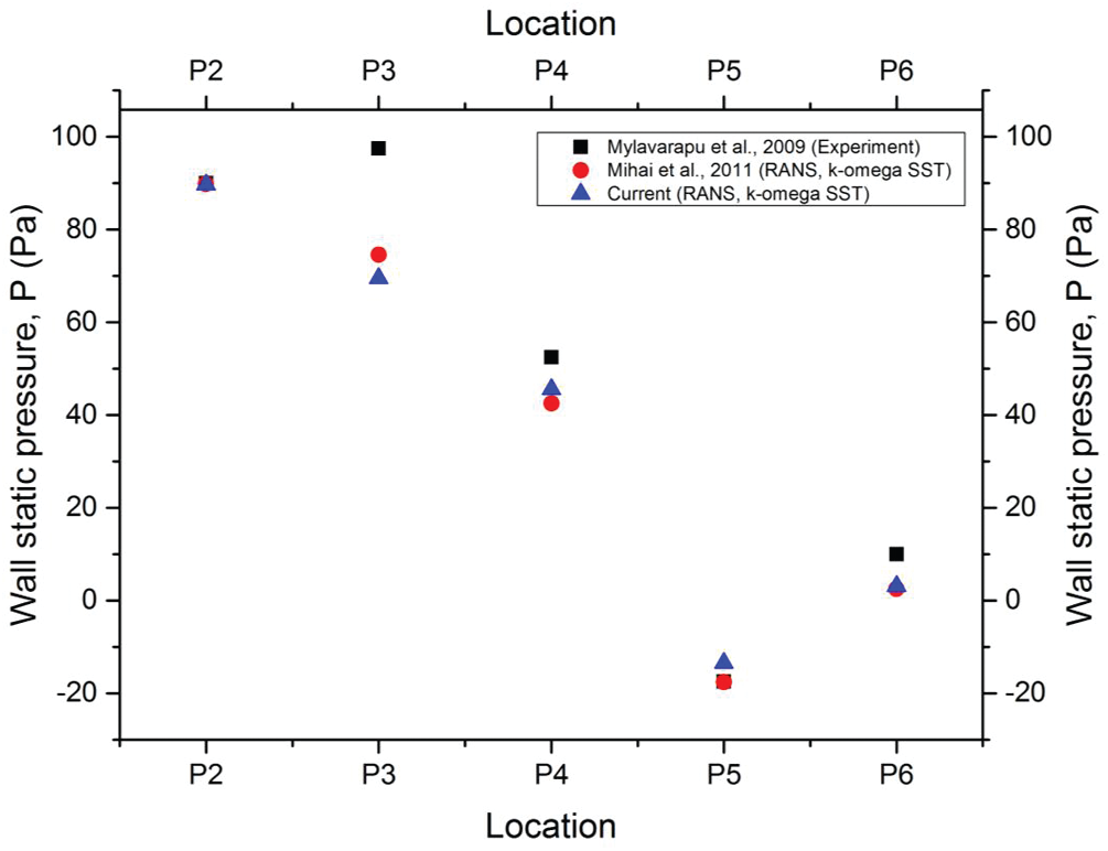
Figure 5: Comparison with previous experimental results

3.6 Limitations of the Study

Some of the limitations of this study include the limited extent of the airway under study, the fact that the velocity of breathing is considered uniform, patients were awake and in an upright posture during the scans, the absence of a sleep study, the lack of sleepiness scales or questionnaires, the unknown stage of respiration, and the lack of tongue control. In addition, the airway is not a rigid structure, and the effects of the soft tissue flaccidness could not be taken into consideration.

4  Results and Discussion

The CFD simulation results of airway analysis is significant and could be useful to the medical practitioner because these results provided a clear visualization of the airflow. The assessment of the current airway analysis was focused on various aspects, such as the cross-sectional area, airflow patterns, velocity, pressure, skin friction coefficient, turbulence kinetic energy and turbulent Reynolds number. The variation in areas demonstrated the real anatomy of the patient's upper airway. The cross-sectional plane was used to identify the minimum area of the upper airway, indicating that the patient had the minimum cross-sectional area of 7.68 mm2 at location 28 mm from the inlet.

In patients who have sleep apnea, the minimum cross-sectional area is crucial. The contraction of the cross-sectional area influences the smoothness of the airflow when passing through the upper airway. This situation also defines the obstruction of the airflow during the inhale breathing. The narrow area of the airway may be caused by the collapse or laxity of airway tissue. Thus, different OSA patients may have different airway features. As mentioned before, the RANS k -- ω SST formulation was applied to simulate the airflow of a patient who had OSA during the inspiration phase of normal breathing at 7.5 L per minute (L/min). The breathing rate used was similar to the one by Powell et al. [6] during their investigation of flow patterns in the pharyngeal airway. The flow values such as velocity, pressure and skin friction coefficient were popularly reported by most researchers such as Zhu et al. [28], Mortazavy Beni et al. [29] and Pirnar et al. [30] to describe and explain the airflow characteristics of the upper airway. In the current study, the additional flow parameter, turbulence kinetic energy (TKE), was considered to further describe the airflow characterization inside the upper airway. Other flow parameters were also considered in visualizing the phenomena and flow pattern in the upper airway.

4.1 Pressure and Skin Friction Coefficient

As air passes through the airway, the airway walls or tissues experience the variations in static pressure. Pressure variation may lead to the vibration of the airway tissue. Figs. 6a and 6b illustrate the static pressures on the airway wall (unit: Pa) and the distribution along the pharyngeal upper airway during the inspiration phase for both light breathing (normal) and heavy breathing. The pressure for both light and heavy conditions presented here were solely for the baseline case. The location of low pressure was almost the same location for both conditions (light and heavy breathing). The low pressure started to occur around the minimum cross-sectional area (7.68 mm2). This condition was described by the Bernoulli principle, while the rise in airflow velocity in the minimum area lowered the static pressure at the same time. It also decreased the airflow's potential capacity. The simulation results showed the highest pressure drop (–2101.3 Pa) around the minimum cross-sectional area during heavy breathing. Therefore, the low airway pressure phenomenon in this area would lead to higher velocities and maximum shear stress, eventually producing high turbulence and causing vibration [31].

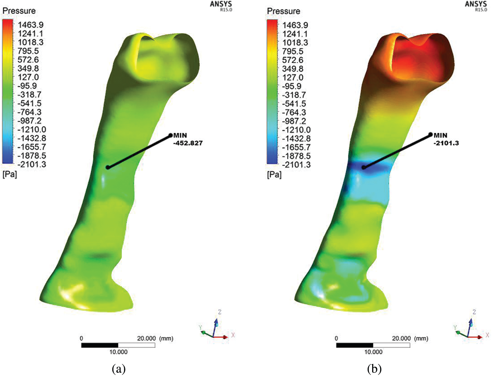
Figure 6: Comparison of pressure distribution at wall for light breathing (a) and heavy breathing (b) for the OSA patient

Figs. 7a and 7b present the skin friction coefficient distribution on the wall along the pharynx. The data presented here are only for the baseline case. The maximum and minimum wall skin friction coefficients were observed at the minimum cross-sectional area or obstructed regions. The skin friction coefficient corresponded to the pressure variation during the breathing. Therefore, the maximum skin friction coefficient was concentrated around the minimum cross-sectional area of the airway. The skin friction coefficient occurring would generate the boundary layer [32]. This would further cause turbulence and generate vibration or snoring during sleep [33]. The occurrence of vibration could cause worse impact that led to the relaxation of the pharyngeal tissue. Moreover, in this situation, the flow recirculation regions with negative axial velocities were easily formed in the downstream regions with the obstructions.

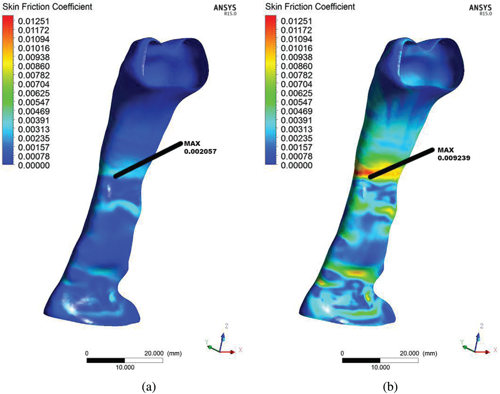
Figure 7: Comparison of skin friction coefficient derived from the flow in the upper airway for the OSA patient in light breathing (a) and heavy breathing (b)

4.2 Airflow Pattern in Pharyngeal

The airflow pattern was studied to understand its behavior when passing through the upper airway as characterized by different cross-sectional areas and shapes. As presented in Fig. 8, six planes (Planes 1–6) were considered to visualize the detailed computational analysis results in the upper airway of the OSA patient. The airflow pattern was described in detail via airflow parameters such as velocity, Reynold number and TKE. Therefore, it is important to present the results according to each plane in order to understand the behavior and mechanism of flow inside the pharynx. As illustrated in Fig. 8, the airflow direction started from the inlet and flowed to the outlet.

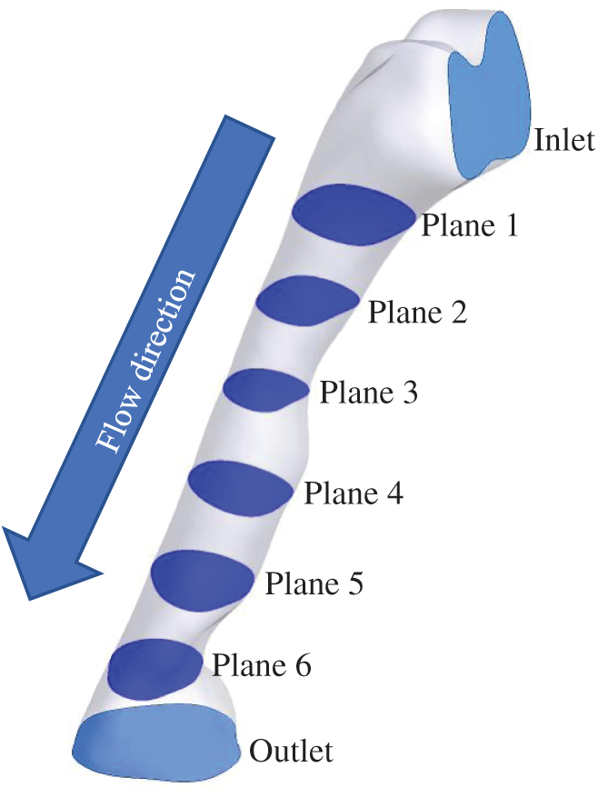
Figure 8: 6 planes used for airflow visualization

4.2.1 Velocity Profile

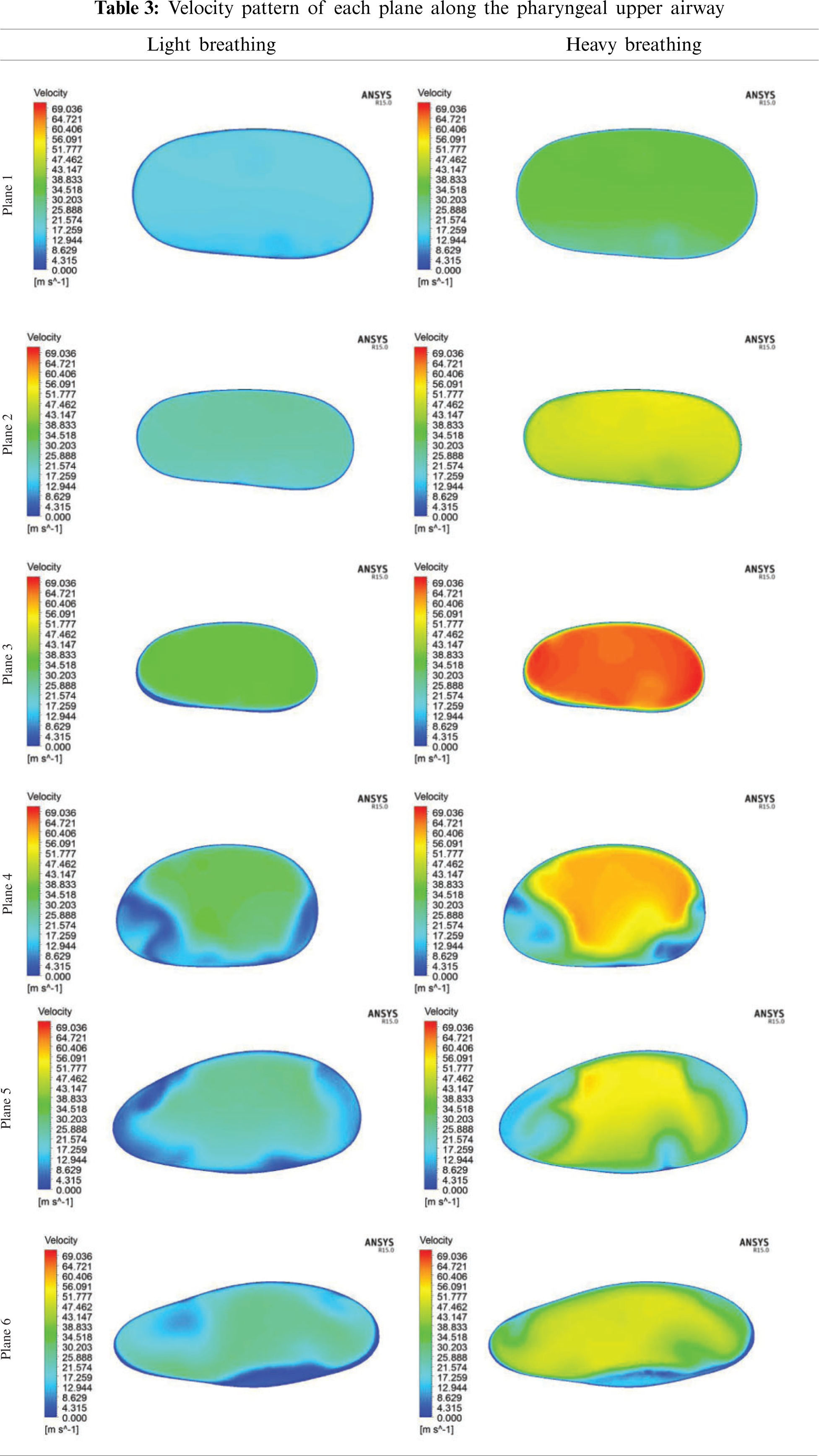
As aforementioned in Section 4.1, the pressure drop due to the obstructed region might lead to flow recirculation around the downstream region. Thus, the velocity profile was further investigated in the simulation of the upper airway. Tab. 3 shows the velocity profile in each plane along the pharynx and the velocity contours of Planes 1–6 are compared for both light and heavy breathing. In Fig. 9, both light and heavy breathing demonstrated the almost identical trend along the pharynx with different values of velocities. The simulation results noticed that the maximum velocity occurred at 0.03 m (occur at the minimum cross section area) from the inlet. This phenomenon was also observed by Singh et al. [34], whereas the velocity and turbulence intensity slightly elevated at the stenosis area. The velocity contour of both light and heavy breathing showed the highly similar pattern as shown in Plane 3 (Tab. 3). The highly uniform airflow was fully occupied in Planes 1–3 during both light and heavy breathing.

Interestingly, the disturbance of the velocity contour was observed during both light and heavy breathing after the airflow passed through Plane 3 (obstructed region). It meant that the particles in this region had the highest skin friction coefficient, as shown in Fig. 7. After position 3, the velocity started to decrease as shown in the graph. Similarly, the velocity contour in Plane 4 illustrated the uneven contour distribution. High velocities did not fully occupy Plane 4. This phenomenon was attributed to the expansion of the airway after the obstructed region (Plane 3). The sudden drop of velocity at Plane 5 during the heavy breathing might be attributed to the shape and expansion of cross-sectional area (at 0.05 m from inlet). The airflow velocity decreased when passing through Planes 5 and 6 until exiting the outlet. The flow condition of the airflow can be further explained by the Reynolds number.

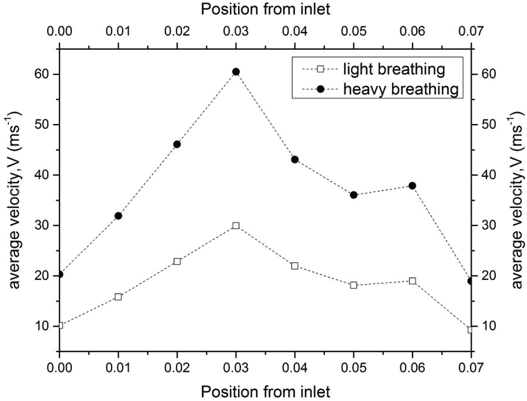
Figure 9: Velocity distribution along the pharynx for light and heavy breathing

4.2.2 Reynolds Number

In the current study, the Reynold number was used to explain the flow conditions, either in laminar or turbulent flows. The Reynold number is often used to express the intensity of turbulence or flow condition in airway studies by previous researchers. Fig. 10 presents the Reynold number in the pharynx. The Reynold number plots showed a nearly similar trend with the velocity profile as discussed in the section above because the Reynolds number corresponded to the changes in the velocity profile. For the internal flow, a Reynolds number of more than 4000 is considered to be a turbulent condition. For light breathing, the position 0.03 m from the inlet experienced turbulent phenomena (Re>4000). However, the flow in the transition phase from the inlet until it reached position 0.03 m. The flow was diverted to transition again after passing Plane 3. Inversely, for the heavy breathing, the flow along the pharynx was always in turbulent condition (Re = 80000).

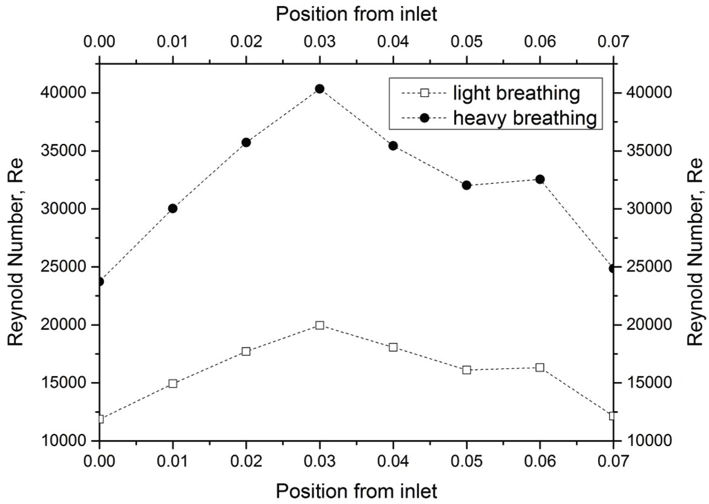
Figure 10: Reynold number of light and heavy breathing

4.2.3 Turbulent Reynolds Number

The turbulent Reynold number was considered in the current study to explain the energy of the Reynold number as expressed in Eq. (6). The turbulent Reynold number reflects a level of turbulence within a given area (Planes 1–6) of the airway. Fig. 11 depicts the turbulent Reynolds number for both light and heavy breathing. A high turbulent Reynolds number indicates that the air flowed with high kinetic energy and less work of friction in the human airway. The results revealed the kinetic energy of airflow increased suddenly after the air flowed through the obstructed region (minimum cross-sectional area, Plane 3). Therefore, the airflow profile was unevenly distributed in Planes 4–6 as observed in Tab. 3 (Section 4.2.1).

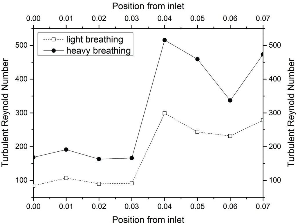
Figure 11: Turbulent Reynold Number based on Eq. (6)

Tab. 4 shows a comparison of the turbulent Reynolds number for light and heavy breathing. The maximum turbulent Reynold number was at position 0.04 m (Plane 4) when the airflow passed through the Plane 3. This expansion after Plane 3 increased the kinetic energy of airflow particle, causing the vortex formation in this region. This phenomenon was observed in Planes 4 and 5 (Tab. 4). However, the turbulent Reynolds Number occurring at Planes 4, 5 and 6 only gives a limited understanding of the flow mechanism. The concentration and strength of the turbulence are not reflected in the turbulent Reynold number, but can be seen in Turbulent Kinetic Energy.

4.3 Turbulent Kinetic Energy (TKE) in Pharynx

In the current study, the TKE was considered to describe the airflow characteristics in the airway for the OSA patient. TKE describes the turbulent fluctuations of the airflow. The occurrence of turbulent fluctuation may lead to unintended tissue vibration. Furthermore, severe vibration of the airway tissue leads to snoring. Long-term snoring weakens the airway tissue and hence causes the blockage of airflow leading to sleep hypopnea and apnea. The TKE is associated with the kinetic energy of vortexes (velocity fluctuation) generated in the turbulent flow, quantifying the turbulence level in the airway. However, the turbulent Reynold number reflects a level of turbulence in a given area, i.e., a cross-sectional area of the airway.

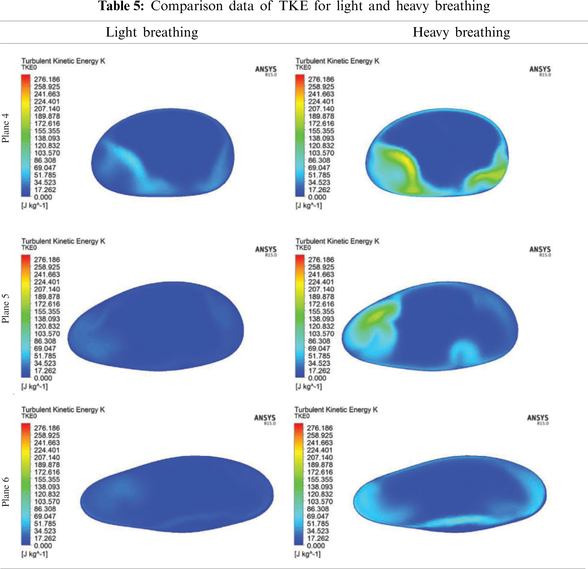
In the CFD analysis, the TKE and turbulent Reynold number, Rey were computed. The distribution of TKE along the airway is shown in Fig. 12 and the contour of TKE is depicted in Tab. 4. The TKE were obtained from the fluctuation velocity as shown in Eq. (4). Accordingly, the turbulent Reynold number was computed from Eq. (6) as explained by Vladimir et al. [11] and Katragadda et al. [35]. The airflow motion in the airway is predominantly caused by the energy in turbulent flow and anisotropy effects. Therefore, the TKE is suitable to describe the vortex and quantify the turbulence level. The results show that high TKE is concentrated around the region following the narrow region due to the expansion of the airway after the obstructed region as discussed in the previous section. Besides that, the jet formation was observed in the pharynx of the airway. The jet formation phenomenon hit the wall in the inhale breathing, causing velocity remodeling near the airway wall. The TKE that occurred for the high fluctuation velocity induced from the recirculation phenomena is shown in Tab. 5. The recirculation phenomena might generate vibrations on the surrounding airway tissue, thus leading to snoring. Therefore, the TKE value is useful to provide new information on the airflow characteristics, and as a new parameter to characterize as well as detect patients with OSA.

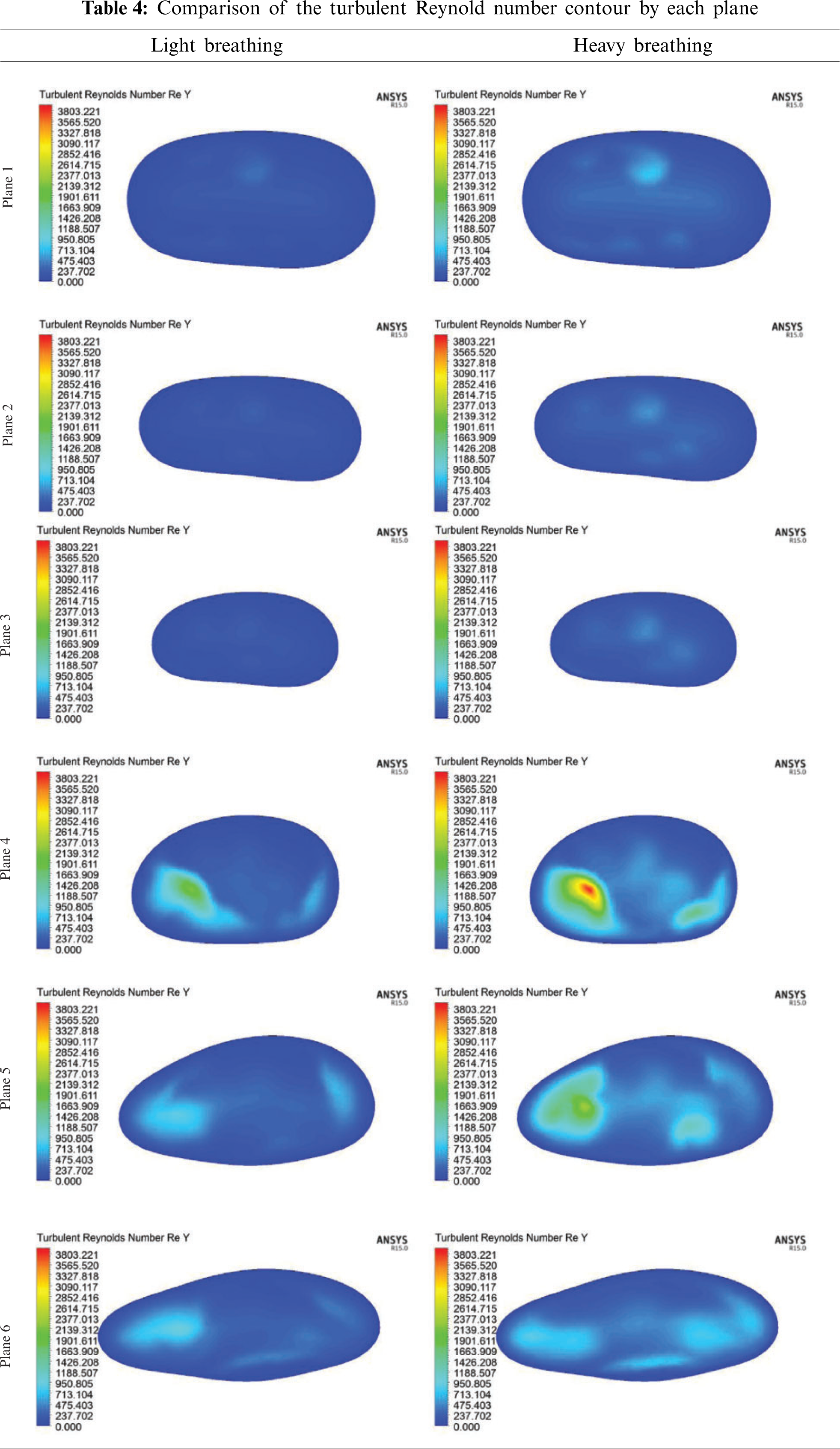
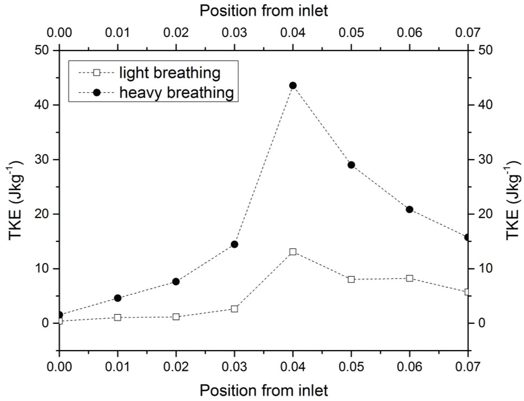
Figure 12: TKE of the upper airway along the pharynx for both light and heavy breathing

5  Conclusion

In this study, the feasibility of using computational analysis to analyze airflow characteristics has been investigated. Based on the results of this investigation, the following conclusions can be made.

•   The airflow characteristics were explained by parameters such as pressure distribution, skin friction coefficient, velocity profile, Reynolds number, turbulent Reynolds number and turbulence kinetic energy. CT scan data was used to create the 3D model of the patient's airway using Mimic software and the simulation was carried out using ANSYS FLUENT. The 3D model and solver were validated through the grid sensitivity test as well as experimental results from previous studies.

•   The solution of the turbulent kinetic energy equation can be used to construct energy balance, and detailed relationships between the convection, diffusion, production and dissipation of turbulent kinetic energy can be obtained.

•   The comparison of light and heavy breathing indicated that the presence of the turbulent flow might lead to the vibration of airway tissue and weakening of the tissue's strength, thus inducing snoring and causing the OSA. The current results are useful to provide a clear visualization to understand the airflow characteristics under light and heavy breathing for the medical practitioners in the OSA research area.

•   The use of this computational method to construct turbulence kinetic energy balance is an effective technique for evaluating the severity of obstructive sleep apnea.

Funding Statement: This work is supported by the Fundamental Research Grant Scheme provided by the Ministry of Higher Education (Ref. No. FRGS/1/2020/TK0/UNIMAP/03/26) and University of Malaya Grant (Ref. No. GPF020A-2019). The authors extend their appreciation to the Deanship of Scientific Research at King Khalid University for funding this work through the General Research Project GRP/281/42.

Conflicts of Interest: The authors declare that they have no conflicts of interest to report regarding the present study.

This work is licensed under a Creative Commons Attribution 4.0 International License, which permits unrestricted use, distribution, and reproduction in any medium, provided the original work is properly cited.