Computer Modeling in Engineering & Sciences

DOI: 10.32604/cmes.2021.014239

ARTICLE

High Order of Accuracy for Poisson Equation Obtained by Grouping of Repeated Richardson Extrapolation with Fourth Order Schemes

Luciano Pereira da Silva1,*, Bruno Benato Rutyna1, Aline Roberta Santos Righi2 and Marcio Augusto Villela Pinto3

1Graduate Program in Numerical Methods in Engineering, Federal University of Paraná, Curitiba, 81531-980, Brazil
2Graduate Program in Space Sciences and Technologies, Aeronautics Institute of Technology, São José dos Campos, 12228-900, Brazil
3Department of Mechanical Engineering, Federal University of Paraná, Curitiba, 81531-980, Brazil
*Corresponding Author: Luciano Pereira da Silva. Email: luciano.silva@ufpr.br
Received: 12 September 2020; Accepted: 12 March 2021

1  Introduction

One of the main goals of researchers is to obtain improved numerical methods capable of solving problems that hinder technological progress, as well as those related to Engineering. In particular, one of these problems is characterized by the determination of the numerical solution of the Navier-Stokes (NS) equations, which require a large computational effort when determining the numerical solution of the continuity equation, represented by the Poisson equation. The simplified two-dimensional Poisson equation is given by

∂2u∂x2+∂2u∂y2=-f,inΩ,(1)

along with boundary conditions relating to the Ω domain of the problem. Some studies, including Poisson equation, present solutions using compact fourth and sixth order methods with direct methods to solve the system of equations [1]. In addition, they have found results including higher order of accuracy on non-uniform grids to determine critical grids that violate [2] stability conditions. In [3] the Eq. (1) was solved numerically by combining the standard multigrid method and Repeated Richardson Extrapolations (RRE), where solutions of sixth order of accuracy were obtained. In the work of [4] an unconventional compact nine points form was introduced, named as Exponential Difference Scheme based on the Finite Difference Method (FDM).

This work includes higher order methods for discretizing Eq. (1) based on FDM [5]. These methods belong to a group of higher order schemes, where the combination of FDM approximations results in new methods that consider a larger number of neighboring points. They are: the Compact Finite Difference Scheme of fourth order (Compact −4) [3]; and the Exponential Finite Difference Scheme of fourth order (Exponential −4) [4]. In addition, the higher order methods in conjunction with the standard multigrid Full Approximation Scheme (FAS) [6] provide faster convergence to the numerical solution. One can also determine significantly better results when applying a fourth order of accuracy scheme with nine points, due to the decreased discretization error. To determine numerical solutions with higher order of accuracy, the post-processing method known as RRE can be used [7–9].

The main goal of this work is to obtain successive accurate solutions for Eq. (1) in an efficient way without increasing the computational time. For this, we use RRE that combines nine numerical solutions using quadruple precision (Real * 16 or extended precision) in order to obtain tenth order precision solutions. The grids have a refinement ratio q = 2 from 9×9 to 2049×2049. The numerical solutions included in the present work were obtained using FORTRAN language.

This work is subdivided as follows: In Section 2 we present the proposed mathematical and numerical model; In Section 3 the applied fourth order methods; In Section 4 we describe the RRE method used to obtain the tenth order of accuracy of the numerical solution; In Section 5 we show the standard multigrid method; In Section 6 the numerical tests and results, and, in Section 7 the conclusions of the work.

2  Mathematical and Numerical Models

The main goal is to solve the two-dimensional Poisson equation, represented by (1), and to achieve tenth order of accuracy numerical solutions. For this, the first step is to find the best fourth order scheme applying the standad FAS, and from that apply the RRE. Therefore, there is no problem in taking a simple domain with a discretization in simple grids, because the standard multigrid could be applied in non-orthogonal grids or unstructured grids [7]. As the RRE is a post-processing [10], its application is independent of how data were collected.

This section describes the model of the equation, its domain, boundary conditions and analytical solution that will be used by means of comparison and verification.

Given the equation

∂2u∂x2+∂2u∂y2=-f,inΩ=(0,1)×(0,1),(2)

with boundary conditions obtained by the analytical solution, the unit square domain was discretized applying uniform grids with h: = 1/(Nx −1) and k: = 1/(Ny −1), for x and y directions, respectively. Here, Nx and Ny represent the number of grid points in coordinate directions x and y, respectively. Therefore, these grid points are defined by (xi,yj), where xi: = ih and yj: = jk, for 0≤i≤Nx-1 and 0≤j≤Ny-1.

Considering an uniform grid by direction with elements size h and k for each of the coordinate directions x and y, respectively. The approximations for the partial derivarives are given by Central Difference Scheme of second order (CDS −2) [5].

∂2u∂x2|i,j=Ui-1,j-2Ui,j+Ui+1,jh2-h212∂4u∂x4|i,j-h4360∂6u∂x6|i,j+O(h6)(3)

and

∂2u∂y2|i,j=Ui,j-1-2Ui,j+Ui,j+1k2-k212∂4u∂y4|i,j-k4360∂6u∂y6|i,j+O(k6).(4)

Replacing Eqs. (3) and (4) in Eq. (1) the equation is obtained from which the estimate Eq. (5) is derived

Ui-1,j-2Ui,j+Ui+1,jh2+Ui,j-1-2Ui,j+Ui,j+1k2=-fi,j.(5)

The approximations given by Eqs. (3) and (4) result in the asymptotic order pL = 2 and true orders pm=2,4,6,… in Eq. (5) [11]. We describe how to increase the order of this discretization method for two known high order methods in the next section.

3  High Order Methods for Poisson Equation

3.1 Compact Finite Difference Scheme

Given Eq. (1), where U is the solution of Eq. (5) through a second order approximation. Therefore, in order to determine approximations for fourth order derivatives and obtain the known compact fourth order method, it is necessary to expand the following terms:

∂4u∂x4|i,j=-∂2f∂x2|i,j-∂4u∂x2∂y2|i,j,(6)

and

∂4u∂y4|i,j=-∂2f∂y2|i,j-∂4u∂x2∂y2|i,j.(7)

Then, replacing Eqs. (6) and (7) in Eqs. (3) and (4), respectively. Furthermore, considering a CDS −2 approximation for the second order partial derivative of f(x,y), we have

∂2u∂x2|i,j=Ui-1,j-2Ui,j+Ui+1,jh2+112(fi-1,j-2fi,j+fi+1,j)+h212∂4u∂x2∂y2|i,j-h4144∂4u∂x4|i,j+O(h4),(8)

and

∂2u∂y2|i,j=Ui,j-1-2Ui,j+Ui,j+1k2+112(fi,j-1-2fi,j+fi,j+1)+k212∂4u∂x2∂y2|i,j-k4144∂4u∂y4|i,j+O(k4).(9)

For ∂4u/(∂x2∂y2)|i,j, the approximation is

∂4u∂x2∂y2|i,j=4Ui,jh2k2-2(Ui-1,j+Ui+1,j+Ui,j-1+Ui,j-1h2k2)+Ui-1,j-1+Ui-1,j+1+Ui+1,j-1+Ui+1,j+1h2k2+O(h2,k2).(10)

Next, Eq. (10) is replaced in Eqs. (8) and (9). After that, summing up both resulting equations leads to

Ui-1,j-2Ui,j+Ui+1,jh2+Ui,j-1-2Ui,j+Ui,j+1k2+(h2+k212)[4Ui,jh2k2-2(Ui-1,j+Ui+1,j+Ui,j-1+Ui,j+1h2k2)+Ui-1,j-1+Ui-1,j+1+Ui+1,j-1+Ui+1,j+1h2k2]=112(fi-1,j+fi+1,j-8fi,j+fi,j-1+fi,j+1).(11)

Later, considering k = h and rearranging Eq. (11), we have

Ui,j=310[Fi,j+23(Ui+1,j+Ui-1,j+Ui,j-1+Ui,j+1)+16(Ui+1,j+1+Ui-1,j+1+Ui+1,j-1+Ui-1,j-1)]h2,(12)

where

Fi,j:=112(fi-1,j+fi+1,j-8fi,j+fi,j-1+fi,j+1).(13)

According to [12], the local truncation error is given by

τi,j=-h4360(∂6u∂x6+∂6u∂y6)(i,j)+O(h6).(14)

Finally, by Eq. (14) it is possible to stablish the asymptotic, pL = 4, and true orders, pm=4,6,8,…, respectively.

After some algebraic manipulations, the stencil model is

103h2[000010000]h-23h2[010101010]h-16h2[101000101]h=112[0101-81010]h.(15)

Therefore, Eq. (15) is the stencil of the approximation by Compact −4 for the two-dimensional Poisson equation in an unit square domain applying uniform grid elements based on approximations of [3,13,14].

3.2 Exponential Finite Difference Scheme

According to [4,15,16], the approximation Exponential −4 is accomplished from the following formulation:

∂2u∂x2+∂2u∂y2=f(x,y)eϕ(h).(16)

Then, assuming that k = h, by substituting the approximations from Eq. (11) on the left of the equality in Eq. (16), we get

ao(Ui-1,j+Ui+1,j+Ui,j-1+Ui,j+1h2)+a1(Ui-1,j-1+Ui-1,j+1+Ui+1,j-1+Ui+1,j+1h2)+a2Ui,j=b0fi,jeϕ(h),(17)

where

ϕ(h)=h2∇2fi,j12fi,j.(18)

Furthermore, the laplacian of Eq. (18) can be approximated, according to [5], by CDS −2. Thus, it results in

h2∇2fi,j=fi-1,j+fi+1,j-4fi,j+fi,j-1+fi,j+1,(19)

then,

ϕ(h)=fi-1,j+fi+1,j-4fi,j+fi,j-1+fi,j+112fi,j.(20)

According to [4], the constants are a0 = 4, a1 = 1, a2 = −20 and b0 = 6. Therefore, Eq. (17) can be rewrite as

4(Ui-1,j+Ui+1,j-4Ui,j+Ui,j-1+Ui,j+1h2)+(Ui-1,j-1+Ui-1,j+1+Ui+1,j-1+Ui+1,j+1h2)-20Ui,j=6fi,jeϕ(h).(21)

The local truncation error is given by [4] as

τi,j=h6240[4(∂6u∂x6+5∂6u∂x4y2+5∂6u∂x2y4+∂6u∂y6)-5(∂2u∂x2+∂2u∂y2)-1(∂4u∂x4+2∂4u∂x2y2+∂4u∂y4)2](i,j)+O(h8).(22)

Consequently, also according to [4], combining Eqs. (21) and (22) specifies the asymptotic, pL = 4, and true orders, pm=4,6,8,…, respectively.

The stencil of the approximation for the Poisson equation is given by

20h2[000010000]h-4h2[010101010]h-1h2[101000101]h=-6eϕ(h)[000010000]h,(23)

where

eϕ(h)=exp(112[0101-41010]h/[000010000]h).(24)

Therefore, Eqs. (23) and (24) stablish the approximation for Exponential −4 for the two-dimensional Poisson equation with uniform grid elements based on the approximations of [4].

Both for Eqs. (12) and (13) of Compact Scheme (with stencil given by Eqs. (15) and (21) of Exponential Scheme (with stencils given by Eqs. (23) and (24)), a system of the type AU=f is generated. This is a linear system with a sparse and large matrix, where iterative methods are the most suitable [5].

In the present work, we chose the nine points Gauss-Seidel solver (method for solving the linear system) in a lexicographic order for both discretizations in order to generate numerical solutions of such linear equations systems, whose matrices of coefficients are 9-diagonal diagonal given by algebraic manipulation of Eqs. (12) and (13) for Compact Scheme and algebraic manipulation of Eq. (21) for Exponential Scheme.

This Gauss-Seidel will be used as a smoother in the geometric multigrid method to determine the numerical solutions of the linear systems (see Section 4).

4  Repeated Richardson Extrapolation

For numerical analysis, Richardson Extrapolation (RE) [5] is an efficient technique of accelerating terms of a sequence that can be applied to reduce the discretization error of nodal numerical solutions. According to the Eq. (25), when combining two nodal solutions whith a refinement ratio q and order of accuracy p of the numerical method it is possible to determine ϕ∞, which is an estimate for the analytical solution.

Then, we have the equation

ϕ∞=ϕ2+ϕ2-ϕ1qp-1+E(ϕ∞),(25)

where ϕ2 and ϕ1 are solutions at the fine and coarse grid, respectively.

By applying RE repeatedly, we obtain the technique known as Repeated Richardson Extrapolation (RRE) [7,8,10,17]. The RRE is a post-processing technique used to decrease the discretization error of numerical solutions without increasing the number of terms in the finite difference equation obtained by the Taylor series, it depends only on the collected data. The RRE combines different grid solutions and for each extrapolation, the obtained solution presents a much smaller discretization error. This magnitude obeys the true orders in the finite difference equation used to approximate the derivatives of the differential equation. For this case, models of centered fourth orders were used based on CDS −2 approximations, thus, the true orders are pm={4,6,8,…} [17,18]. The expression for RRE is given by

ϕg,m=ϕg,m-1+ϕg,m-1-ϕg-1,m-1qpm-1-1,(26)

where ϕ is the numerical solution for the variable of interest (see Section 6), g is the grid where the numerical solution was obtained, m is the number of Repeated Richardson Extrapolations, pm are the true orders for the equation of the discretization error and q = hg −1/hg is the refinement ratio. In this work we use q = 2.

It is possible to approximate the asymptotic order of accuracy of each numerical method by the effective and apparent orders [11], respectively. The basis for the approximation is the numerical error (difference between analytical and numerical solutions) or by estimating the error of the numerical solution. The effective order (based on the numerical error) is given by [18].

pE=log(|Φ-ϕhg-1||Φ-ϕhg|)log(q),(27)

where Φ is the analytical solution and ϕ is the numerical solution of the variable of interest. In addition, hg −1 and hg represent the course and fine grids, respectively.

The apparent order (based on its estimation of the numerical solution error) is represented by [18]

pU=log(|ϕhg-1-ϕhg-2||ϕhg-ϕhg-1|)log(q),(28)

where q is the refinement ratio, ϕ is the numerical solution of the variable of interest and hg −2, hg −1 and hg represents the coarse grid, intermediate and fine, respectively.

To execute the RRE, pm = pE or pm = pU can be used in Eq. (26), which are the orders of accuracy of the numerical scheme, calculated according to Eqs. (27) and (28), respectively. The accuracy orders pE and pU are equivalent for the RRE. However, in order to use pE, the analytical solution must be known. In addition, to calculate pU, three nodal solutions are needed, while to calculate pE only two nodal solutions are sufficient. To show how the RRE is calculated, pm = pU is chosen, because in this case it is not necessary to know the analytical solution of the differential equation, and this makes the technique more robust.

The Algorithm 1 describes the steps to implement the RRE using pU, but can be easily adapted to use pE. In Fig. 1, the representation of one nodal numerical solution for the same point is shown in different grids and levels of extrapolation, where ϕg=G=9,m=4 is the solution of high order of accuracy associated with the g = 9 grid (note that there are only nine grids in the representation, so g = G = 9) after four Richardson extrapolations (m = 4) that are featured in the Fig. 1. It is important to note that at level m = 0 there is no extrapolation in the numerical solutions. The solution ϕ9,4 represents the output of Algorithm 1 for ϕ1…9,0, G = 9 and q = 2 as input data.

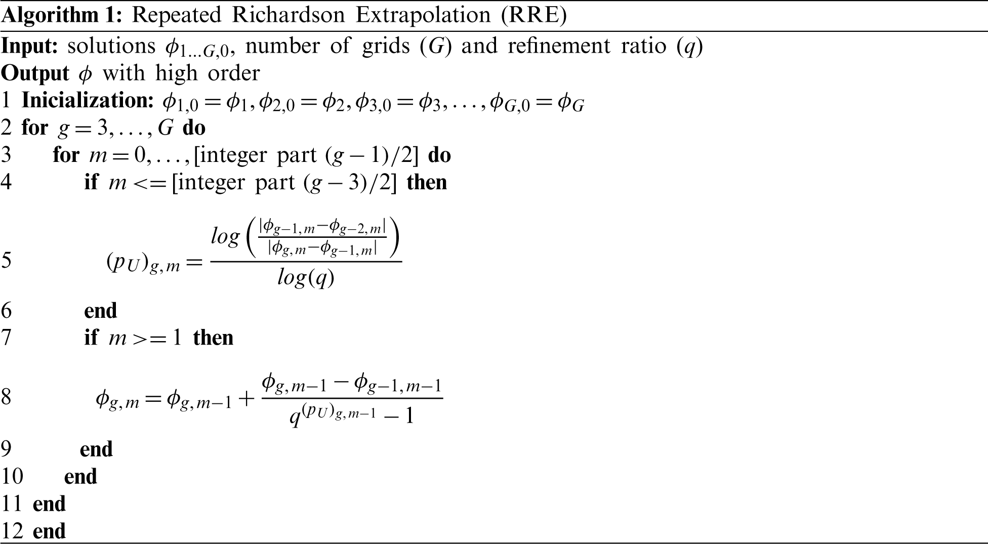
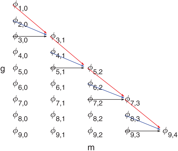
Figure 1: Schematic representation of RRE for g = 9 and m = 4

5  Multigrid Method (MG)

In general, the decrease in the discretization error is associated with the grid size, in other words, as much as the grid is refined, lower is the discretization error. However, highly refined grids result in large scale linear equation systems, which requires very high computational effort to achieve a numerical solution. Given that, in order to minimize the computational time used with highly refined grids, we adopted the multigrid method, which accelerates the convergence of standard methods using coarser grids as a support base.

Some classical iterative methods can reduce very quickly oscillatory modes errors of the finest grid leaving only smooth modes, where the method loses the effectiveness. Later, one should transfer information to the coarser grids (using restriction operators), where the smooth modes become more oscillatory, and then, the method becomes more effective. When reaching the possible or desired coarser grid, one should return with the information to the original finest grid of the problem (using prolongation operators). It speeds up the convergence of the method [6,19,20].

Depending on the type of information that is transferred between grids, one can use the Correction Scheme (CS) where only the residual is transferred, or the Full Approximation Scheme (FAS), where both residual and solution are transferred. In the present work, we chose the FAS method [6,19]. A cycle is the way that different grids are traversed. There are different types of cycles, for example, V-, W-, F-cycle [21,22] and we choose to appply the V-cycle because its lower computational coast [6,19]. The V-cycle is defined as V(ν1,ν2), where ν1 and ν2 are the numbers of pre and post-smoothing the multigrid cycle, in other words, the number of smoothing in restriction and prolongation process, respectively. Coarsening ratio (re) is the ratio of the distance between the consecutive points of the grid from de fine grid (h) and the coarse grid (H). In this work, we use re = 2, i.e., H = 2h [6,19].

In the present work, we adopt the standard geometric multigrid [23,24], that is usually recommended to orthogonal structured and non-orthogonal structured grids. However, for unstructured grids, the algebric multigrid can be applied [7,25,26].

The process of restriction (transfer information from the fine grid to the coarser grid) is carried out by the full weighting operator, defined by [6,19]

Ih2hvh(x,y)=116[121242121]h2h.(29)

The process of prolongation (transfer information from the coarse grid to the finer grid) is carried out by the bilinear interpolation operator, defined by [6,19]

I2hhvh(x,y)=12]010101010[2hh.(30)

6  Numerical Results

Approximations of AU=f were calculated in FORTRAN using quadruple precision, where AN×N is the matrix of coefficients, UN×1 is the vector of variables whose solution represents the temperature and fN×1=f(xi,yj)=fi,j is the source term in lexicographic order, given by f(x,y)=-cos(x+y)+cos(x-y). The boundary conditions obtained by the analytical solution u(x,y)=cos(x)cos(y). In addition, Rit=f-AUit is the defect of every each iteration (it).

The variables of interests are: the infinity norm (l∞) of the error based on the temperature Ui,j, the apparent and effective orders of the error based on the temperature at the midpoint, U(1/2,1/2), also, its defect |R(1/2)|. By that, one can analyze the decreasing in the module of the defect in the central point (|R(1/2)|) vs. the number of V-cycles (V(2,1)) by its dimensionless form represented by |Rit|/|R0|. To assure that the numerical solution admit only discretization errors, the absolute value of rit≈1×10-32 was calculated until it achieves its machine round-off error for the grids N=9×9,17×17,33×33,…,4097×4097. The numerical solutions for problems are obtained using computational programs written by the authors in Fortran 95 and using the Microsoft® Visual Studio® 2008 compiler v. 9.0.21022.8 RTM with quadruple precision and are run on a computer with a 3.40 GHz Intel® CoreTM i7-6700 processor with 16 GB of RAM hosting 64-bit Windows® 10.

The multigrid method FAS uses V-cycles, V(ν1,ν2) = V(2,1) with the maximum possible value of levels of grids. Operator of restrictions and prolongations are defined by Eqs. (29) and (30).

Our main contribution is, first, to find the best fourth order method, and then, combine it with the RRE. In this case, using the multigrid method in order to solve the problem in refined grids. Therefore, the CDS −2 is used only for purpose of comparison and verification of the computational code.

6.1 Verification of Truncation Error

Considering all the grids studied in this work, for keeping the same standard, we chose grids with N=2049×2049 e N=4097×4097 to represent all the ones adopted. It is possible to observe in Fig. 2 (for N=2049×2049 e N=4097×4097) that iteration errors for the CDS −2, Compact −4 e Exponential −4 methods decrease approximately one order of magnitude for every V(2,1)-cycle. Moreover, for both fourth order methods, the numbers of cycles were lower than 30 to reach the round-off error, while the second order method needed a slightly more than 35 V(2,1)-cycles.

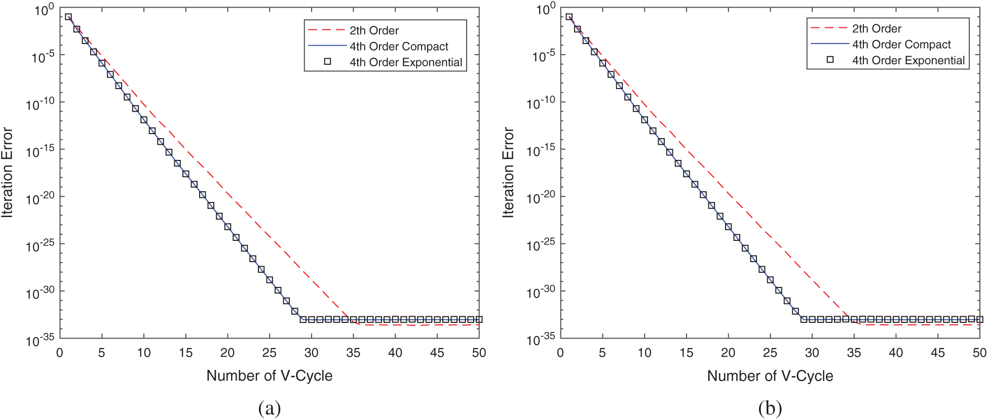
Figure 2: Iteration error vs. number of V-cycle for (a) 2049×2049 and (b) 4097×4097

Fig. 3 represents the effective order of the infinity norm (l∞) based on the error of the variable U(xi,yj). The Fig. 4 represents the effective order of the numerical solution error at the midpoint and Fig. 5 represents the apparent order of the numerical solution error at the midpoint.

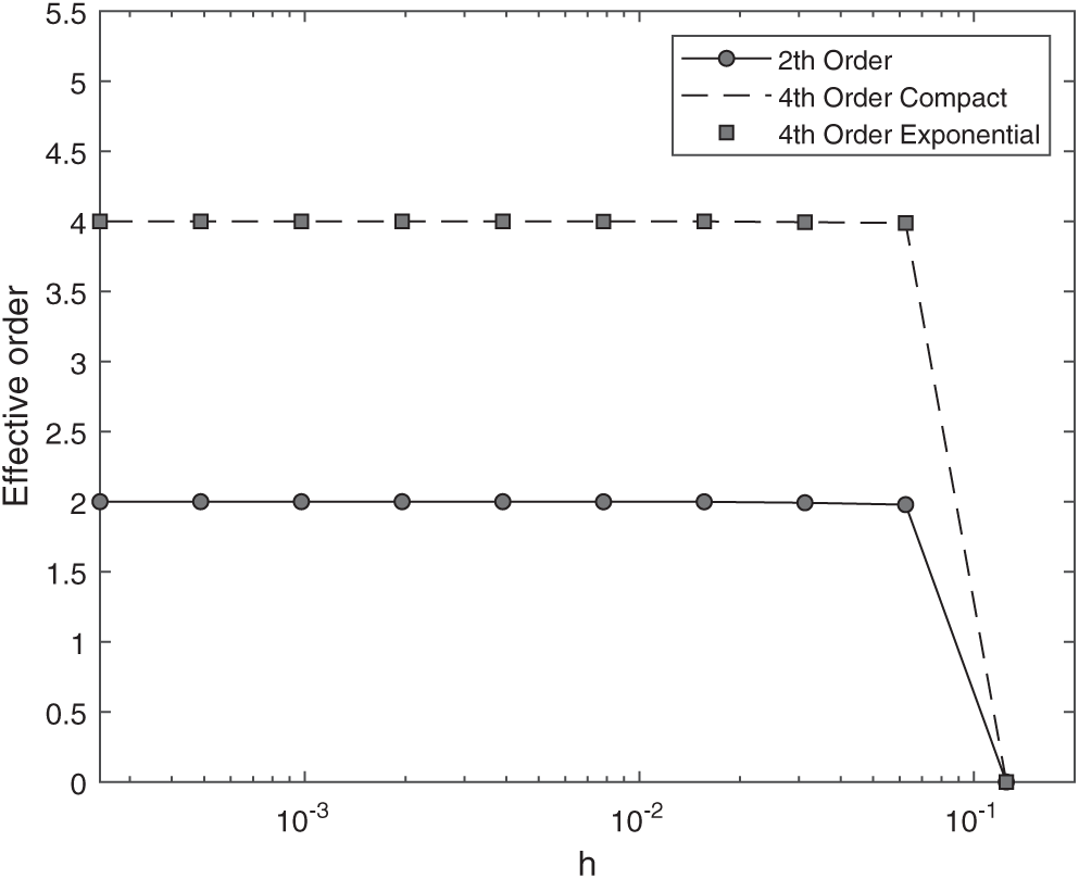
Figure 3: Effective order pE of accuracy based on l∞ of error

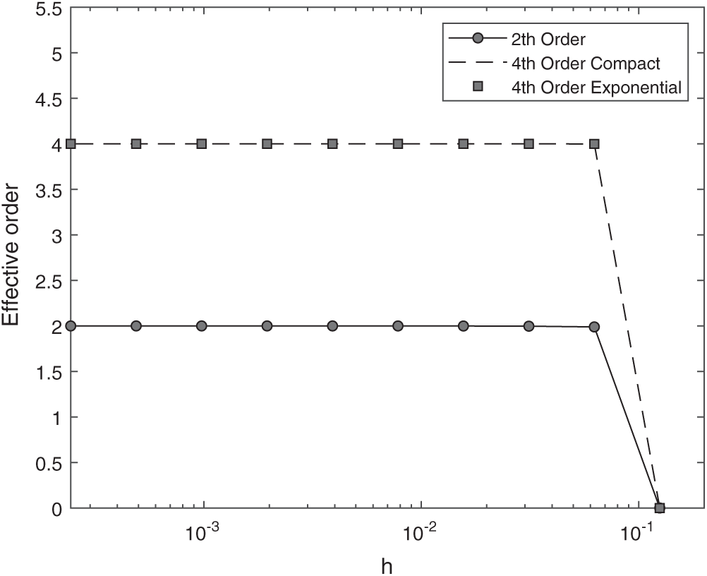
Figure 4: Effective order pE of accuracy in approximating U(1/2,1/2)

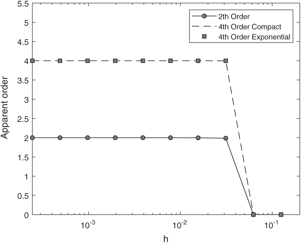
Figure 5: Apparent order pU of accuracy in approximating U(1/2,1/2)

One can observe in these figures that even for pE as for pU, also for any other variable of interest that was studied in this paper, the second order method and the fourth order methods converge to their asymptotic orders predicted in Sections 2 and 3.

6.2 Analysis of Convergence

In order to analyze the results when approximating U(1/2,1/2), one can verify the amount of V-cycles needed to obtain solutions that respect the stop criteria of 1E −10. Tab. 1 shows the comparison between the number of cycles V(2,1) that each method requires to obtain solutions.

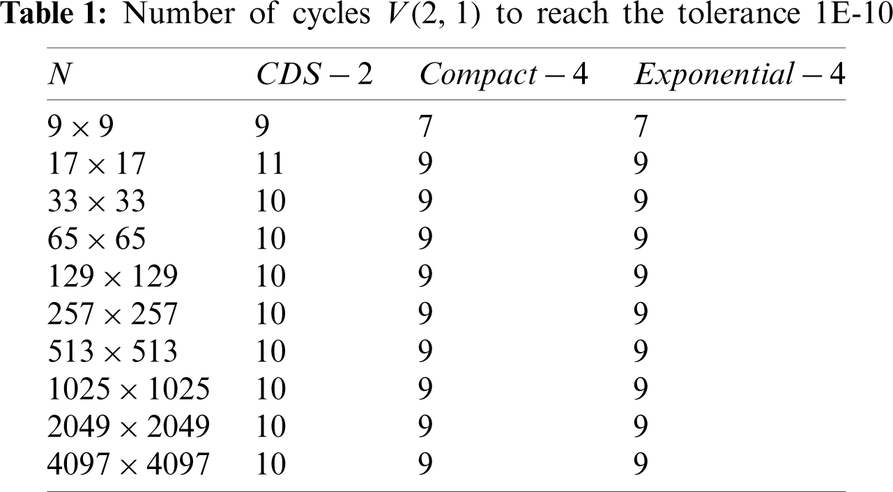
As one can see in Tab. 1, both the Compact −4 and the Exponential −4 methods obtained exactly the same amount of V-cycles. However, a slightly less number of cycles than for the CDS −2, which indicates that fourth orders methods have a slightly better convergence factor.

Tab. 2 shows another analysis only for fourth order methods, considering time computational needed to obtain the same numerical solutions.

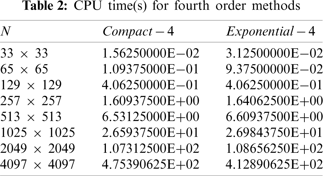
As one can see by Tab. 2, for both methods of fourth order hold very similar computational time. Therefore, it is not possible yet to determine which one is the more efficient.

Given that, Tab. 3 shows the complexity order of the Compact −4 and Exponential −4 methods using multigrid FAS through a geometric curve fitting [5], represented by equation tcpu(N) = cNp. It is known that, according to [6,19], theoretically the p factor must be close to the unit.

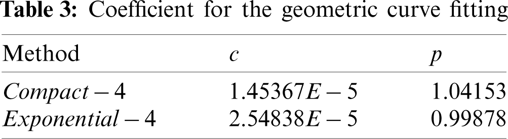
Finally, after applying the curve fitting it is possible to verify that the Exponential −4 method obtained a more adequate complexity factor when obtaining the numerical solutions for the variable of interest U(1/2,1/2), which we defined before in this paper. Note that the Exponential −4 method is not part of the classical compact schemes, so we believe that it is possible to extend its application to obtain numerical solutions for more complex equations, such as the Poisson equations with non-constant or anisotropic coefficients.

6.3 Effect of the Number of Extrapolations

The results present in Tab. 3 show that the complexity factor p of the Exponential −4 method is closer to unity, agreeing with the literature [6]. Therefore, from now on we choose the Exponential −4 method to determine the numerical solutions for the variable U(1/2,1/2) and generate new extrapolated solutions with sixth, eighth and tenth orders of accuracy. In order to do repeated extrapolations using the RRE, the analytical solution was not used, for instance, all the approximations were based on the apparent order pU. For that, one can remember that the true orders of the Exponential −4 method are pm=4,6,8,…, and asymptotic order [17,18] given by pL = 4.

It is possible to observe through Fig. 6 the behavior of the true and apparent orders in the numerical solutions: without performing any extrapolations (m = 0, p0 and Ug,0). When generating the first (m = 1, p1 and Ug,1), second (m = 2, p2 and Ug,2), third (m = 3, p3 and Ug,2) and fourth (m = 4, p4 and Ug,4) Richardson extrapolations.

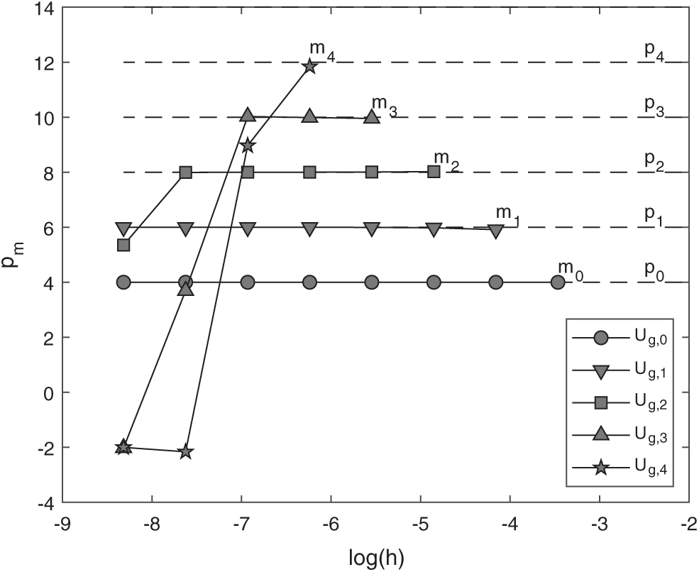
Figure 6: Repeated Richardson extrapolation for U(1/2,1/2)

Observing Fig. 6, we concluded that numerical solutions are found with several precision orders.

The main contribution of this article is to show the possiblity to obtain a new higher accuracy solution without the require to generate a new approximation involving many neighbor points. For this, we start with high-order solution and then apply the post-processing RRE method. This would imply in a large-scale linear systems, so that a computational limitation would happen.

In the Fig. 6 we can observe the influence of the round-off error on the discretization error, which degenerated the orders. Note that the Ug,4 solution is affected by this type of error. With this, we believe that only solutions of tenth order Ug,3 can be considered, excluding the degenerated part.

7  Conclusions

In the present paper, our results were based on a comparison between Compact −4 and Exponential −4 methods with the goal of finding the best efficiency of the fourth order methods when decreasing the discretization error. In addition, without increasing the computational time when solving linear systems of large scale resulting of the discretization of the two-dimensional Poisson equation.

The fourth order methods achieved similar results when considering the number of V(2,1) cycles when reaching the convergence, which indicates that they have a very close convergence factor.

From the curve fitting complexity analysis, the Exponential −4 method obtained a better factor (smaller and closer to the unit) when compared to the Compact −4 method. However, both factors are close to the theoretical expected in the FAS multigrid case.

Given that, using the Exponential −4 method and combining numerical solutions for the U(1/2,1/2) variable in the different grids using the RRE, we obtained new solutions with sixth, eighth and tenth orders of accuracy, as expected by the true orders.

However, it is possible to obtain solutions with superior orders by successive applications of RRE. For that, it is only needed enough different solutions in grids g −1 to generate m repeated extrapolations, i.e., m = g −1.

In practice, our contribution is related to the significant reduction of computational costs during the execution of Engineering projects. It is common that projects are based on numerical solutions of problems that model, for example, heat diffusion. Thus, the strategy presented in this work allows the study of more physical phenomena, ensuring project cost reduction and high reliability.

This work is related to the exclusive approach of the Laplacian operator. However, we believe that extending this technique to the advection-diffusion operator, for example, is not difficult.

Acknowledgement: We would like to acknowledge the graduate program of Numerical Methods in Engineering—PPGMNE from the Federal University of Paraná, Curitiba—PR, Brazil. This study was financed in party by the Coordenação de Aperfeiçoamento de Pessoal de N¡́x0131/¿vel Superior—Brasil (CAPES)—Finance Code 001.

Funding Statement: The authors received no specific funding for this study.

Conflicts of Interest: The authors declare that they have no conflicts of interest to report regarding the present study.

References

 1.  Okoro, F. M., Owoloko, A. E. (2010). Compact finite difference schemes for Poisson equation using direct solver. Journal of Mathematics and Technology, (3), 130–138. http://eprints.covenantuniversity.edu.ng/178/#.YMigwOBKiM9. [Google Scholar]

 2.  Čiegis, R., Suboč, O. (2018). High order compact finite difference schemes on nonuniform grids. Applied Numerical Mathematics, 132, 205–218. DOI 10.1016/j.apnum.2018.06.003. [Google Scholar] [CrossRef]

 3.  Zhang, J., Wang, Y. (2009). Sixth order compact scheme combined with multigrid method and extrapolation technique for 2D Poisson equation. Journal of Computational Physics, 228(1), 137–146. DOI 10.1016/j.jcp.2008.09.002. [Google Scholar] [CrossRef]

 4.  Pandey, P. K. (2013). A higher accuracy exponential finite difference method for the numerical solution of second order elliptic partial differential equations. Journal of Mathematical and Computational Science, 3(5), 1325–1334. http://scik.org/index.php/jmcs/article/view/1217. [Google Scholar]

 5.  Burden, R. L., Faires, J. D. (2016). Numerical analysis, vol. 10. Boston, Massachusetts, USA: Cengage Learning. [Google Scholar]

 6.  Trottenberg, U., Oosterlee, C. W., Schuller, A. (2000). Multigrid. Amsterdam, Netherlands: Elsevier. [Google Scholar]

 7.  Marchi, C. H., Araki, L. K., Alves, A. C., Suero, R., Gonçalves, S. F. T. et al. (2013). Repeated Richardson extrapolation applied to the two-dimensional Laplace equation using triangular and square grids. Applied Mathematical Modelling, 37(7), 4661–4675. DOI 10.1016/j.apm.2012.09.071. [Google Scholar] [CrossRef]

 8.  Marchi, C. H., Novak, L. A., Santiago, C. D., Vargas, A. P. S. (2013). Highly accurate numerical solutions with repeated Richardson extrapolation for 2D Laplace equation. Applied Mathematical Modelling, 37(12–13), 7386–7397. DOI 10.1016/j.apm.2013.02.043. [Google Scholar] [CrossRef]

 9.  Cheney, W., Kincard, D. (1999). Numerical mathematics and computing. USA: Brooks/Cole Publishing. [Google Scholar]

10. Marchi, C. H., Giacomini, F. F., Santiago, C. D. (2016). Repeated Richardson extrapolation to reduce the field discretization error in computational fluid dynamics. Numerical Heat Transfer, Part B: Fundamentals, 70(4), 340–353. DOI 10.1080/10407790.2016.1215702. [Google Scholar] [CrossRef]

11. Marchi, C. H., Silva, A. F. C. (2002). Unidimensional numerical solution error estimation for convergent apparent order. Numerical Heat Transfer, Part B: Fundamentals, 42(2), 167–188. DOI 10.1080/10407790190053888. [Google Scholar] [CrossRef]

12. LeVeque, R. J. (2007). Finite difference methods for ordinary and partial differential equations: Steady-state and time-dependent problems. New Delhi: SIAM. [Google Scholar]

13. Gupta, M. M., Kouatchou, J., Zhang, J. (1997). Comparison of second and fourth order discretizations for multigrid Poisson solvers. Journal of Computational Physics, 132(2), 226–232. DOI 10.1006/jcph.1996.5466. [Google Scholar] [CrossRef]

14. Li, J., Chen, Y. (2008). Computational partial differential equations using MATLAB. London, UK: Chapman and Hall Book. [Google Scholar]

15. Pandey, P. K., Pandey, B. D. (2016). Variable mesh size exponential finite difference method for the numerical solutions of two point boundary value problems. Boletim da Sociedade Paranaense de Matemática, 34(2), 9–27. DOI 10.5269/bspm.v34i2.24599. [Google Scholar] [CrossRef]

16. Pandey, P. K. (2016). Solving two point boundary value problems for ordinary differential equations using exponential finite difference method. Boletim da Sociedade Paranaense de Matemática, 34(1), 45–52. DOI 10.5269/bspm.v34i1.22424. [Google Scholar] [CrossRef]

17. Marchi, C. H., Germer, E. M. (2013). Effect of the CFD numerical schemes on repeated Richardson extrapolation (RRE). Applied & Computational Mathematics, 2, 128. DOI 10.4172/2168-9679.1000128. [Google Scholar] [CrossRef]

18. Marchi, C. H., Martins, M. A., Novak, L. A., Araki, L. K., Pinto, M. A. V. et al. (2016). Polynomial interpolation with repeated Richardson extrapolation to reduce discretization error in CFD. Applied Mathematical Modelling, 40(21–22), 8872–8885. DOI 10.1016/j.apm.2016.05.029. [Google Scholar] [CrossRef]

19. Wesseling, P. (2004). An introduction to multigrid methods. UK: Book News, Inc. https://www.amazon.com/Introduction-Multigrid-Methods-P-Wesseling/dp/1930217080#detailBullets_feature_div. [Google Scholar]

20. Oliveira, M. L., Pinto, M. A. V., Gonçalves, S. F. T., Rutz, G. V. (2018). On the robustness of the xy-zebra-gauss-seidel smoother on an anisotropic diffusion problem. Computer Modeling in Engineering & Sciences, 117(2), 251–270. DOI 10.31614/cmes.2018.04237. [Google Scholar] [CrossRef]

21. Franco, S. R., Gaspar, F. J., Pinto, M. A. V., Rodrigo, C. (2018). Multigrid method based on a space-time approach with standard coarsening for parabolic problems. Applied Mathematics and Computation, 317(4), 25–34. DOI 10.1016/j.amc.2017.08.043. [Google Scholar] [CrossRef]

22. Franco, S. R., Rodrigo, C., Gaspar, F. J., Pinto, M. A. V. (2018). A multigrid waveform relaxation method for solving the poroelasticity equations. Computational and Applied Mathematics, 37(4), 4805–4820. DOI 10.1007/s40314-018-0603-9. [Google Scholar] [CrossRef]

23. Wesseling, P., Oosterlee, C. W. (2001). Geometric multigrid with applications to computacional fluid dynamics. Journal of Computation and Applied Mathematics, 128(1–2), 311–334. DOI https://10.1016/S0377-0427(00)00517-3. [Google Scholar]

24. Santiago, C. D., Marchi, C. H., Souza, L. F. (2015). Performance of geometric multigrid method for coupled two-dimensional systems in CFD. Applied Mathematical Modelling, 39(9), 2602–2616. DOI 10.1016/j.apm.2014.10.067. [Google Scholar] [CrossRef]

25. Stüben, K. (2001). A review of algebraic multigrid. Journal of Computation and Applied Mathematics, 128(1–2), 281–309. DOI 10.1016/S0377-0427(00)00516-1. [Google Scholar] [CrossRef]

26. Suero, R., Pinto, M. A. V., Marchi, C. H., Araki, L. K., Alves, A. C. (2012). Analysis of algebraic multigrid parameters for two-dimensional steady-state heat diffusion equations. Applied Mathematical Modelling, 36(7), 2996–3006. DOI 10.1016/j.apm.2011.09.088. [Google Scholar] [CrossRef]

This work is licensed under a Creative Commons Attribution 4.0 International License, which permits unrestricted use, distribution, and reproduction in any medium, provided the original work is properly cited.