| Computer Modeling in Engineering & Sciences |
DOI: 10.32604/cmes.2021.015747
ARTICLE
Deep Learning-Based Surrogate Model for Flight Load Analysis
1College of Aerospace Science and Engineering, National University of Defense Technology, Changsha, 410073, China
2School of Science, Harbin Institute of Technology, Shenzhen, 518000, China
3National Innovation Institute of Defense Technology, Chinese Academy of Military Science, Beijing, 100071, China
*Corresponding Author: Qinghui Zhang. Email: zhangqh@hit.edu.cn
Received: 10 January 2021; Accepted: 26 April 2021
Abstract: Flight load computations (FLC) are generally expensive and time-consuming. This paper studies deep learning (DL)-based surrogate models of FLC to provide a reliable basis for the strength design of aircraft structures. We mainly analyze the influence of Mach number, overload, angle of attack, elevator deflection, altitude, and other factors on the loads of key monitoring components, based on which input and output variables are set. The data used to train and validate the DL surrogate models are derived using aircraft flight load simulation results based on wind tunnel test data. According to the FLC features, a deep neural network (DNN) and a random forest (RF) are proposed to establish the surrogate models. The DNN meets the FLC accuracy requirement using rich data sources in the FLC; the RF can alleviate overfitting and evaluate the importance of flight parameters. Numerical experiments show that both the DNN-and RF-based surrogate models achieve high accuracy. The input variables importance analysis demonstrates that vertical overload and elevator deflection have a significant influence on the FLC. We believe that synthetic applications of these DL-based surrogate methods show a great promise in the field of FLC.
Keywords: Flight load; surrogate model; deep learning; deep neural network; random forest
Flight loads are forces and moments borne by different components of an aircraft in actual flight states. The flight loads consist of aerodynamic loads, inertial loads, and elastic loads. Flight loads are influenced by complex factors, including working conditions (taking-off, climbing, cruising, maneuvering, landing), atmospheric environment (temperature, air density, gust), and aircraft features (configuration, weight, speed, acceleration).
Flight loads are preconditions of aircraft structural strength design. If the design strength is lower than the actual value, the structure may break down in extreme flight conditions. If the design results are too conservative, a large weight cost has to be paid. Accuracy and efficiency of flight load computation (FLC) directly affect the design quality, progress, and cost, which are of great significance in aircraft design [1,2]. The computation and verification of flight loads are important means of improving aircraft structure design, determining the structural life and reducing the cost. According to different aircraft design stages and accuracy requirements, the FLC methods include numerical analysis, wind tunnel tests, and flight experiments. The latter two methods are expensive; the numerical analysis or its coupling with a wind tunnel test has become the preferred technique for the FLC.
Modern aircraft design involves large loads, large deformations, and multiple transmission paths. Conventional numerical simulation techniques, such as the finite element method, the panel method, and the CFD method require high resolutions and large discretization scales when applied to the FLC. Thus, the load computations are time-consuming, which significantly restricts aircraft research and development. To improve the efficiency of load computation, model order reduction (MOR) of conventional load computation models has attracted research interest [3–6]. The concept of MOR is to reduce the complexity of the original large system and generate a reduced-order model representing the original system [7]. The numerical methods for computing flight loads are based on a complex theoretical mechanism, which is described by a series of elasticity systems of equations, fluid mechanics equations, and the coupling of complex models [8]. An adequate understanding of these mathematical equations and physical mechanism are needed for the MOR.
In recent years, rapid developments in deep learning (DL) have attracted significant attention in the field of aircraft design [9]. The principle of DL is to treat the complex mathematical mechanism as a “black box,” training and validating the model through observation and experimental data to produce surrogate models. DL has achieved remarkable success in image processing, speech recognition, natural language processing, artificial intelligence [9,10]. There are several reasons for the great potential of MOR using DL in the field of aircraft design [7]. First, DL is particularly suitable for exploring complex nonlinear relationships without addressing the mathematical and physical mechanism. Second, DL models have high computational efficiency; there are many mature GPU acceleration technologies that can greatly increase load computation efficiency. Finally, there are rich data available in the field of aircraft design, including wind tunnel test data, flight test data, an data calculated by finite element software. These data can improve the quality of model training and validation to a great extent, and in turn improve the accuracy of the model. We mention that the FLC needs to traverse various conditions combined by speeds, altitudes, plug-in configurations, maneuvering actions, control parameters, etc. Therefore, even for a single typical aircraft, the number of conditions of FLC in every load computation is very large in order not to miss severe load conditions, which consumes a lot of computing time. We refer to the MOR models based on DL as “DL-based surrogate models”.
DL technologies are widely used in the field of international aviation, and have achieved fruitful results in the field of aircraft design. Neural network models of aerodynamics are referred to [11–16]. Neural network models and support vector machine models for aerodynamic force and flight parameters were studied in [17–22]. Learning models for aircraft aerodynamic features at high angles of attack were shown in [23–26]. Research on aerodynamic optimization design using support vector regression methods and kriging models are found in [27,28]. Reed [29] studied structural health monitoring systems based on parametric flight data and artificial neural networks. In aspect of load analysis, the existing research includes landing load analysis [30,31] and load computations [32–36] using neural networks or kriging models. However research on DL-based flight load techniques is limited and requires further development.
This paper studies DL-based surrogate models of FLC to provide a reliable basis for aircraft structure strength design. The surrogate models are established using flight load simulation results from aircraft based on wind tunnel test data. The flight loads are affected by complex factors including body parameters, flight conditions, and control parameters. This paper is focused on symmetrical maneuvers to analyze and verify the effectiveness of the proposed method. In a situation of typical weight, the main flight conditions, altitude, Mach number, speed pressure, are considered in input variables. Furthermore, trim degrees of freedom and trim variables are crucial for the loads in the symmetrical maneuvers, including vertical overload, pitch angular acceleration, angle of attack, elevator deflection, pitch rate. These movement parameters and the flight conditions are set as the input variables of DL surrogate models. In choosing extreme loading situations, the loads at connecting joints of key components of an aircraft are the significant monitoring indicators [37]. Thus, shear force, bending moment and torque at the wing root, wing middle and the root of horizontal tail serve as the output variables in this paper. According to the features of FLC, two DL techniques, deep neural network (DNN) [9,10] and random forest (RF) [38], are proposed to establish the surrogate models. DNN has the advantage of accuracy with sufficient sample data, and meets the accuracy requirement with rich data sources in FLC. RF is not easily overfitted and has excellent generalization ability. Most importantly, RF can evaluate the importance of input variables, which is critical in analyzing the factors affecting flight loads. The surrogate models are tested in typical symmetric flight conditions, with steady pitch and steep pitch. Numerical experiments indicate that both DNN- and RF-based surrogate models achieve high accuracy. The input variable importance analysis demonstrates that vertical overload and elevator deflection have a significant influence and are the primary factors in FLC. Our achievements in this study are summarized in what follows, (1) the input and output variables above are set taking key points of the FLC into full consideration, which were not adopted in the literature, (2) the DNN and RF are selected according to the property of FLC, and (3) the importance analysis on the primary factors for the FLC was not conducted in other studies. It is believed that synthetic applications of DL-based surrogate methods show a great promise in the field of FLC.
The remainder of this paper is organized as follows. Conventional FLC methods are described in Section 2. In Section 3, we introduce DL-based surrogate models using the DNN and RF, and the computation procedure for establishing surrogate models to predict and analyze the flight loads. Numerical verification is presented in Section 4. Conclusions are presented in Section 5.
2 Conventional Flight Load Analysis Methods
The purpose of flight load analysis is to obtain the maximum loads of main aircraft components and the corresponding flight conditions yielding these loads. The aircraft attitude is determined by solving a series of kinetic equations for aircraft, and obtaining the aerodynamic load distribution data, inertial loads, and elastic loads under equilibrium states for the entire aircraft. The maneuvers used in the flight load analysis mainly include symmetrical maneuver flight (pitch maneuver) and asymmetric maneuver flight (roll maneuver, yaw maneuver) [1,2].
First, an analysis axis system was designed. The origin O of the aircraft body axis system is located at the mass center of the aircraft. The Ox-axis is in the symmetry plane of the aircraft, parallel to the fuselage axis, and is positive in the forward direction; the Oz-axis is also in the symmetry plane, perpendicular to the Ox-axis, and positive in the downward direction; the Oy-axis is perpendicular to the symmetry plane, and is positive moving to the right, as shown in Fig. 1.
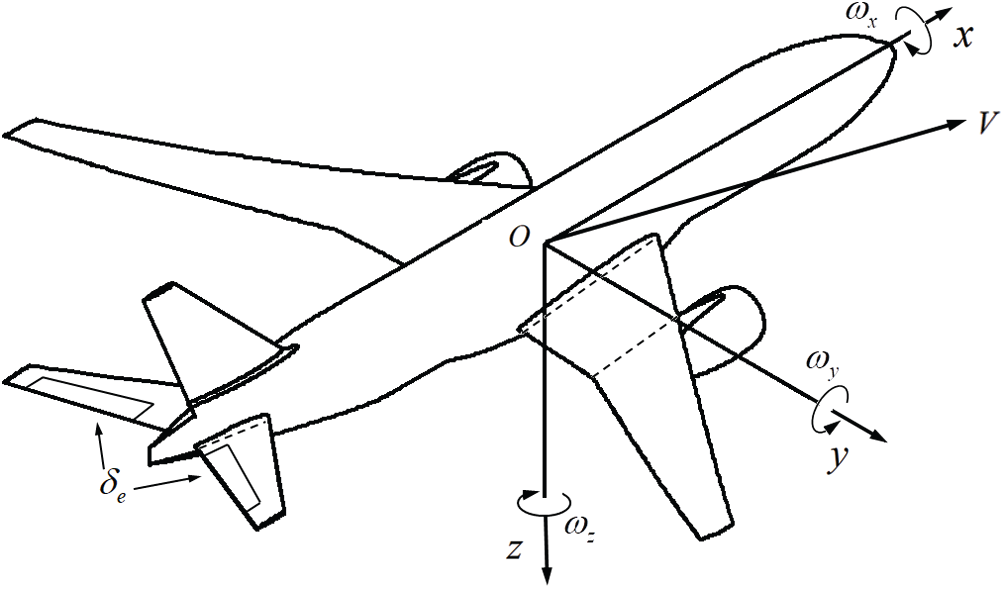
Figure 1: The analysis axis system of an aircraft. V is the direction of velocity,
Determination of flight conditions for load computation
The selection of flight load conditions must cover all flight states within the flight envelope. Usually, standard specifications are chosen based on the type of aircraft; the flight dynamics equations are solved to simulate aircraft maneuvers under the constraints of the specifications. The maneuvers generally include combinations of flight situations, including weights, gravity centers, mass distributions, aerodynamic configurations, speeds, altitudes, engine thrusts, flight control systems, plug-in configurations, maneuvering actions, and control parameters. Based on the maneuvers, the main aircraft maneuver flight parameters are determined as the specific flight load conditions.
Equations of elastic load analysis of entire aircraft
The flight load analysis of elastic aircraft is based on numerically coupling the models of structural data, aerodynamic data, and mass distributions. The flight load data in complicated flight conditions is derived using static finite element analysis methods. The flight load analysis of elastic aircraft is mainly focused on the influence of aircraft structural deformations on aircraft loads. This includes the change in aircraft balance state caused by aerodynamic features and the redistribution of aerodynamic loads caused by structural elastic deformations. The model describing the flight load computations is dominated by a series of equilibrium equations that are based on principles of statics analysis and established by adding aerodynamic forces and considering inertia release theory. The finite element method is used in solving these equations to derive the flight loads. The major equation characterizing static aeroelastic responses is expressed as follows [1,2]:
where
In this paper we mainly study effects of elastic deformations on steady aerodynamic loads. To this end, time independent simplification of (1) is carried out for trim computations. The acceleration vector is obtained by decomposing support degree of freedom (DOF) and remaining DOF of
Computation of flight loads and selection of severe load states
The flight parameters for different conditions of FLC are used as the input of Eq. (1). In other words, under the given maneuvering conditions (composed of known trim degrees of freedom and trim variables), unknown trim degrees of freedom and trim variables can be obtained by solving the balance equation. The distributed load results are obtained using the corresponding finite element analysis software and model, which are integrated to obtain the loads (shear force, bending moment and torque) of different components and typical monitoring sections. By drawing the load envelope for all conditions, severe load results and corresponding states are selected as the basis of structural strength design.
In this paper we use the SOL144 solver to conduct the flight load analysis of an aircraft. The FEM structural mesh model and aerodynamic panel mesh model are constructed in the FLC, as shown in Fig. 2. The aerodynamic panel model is derived by interpolating pressure distribution data produced from wind tunnel tests to the panel mesh. The FEM model is constructed according to structure layout and strength stiffness level of an aircraft. The MSC.Nastran realizes the displacement and equivalent force transportation between aerodynamics and structure. The DOF trim computation of entire aircraft is carried out according to the inertia release theory when solving (1). The structural and aerodynamical data on the trim status is obtained in this way, including loads, deformations, stresses, stability derivatives, control derivatives, pressure distribution, etc.
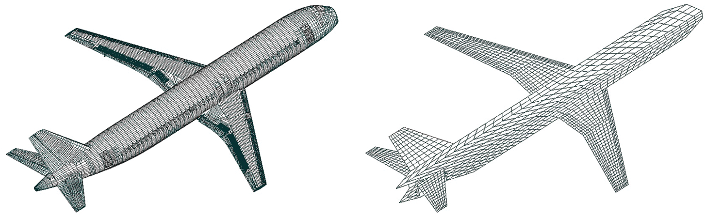
Figure 2: Left: the FEM structural mesh. Right: the aerodynamic panel mesh
Thus, conventional methods of FLC depend heavily on aircraft shape, structural features, flight parameters, external conditions, and flow field information, and have a strong nonlinear relationship with them. These relationships are usually described by coupling a series of complex mathematical and physical equations. Solving these equations requires significant computational resources, which hinders aircraft design quality and schedules. Thus, development of surrogate models of FLC is required. In this paper, DL-based surrogate models of flight loads are developed [5,7]. The models are trained by load data to improve the efficiency and accuracy of load computations, providing a new FLC approach.
3 Surrogate Model Based on Deep Learning for Flight Loads
This section establishes surrogate models for flight load analysis based on two deep learning algorithms, a deep neural network (DNN) and a random forest (RF).
3.1 General Description of Surrogate Model
Let X be the input variable of a load model F, and let L be the loads of interest computed from F according to X. The computation of flight loads can be described generally as follows [9]:
where
A surrogate model views
The surrogate model of
where
The
3.2 Analysis of Input and Output Variables
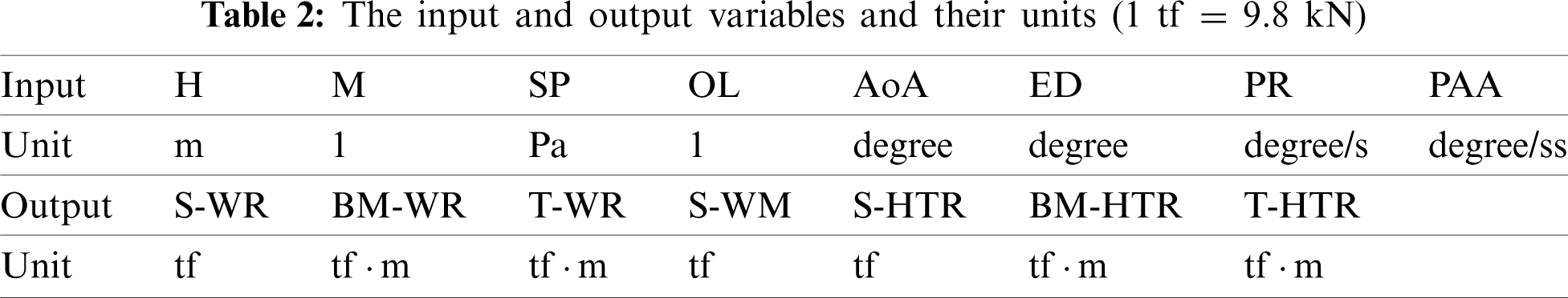
The flight loads are affected by complex factors including body parameters, flight parameters, and control parameters. The loads differ greatly in different flight stages such as take-off, climbing, cruising, gliding down, and landing. Flight parameters such as mass, speed, acceleration, flight attitude, and operation movements influence the flight loads. External flight factors such as temperature, pressure, wind gusts, and atmospheric turbulence also have great impact. In addition, the loads and severe load conditions differ for different parts of the aircraft. For example, the rib and beam of the wing and the frame of the fuselage have different severe load conditions; flight loads are complex and diverse. This paper is focused on symmetrical maneuvers to analyze and verify the effectiveness of the proposed method. In a situation of typical weight, the main flight conditions, altitude (H), Mach number (M), speed pressure (SP), are considered in input variables. The SP is incorporated to clearly identify its relationship with the flight load. Furthermore, the trim DOFs and trim variables are crucial for the loads in the symmetrical maneuvers, including vertical overload (OL), angle of attack (AoA), elevator deflection (ED), pitch rate (PR), and pitch angular acceleration (PAA). These movement parameters and the flight conditions are set as the input variables, i.e.,
To study the most extreme loading conditions, typical sections are selected as monitoring objects. The quantities of interests on these sections, including the bending moment, torque, and shear force, are the key indicators characterizing the flight loads during maneuvering. We choose the root and the middle of the wing and the root of the horizontal tail as the major objects because the most extreme loads generally occur in these sections [37]. The shear force, bending moment and torque in these sections serve as the output variables L to develop the surrogate model, whose values are the integrated force and the moment relative to the reference point.
We introduce two typical deep learning algorithms, a deep neural network and a random forest, to establish the surrogate model
A deep neural network (DNN) [9,10] can be considered as a neural network with one input layer, one output layer, and many hidden layers. Each neuron belongs to different layers. The layers are connected by chains. The signal propagates unidirectionally from the input layer to the output layer; the whole network is equivalent to a directed acyclic graph. Specifically, we multiply the response value of the ith layer, Z(l), by an associated wight matrix W(l), and then add a bias term b(l). The summation is mapped by a nonlinear activation function
and so on.
In this paper we use a so-called residual neural network [10], which is an improvement of the conventional DNN above and has been shown to perform better in many cases. A residual network is converted from the simple network by inserting a shortcut connection, and does not directly fit the target, but fits the residual. A multilayer network with a hop layer connection is generally referred to as a residual block. In this paper, we construct a residual block with two FC layers and one shortcut connection, as shown in Fig. 3 Right. The mathematical expression of the ith residual block is expressed as follows:
where X is the initial input. The whole residual network consists of many residual blocks and a linear transformations. A residual network with M residual blocks is expressed as
where
The network updates the parameters using back propagation algorithm until the desired results are achieved. In the back propagation algorithm, parameters are updated based on gradients of loss function with respect to the parameters, and these gradients are computed using an adaptive moment method, Adam et al. [39].
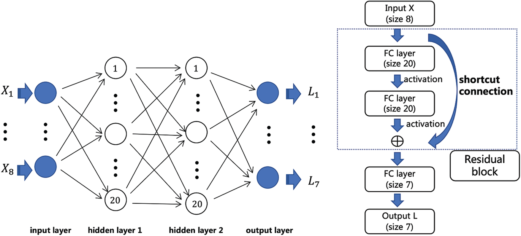
Figure 3: Left: An example of four-layer FC network we use in the experiments, which contains two hidden layers, and each hidden layer has 20 neurons. The dimension sizes of input and output are 8 and 7, respectively. Right: A residual neural network with only one residual block
The residual network better fits high-dimensional functions. The fitting ability is not affected by network width. The residual network can significantly increase training speed and pre-precision of deep networks, break the symmetry of networks, reduce network degradation, and improve network characterization ability.A residual DNN is accurate with sufficient sample data, and meets the accuracy requirements with rich data sources in FLC.
A random forest is a machine learning method that uses decision trees to train samples and predict objectives [38]. A random forest is composed of many decision trees (also known as classification trees or regression trees), as shown in Fig. 4, and each decision tree is constructed to establish a model that predicts the value of target variables according to multiple input variables.
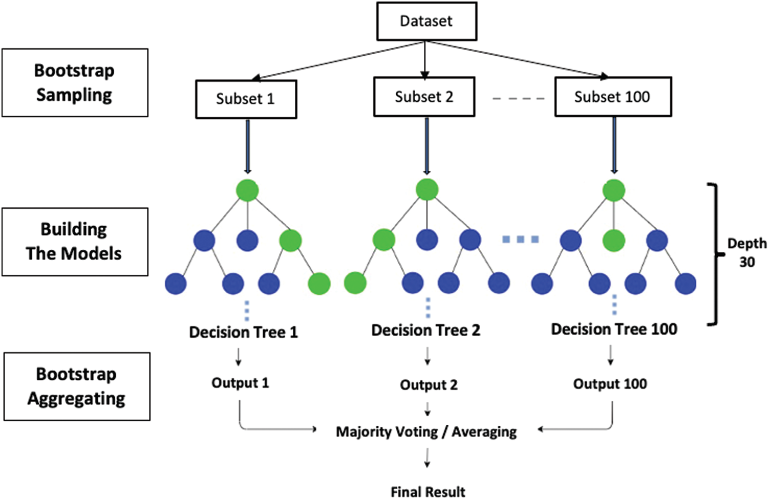
Figure 4: The random forest. The data set is divided into 100 subsets by bootstrap sampling, and the model (decision tree) is established on each subset. Finally, through the bagging, the final result is obtained according to the output of each decision tree
A random forest is established using the bagging (bootstrap aggregating) algorithm to vote the decision tree. In statistics, the bootstrap is a kind of ensemble technology that trains classifiers by selecting new data sets from the original data set through sampling with replacement. The number of selected objects will accounts for approximately 63% of the source samples; the remaining 37% of the samples are used to test the generalization ability of the constructed model. We randomly select n training samples from the whole sample set
In our computations, we use a RF regressor. The number of trees in the forest is 100, and the maximum depth of tree is 30. The number of samples is also 24619, from which 17233 samples are selected randomly for the bootstrap sample. 100 trees are built based on 100 bootstrap sample sets obtained from these 17233 samples. The quality of a split is measured by the mean square error (MSE), and the variance reduction serves as the feature selection criterion. The load regression prediction of an input is computed as the mean regression predictions of the trees in the forest.
An RF is not easily overfitted and has excellent generalization ability. Most important, an RF can evaluate the importance of input variables, which is critical in analyzing factors affecting flight loads.
The FLC procedure using DL-based surrogate models is described as follows:
1. analyze the factors affecting FLC and key monitoring components to set input and output variables;
2. compute the data used to train and validate the surrogate models using conventional flight load simulation algorithms based on wind tunnel test data;
3. train and validate the DNN and RF surrogate models;
4. compare the accuracy of the surrogate models;
5. identify the importance of input variables to determine the main factors affecting FLC;
6. adjust Steps (1) and (2) according to Steps (4) and (5) and repeat the procedure until a reasonable result is produced, comparable to results from conventional methods.
4 Numerical Analysis and Verification
Using an example aircraft, we perform FLC using the proposed deep-learning surrogate models, DNN and RF. We test the accuracy of the two surrogate models and analyze their load prediction results through finite element analysis. The importance of the input variables is evaluated using the RF model to identify the main factors influencing loads.
4.1 Aircraft Parameters and Flight Load Data
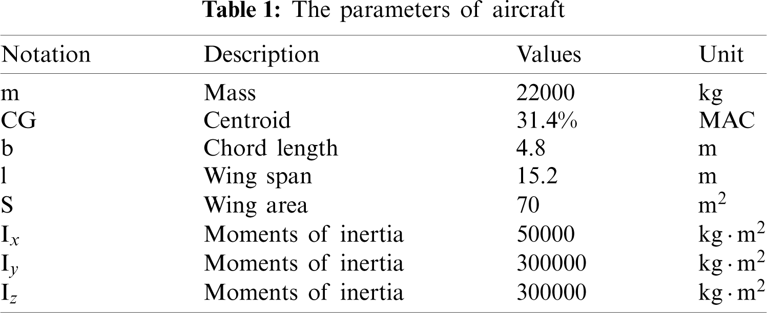
We consider a high-speed and high-maneuverability aircraft with a conventional configurations. The wings have a double beam wing box structure. The specific parameters of the aircraft are shown in Tab. 1. We consider typical symmetric flight attitudes, maneuvers of steady pitch and steep pitch. The data used to develop the surrogate model is generated from wind tunnel experiments and finite element software. Specifically, the aerodynamic data and pressure distribution data are from the results of wind tunnel experiments. The flight load software, MSC.Flightloads, is employed to establish the coupling model of finite element structural model, aerodynamic model, and mass model, and to load the external wind tunnel data. Then, a static aeroelastic solver, SOL144, in the MSC nastran is used to solve the problem. The 24619 data pairs in Section 3.2 with different values of input and output variables are produced in this way to train and test the surrogate models in the numerical tests below. Each data pair contains 8 input variables and 7 output variables, respectively. We save the data as a matrix of
As analyzed in Section 3.2, the input variables include the flight altitude (H), Mach number (M), speed pressure (SP), vertical overload (OL), angle of attack (AoA), elevator deflection (ED), pitch rate (PR), and pitch angular acceleration (PAA), which are the main factors affecting flight loads, see (4). We choose the root and the middle of the wing and the root of the horizontal tail as the major objects because the most extreme loads generally occur in these sections. The shear force (S), bending moment (BM), and torque (T) at the wing root (WR) and horizontal tail root (HTR), and the shear of the wing middle (WM) serve as the output variables L to develop the surrogate model. The input and output variables and their units of DL-based surrogate models are summarized in Tab. 2.
4.2 Description of DNN and RF Surrogate Models
We present major parameters in the DNN and RF surrogate models, proposed in Sections 3.3 and 3.4. For the DNN, we use the residual neural network [9,10]. The structure of the DNN includes the number of hidden layers, the number of nodes in each layer, the activation function, and the training function. These parameters have a vital influence on the accuracy and training speed of the DNN. The network structure used in the numerical test consists of several residual blocks, each of which contains two full connection layers and one residual item. In each residual block, there are ten neurons in the total junction layer, and seven neurons in the output layer. The introduction of residual terms helps to alleviate the difficulty caused by the disappearance of gradients, and makes the network easier to train. The activation function is the
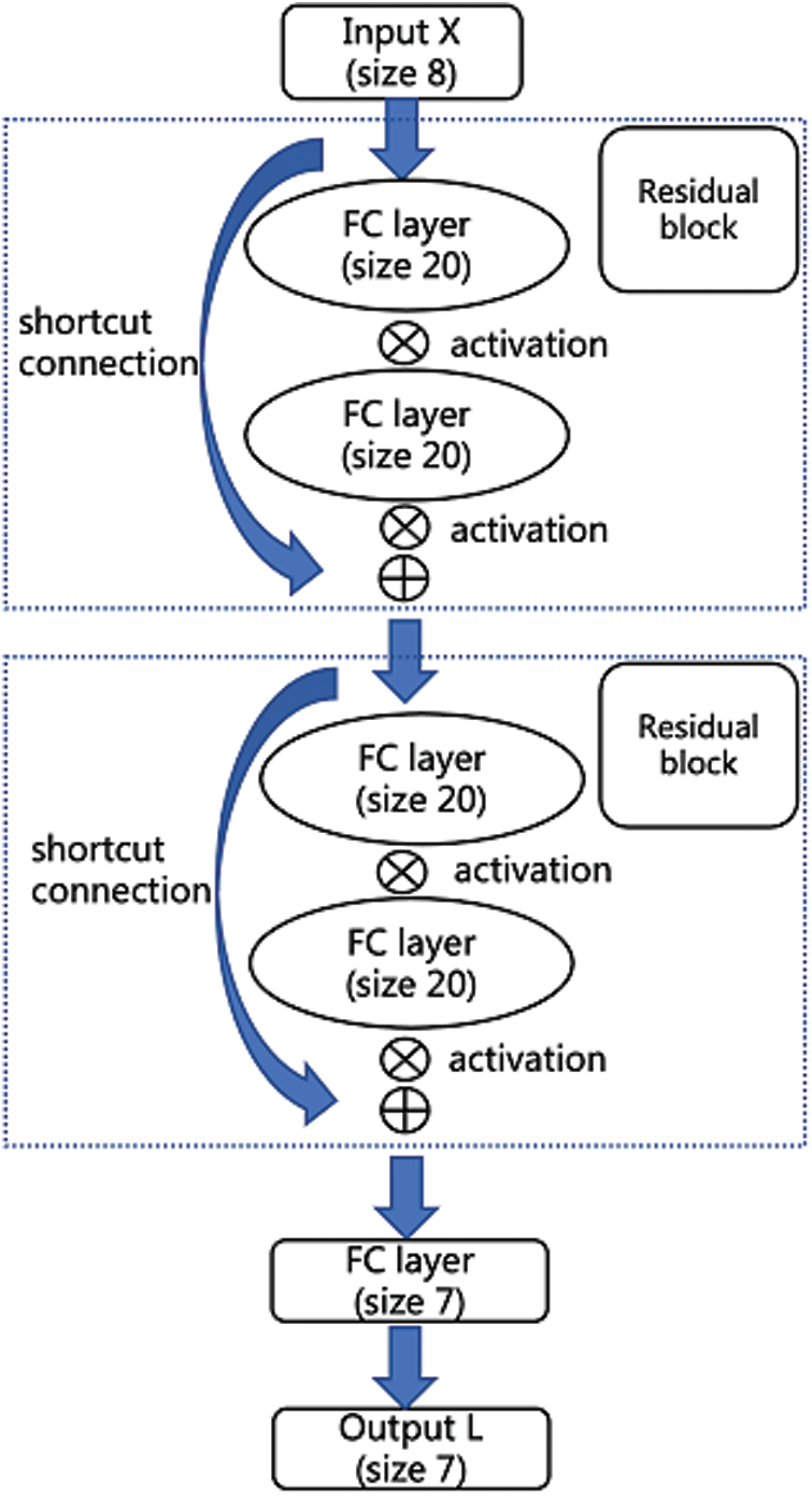
Figure 5: The figure shows a network with two blocks and an output linear layer. Each block consists of two fully-connected layers with size 20 and a residual connection. The activation function here is
A total of 24619 data pairs are used to construct the DNN surrogate model, of which 17233 pairs are used to train the model. The model is adjusted according to the error computed from these pairs. A total of 3693 data pairs are used to judge when the training is finished. The training is stopped when these pairs are used to continue training but the network structure is not greatly improved. Finally, a total of 3693 data pairs are used to test the model errors of the surrogate model. The tanh function, whose range is
A random forest is a meta estimator that fits a number of classifying decision trees on different sub-samples of the data set and uses averaging to improve the predictive accuracy and control overfitting [38]. In our model, the number of trees in the forest is 100; the maximum depth of the tree is 30. Bootstrap samples are used when building trees; 17233 and 7386 of the 24619 data pairs are used to train the model and test the errors, respectively. We note that the RF does not need to normalize the initial data sets.
4.3 Accuracy of Computation and Model Analysis
We employ mean square error (MSE) and coefficients of determination R2 to examine the accuracy of models, defined as follows:
where Yi and
According to the results in Tabs. 3 and 4, R2 values for both models are both close to 1, indicating that the surrogate models demonstrate the high fitting accuracy. The MSE of the RF model is 0.03267 for the training set, which is better than 0.05963 in the DNN model. However, the MSE of the RF in the test set is 0.08412, which is larger than 0.05995 in the DNN model. The MSEs in the DNN model for the training, validation, and test sets are similar; the DNN model is more stable. The DNN model is easier to train because residual terms are introduced. However, the RF model does not need to normalize the data in training, and can identify the importance of input variables.
The predicted shear force (S), bending moment (BM), and torque (T) of the DNN and RF surrogate models are presented in Figs. 6 and 7. The horizontal coordinate is the actual value the vertical coordinate is the predicted value. The closer the sample points are to the straight line y = x, the closer the predicted results are to the actual result. The high accuracy of both surrogate models for the computation of flight loads is verified.
To demonstrate the efficiency of the DNN and RF surrogate models, we compare them with the conventional neural network method. The neural network has been applied to aeronautical areas quite early, as reviewed in the Introduction, see [11,16,17,19,23,29,32,34,35] for example. We use a neural network with 80 neurons for the FLC; the number of neurons is as many as that in the DNN model. The MSE and R2 for the training, validation, and test sets for the neural network model are presented in Tab. 5. It is shown in Tab. 5 that compared with the neural network model, the accuracy of proposed DNN and RF surrogate models is significantly improved.
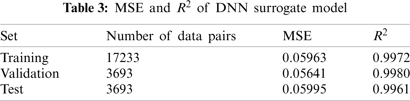


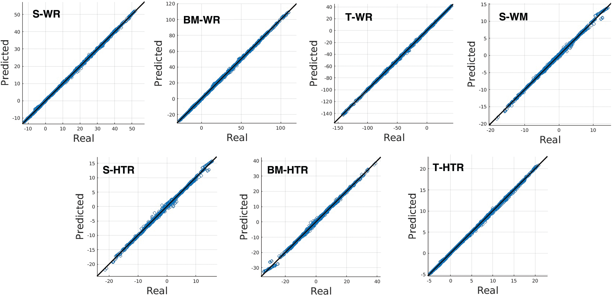
Figure 6: The predicted shear force (S), bending moment (BM), and torque (T) of DNN surrogate model. The top four are at the wing root (WR) and wing middle (WM), while the bottom three are at horizontal tail root (HTR). The closer the sample points are to the straight line y = x, the closer the predicted results are to the real result
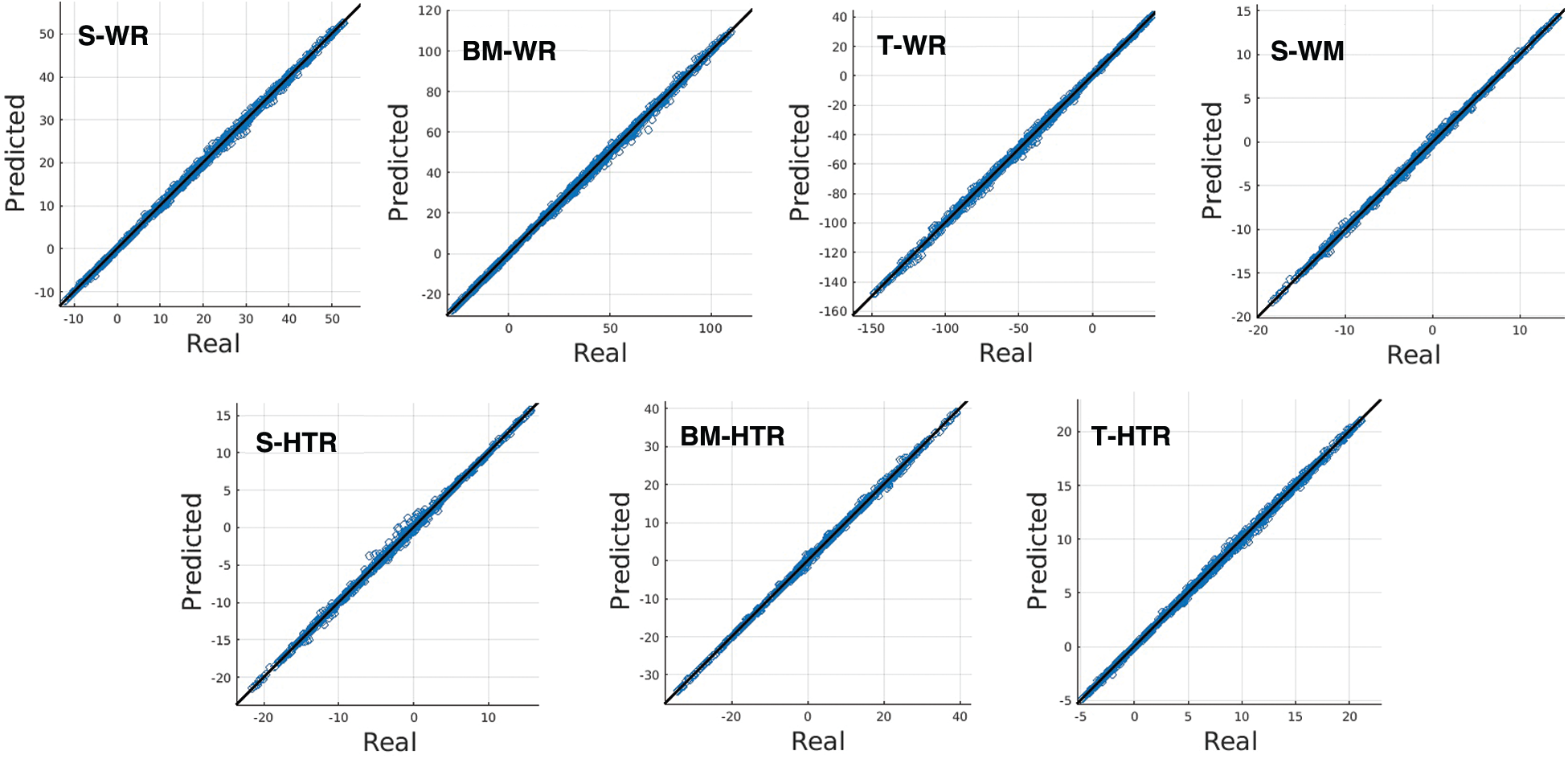
Figure 7: The predicted shear force (S), bending moment (BM), and torque (T) of RF surrogate model. The top four are at the wing root (WR) and wing middle (WM), while the bottom three are at horizontal tail root (HTR). The closer the sample points are to the straight line y = x, the closer the predicted results are to the real result
4.4 Importance Analysis of Input Variables
We introduce many variables to train the surrogate models; their influences on flight loads are different. Thus, identifying the importance of different variables is critical in the analysis of loads. The main factors are instructive in developing more efficient load computation approaches. We apply the RF to identify the importance of input variables; this is an advantages of RF over other deep learning techniques, including the DNN. In the RF, the importance of a variable is computed as the (normalized) total reduction of the criterion brought by that variable. It is also known as the Gini importance. The importance of a variable is calculated as follows. A baseline metric, defined by scoring, is evaluated on a (potentially different) dataset defined by X. A variable column from the validation set is permuted and the metric is evaluated again. The permutation importance is defined as the difference between the baseline metric and the metric from permutating the feature column. The importance of the input variables computed using the RF is presented in Tab. 6. It can be seen from Tab. 6 that the importance of the input variables ranked from high to low is as follows: vertical overload (OL), elevator deflection (ED), angle of attack (AoA), Mach number (M), speed pressure (SP), pitch angular acceleration (PAA), flight altitude (H), and pitch rate (PR). The vertical overload and elevator deflection are the main factors in the load computation.

This paper studied deep learning-(DL) based surrogate models of flight load computations (FLC). A deep neural network (DNN) and a random forest (RF) were proposed to establish the surrogate models according to the features of FLC. The DNN meets the accuracy requirement of FLC with rich data sources in FLC; the RF can alleviate overfitting and evaluate the importance of flight parameters. The data used to train and validate the DL surrogate models were derived using aircraft flight load simulation results based on wind tunnel test data. Numerical experiments showed that both the DNN-and RF-based surrogate models achieve high accuracy. The input variable importance analysis was conducted to identify the main factors in FLC. This paper was focused on typical symmetric flight conditions, steady pitch and steep pitch, to test the surrogate models. Additional flight conditions, such as roll maneuvers, yaw maneuvers, and severe load conditions within the flight envelope will be investigated in future research.
Acknowledgement: The authors wish to express their appreciation to the anonymous reviewers for their helpful suggestions which greatly improved the presentation of this paper.
Funding Statement: This research was partially supported by the Natural Science Foundation of China under Grant 91730305 and Guangdong Provincial Natural Science Foundation of China under Grant 2017B030311001.
Conflicts of Interest: The authors declare that they have no conflicts of interest to report regarding the present study.
1. MSC.Nastran (2008). Quick reference guide. MSC Software, Santa Ana, CA. [Google Scholar]
2. Shan, H. (2015). Research of determining flight load envelope of aircraft using reduced-order models (Master Thesis) (in Chinese). [Google Scholar]
3. Choi, Y., Boncoraglio, G., Anderson, S., Farhat, C. (2020). Gradient-based constrained optimization using a database of linear reduced-order models. Journal of Computational Physics, 423, 109787. DOI 10.1016/j.jcp.2020.109787. [Google Scholar] [CrossRef]
4. Kapteyn, M., Knezevic, D., Huynh, D., Tran, M., Willcox, K. (2020). Data-driven physics-based digital twins via a library of component-based reduced-order models. International Journal for Numerical Methods in Engineering, 53(10), 3073. DOI 10.1002/nme.6423. [Google Scholar] [CrossRef]
5. Jirasek, A., Cummings, R. M. (2012). Reduced order modeling of x-31 wind tunnel model aerodynamic loads. AIAA, 219, 2010–4693. DOI 10.1016/j.ast.2011.10.014. [Google Scholar] [CrossRef]
6. Crowell, A. R., McNamara, J. J., Kecskemety, K. M., Goerig, T. (2012). A reduced order aerothermodynamic modeling framework for hypersonic aerothermoelasticity, pp. 2010–2969. Reston, VA: AIAA. [Google Scholar]
7. Mohamed, K. M. (2018). Machine learning for model order reduction. Cham: Springer. [Google Scholar]
8. Liu, Y., Wan, Z., Li, Q., Zhang, Q. (2020). A corrected nearest neighbor transportation method of aerodynamic force for fluid-structure interactions. International Journal of Numerical Analysis and Modeling, 17, 746–765. [Google Scholar]
9. Goodfellow, I., Bengio, Y., Courville, A. (2016). Deep learning. Cambridge, MA: MIT Press. [Google Scholar]
10. He, K., Zhang, X., Ren, S., Sun, J. (2016). Deep residual learning for image recognition. Proceedings of the IEEE Conference on Computer Vision and Pattern Recognition, pp. 770–778. Las Vegas, NV. [Google Scholar]
11. Steck, J. E., Rokhsaz, K. (1997). Some applications of artificial neural networks in modeling of nonlinear aerodynamics and flight dynamics, pp. 97–338. Reno, NV: AIAA. [Google Scholar]
12. Kutz, J. N. (2017). Deep learning in fluid dynamics. Journal of Fluid Mechanics, 814, 1–4. DOI 10.1017/jfm.2016.803. [Google Scholar] [CrossRef]
13. Ling, J., Kurzawski, A., Templeton, J. (2016). Reynolds averaged turbulence modeling using deep neural networks with embedded invariance. Journal of Fluid Mechanics, 807, 155–166. DOI 10.1017/jfm.2016.615. [Google Scholar] [CrossRef]
14. Zhang, T., Qian, W., Zhou, Y., Lei, H., Shao, Y. (2019). Preliminary thoughts on the combination of artificial intelligence and aerodynamics. Advances in Aeronautical Science and Engineering, 10, 1–11. DOI 10.16615/j.cnki.1674-8190.2019.01.001 (In Chinese). [Google Scholar] [CrossRef]
15. Ladicky, L., Jeong, S., Solenthaler, B., Pollefeys, M., Gross, M. (2015). Data-driven fluid simulations using regression forests. ACM Transaction Graphics, 34(6), 1–99. DOI 10.1145/2816795.2818129. [Google Scholar] [CrossRef]
16. Gomec, F., Canibek, M. (2017). Aerodynamic database improvement of aircraft based on neural networks and genetic algorithms. 7th European Conference for Aeronautics and Space Sciences, pp. 2017–2226. Milan, Italy. [Google Scholar]
17. Secco, N., Mattos, B. (2017). Artifificial neural networks to predict aerodynamic coeffificients of transport airplanes. Aircraft Engineering and Aerospace Technology: An International Journal, 89, 211–230. DOI 10.1108/AEAT-05-2014-0069. [Google Scholar] [CrossRef]
18. Zhang, Y., Sung, W., Mavris, D. (2018). Application of convolutional neural network to predict airfoil lift coefficient, pp. 1903–2018. Reston, VA: AIAA. [Google Scholar]
19. Wallach, R., Mattos, B., Girardi, R., Curvo, M. (2012). Aerodynamic coefficient prediction of a general transport aircraft using neural network, pp. 658–2006. Reston, VA: AIAA. [Google Scholar]
20. He, L., Qian, W., Wang, Q., Chen, H., Yang, J. (2019). Applications of machine learning for aerodynamic characteristics modeling. Acta Aerodynamics Sinica, 37, 470–479. DOI 10.7638/kqdlxxb-2019.0033 (In Chinese). [Google Scholar] [CrossRef]
21. Chen, H., He, L., Qian, W., Wang, S. (2020). Multiple aerodynamic coeffificient prediction of airfoils using a convolutional neural network. Symmetry, 12(4), 544. DOI 10.3390/sym12040544. [Google Scholar] [CrossRef]
22. Yilmaz, E., German, B. J. (2017). A convolutional neural network approach to training predictors for airfoil performance. 18th AIAA/ISSMO Multidisciplinary Analysis and Optimization Conference, 2017. Denver, Colorado. [Google Scholar]
23. Ignatyev, D., Khrabrov, A. (2018). Experimental study and neural network modeling of aerodynamic characteristics of canard aircraft at high angles of attack. Aerospace, 5(1), 26. DOI 10.3390/aerospace5010026. [Google Scholar] [CrossRef]
24. Ignatyev, D., Khrabrov, A. (2015). Neural network modeling of unsteady aerodynamic characteristics at high angles of attack. Aerospace Science and Technology, 41(2), 106–115. DOI 10.1016/j.ast.2014.12.017. [Google Scholar] [CrossRef]
25. Chen, Y. L. (2012). Modeling of longitudinal unsteady aerodynamics at high angle-of-attack based on support vector machine. Proceeding of the 8th International Conference on Natural Computation, pp. 431–435, New York: IEEE. [Google Scholar]
26. Wang, Q., Qian, W., He, K. (2015). Unsteady aerodynamic modeling at high angle of attack using support vector machines. Chinese Journal of Aerodynamics, 28(3), 659–668. DOI 10.1016/j.cja.2015.03.010. [Google Scholar] [CrossRef]
27. Andrés, E., Salcedo-Sanz, S., Monge, F., Pérez-Bellido, A. M. (2012). Effificient aerodynamic design through evolutionary programming and support vector regression algorithms. Expert Systems with Applications, 39(12), 10700–10708. DOI 10.1016/j.eswa.2012.02.197. [Google Scholar] [CrossRef]
28. Jeong, S., Murayama, M., Yamamoto, K. (2005). Efficient optimization design method using kriging model. Journal of Aircraft, 42(2), 413–420. DOI 10.2514/1.6386. [Google Scholar] [CrossRef]
29. Reed, S. (2008). Indirect aircraft structural monitoring using artificial neural networks. The Aeronautical Journal, 112(1131), 251–265. DOI 10.1017/S0001924000002190. [Google Scholar] [CrossRef]
30. Holmes, G., Sartor, P., Reed, S., Southern, P., Worden, K. et al. (2016). Prediction of landing gear loads using machine learning techniques. Structural Health Monitoring, 15(5), 568–582. DOI 10.1177/1475921716651809. [Google Scholar] [CrossRef]
31. Jeong, S., Lee, K., Ham, J., Kim, J., Cho, J. (2020). Estimation of maximum strains and loads in aircraft landing using artifcial neural network. International Journal of Aeronautical and Space Sciences, 21(1), 117–132. DOI 10.1007/s42405-019-00204-2. [Google Scholar] [CrossRef]
32. Cooper S. B., DiMaio D. (2018). Static load estimation using artificial neural network: Application on a wing rib. Advances in Engineering Software, 125(1), 113–125. DOI 10.1016/j.advengsoft.2018.01.007. [Google Scholar] [CrossRef]
33. Halle, M., Thielecke, F. (2018). Local model networks applied to flight loads estimation. 31st Congress of the International Council of the Aeronautical Science. Belo Horizonte, Brazil. [Google Scholar]
34. Allen, M. J., Dibley, R. P. (2003). Modeling aircraft wing loads from flight data using neural networks, pp. 2003–2120. Washington, DC: NASA/TM. [Google Scholar]
35. Wada, D., Sugimoto, Y. (2017). Inverse analysis of aerodynamic loads from strain information using structural models and neural networks. Sensors and Smart Structures Technologies for Civil, Mechanical, and Aerospace Systems, 101680. Portland, Oregon. [Google Scholar]
36. Kim, D., Pechaud, L. (2001). Improved methodology for the prediction of the empennage maneuver in-flight loads of a general aviation aircraft using neural networks. Embry-Riddle Aeronautical Univ Daytona Beach Fl. [Google Scholar]
37. Niu, M. C. Y. (1999). Airframe structural design: Practical design information and data on aircraft structures. 2nd ed. Northridge, CA: Adaso Adastra Engineering Center. [Google Scholar]
38. Breiman, L. (2001). Random forests. Machine Learning, 45(1), 5–32. DOI 10.1023/A:1010933404324. [Google Scholar] [CrossRef]
39. Kingma, D. P., Ba, J. (2014). Adam: A method for stochastic optimization. arXiv: 1412.6980. [Google Scholar]
 | This work is licensed under a Creative Commons Attribution 4.0 International License, which permits unrestricted use, distribution, and reproduction in any medium, provided the original work is properly cited. |