| Computer Modeling in Engineering & Sciences |
DOI: 10.32604/cmes.2021.015224
ARTICLE
Solution of Modified Bergman Minimal Blood Glucose-Insulin Model Using Caputo-Fabrizio Fractional Derivative
1Department of Mathematics, AMITY School of Applied Science, AMITY University Rajasthan, Jaipur, 302022, India
2Department of Mathematics and Computer Sciences, Cankaya University, Balgat, 06530, Turkey
3Institute of Space Sciences, Magurele-Bucharest, R76900, Romania
4School of Liberal Studies, Dr. B.R. Ambedkar University Delhi, Delhi, 110006, India
*Corresponding Author: Manvendra Narayan Mishra. Email: manvendra.mishra22187@gmail.com
Received: 2 December 2020; Accepted: 20 February 2021
Abstract: Diabetes is a burning issue in the whole world. It is the imbalance between body glucose and insulin. The study of this imbalance is very much needed from a research point of view. For this reason, Bergman gave an important model named-Bergman minimal model. In the present work, using Caputo-Fabrizio (CF) fractional derivative, we generalize Bergman’s minimal blood glucose-insulin model. Further, we modify the old model by including one more component known as diet D(t), which is also essential for the blood glucose model. We solve the modified model with the help of Sumudu transform and fixed-point iteration procedures. Also, using the fixed point theorem, we examine the existence and uniqueness of the results along with their numerical and graphical representation. Furthermore, the comparison between the values of parameters obtained by calculating different values of t with experimental data is also studied. Finally, we draw the graphs of G(t), X(t), I(t), and D(t) for different values of
Keywords: Bergman minimal model; blood glucose; Caputo-Fabrizio fractional derivative; uniqueness and existence; fractional calculus
These days, Mathematical modeling is turning out to be a vital tool in mathematical science. Since it translates real-world problems into mathematical language and after applying the necessary methods, we again translate the results into real-world languages to forecast the objective. In every field, modeling is being used to achieve or predict the future prospective. In recent years, modeling is being used with another important but less interactive field of mathematics–-Fractional Calculus (see [1–8]). We have studied several problems and their solutions by ordinary calculus methods, but sometimes fractional calculus gives us better results to describe the model than the old one. Fractional calculus has several real-world applications. A few of them are Fractional conservation of mass, Groundwater flow problem, Time-space fractional diffusion equation models, Acoustical wave equations, Fractional Schrdinger equation in quantum theory, etc. (see [9–22]).
Nowadays, diabetes is turning out to be a fatal disease. The imbalance between body glucose and insulin causes diabetes. It is categorized into two types. Type-I diabetes is more severe than Type-II. According to a survey, Type-I and Type-II diabetes sufferers are one ratio nine. So, the study of this imbalance was very much needed from a research point of view. For this reason, Bergman gave an important model named-Bergman minimal model (see [23–27]).
Riemann-Liouville and Caputo introduced the initial concept of fractional calculus. But they use a singular kernel in their definition. However, Caputo and Fabrizio recently found specific systems related to material heterogeneities that cannot be well connected with Riemann-Liouville or Caputo derivative. Because of that, Caputo and Fabrizio introduced a new fractional derivative operator involving a non-singular kernel. Due to its memory and non-singularity property, this operator is used to study different models of engineering, science, and bio-mathematical fields. In general, we get more reliable results while using this operator than others for more details of applications of Caputo-Fabrizio derivative (see [28–45]).
Apart from changing the model to fractional-order, we also include the Diet factor in the model that describes the effect of meals on the glucose level. The generalize of Bergman’s minimal blood glucose-insulin model gives us a more precise and detailed prediction about the problem.
1.1 The Caputo-Fabrizio Fractional Differential Operator [46–48]
Definition 1: Suppose
If,
also,
One thing is to be noted here that the Caputo-Fabrizio operator has an exponent differential coefficient. We know that the exponential function has no singularity which, means the derivative exists at every point of the territory. So CF operator gives better results in its domain, see [49–56].
Definition 2: The fractional integral of the function h(t) of order
Remark 1: From the above equation, we conclude that the fractional integral of order
Based on the above relation, Nieto and Losada defined the following operator;
1.2 Sumudu Transform of Caputo-Fabrizio Operator [57,58]
Suppose f(t) be a function whose Caputo-Fabrizio derivative occurs, hence the Sumudu Transform of Caputo-Fabrizio fractional differential coefficient of f(t) is defined below:
The whole paper is divided into six sections. Section first introduces fractional calculus and mathematical modeling with its brief history. The second section describes the Bergman model’s fractional exponent and an overview of the fractional modified minimal model. The third section discusses the existence and uniqueness of the modified mathematical model with the help of the Caputo-Fabrizio operator. Section 4 is devoted to the solution of the model by using the Sumudu Transform operator. Section 5 deals with numerical solutions along with graphical representations of the modified Bergman model. In section 6, we have concluded our findings.
2.1 Bergman Model of Fractional Order
Here, we are going to discuss the Bergman model of fractional order. In this model, we consider a glucose chamber and plasma insulin which is inherent to carry out across the isolated chamber to control the final glucose intake. This model, asserts that this is good to satisfy specific validation criteria with minimum parameters. This system is efficient in describing the gesture of interactivity of blood sugar and insulin. In the presented model, we suppose that G(t) is the imbalance of plasma glucose cluster and I(t) is the free plasma insulin cluster, from their initial values. The model was
with starting conditions G(0) = G0, X(0) = X0, and I(0) = I0.
2.2 Overview of Fractional Modified Minimal Model
Here, we redefined the structure of the previous model. We made some changes in the model and added few parameters. As we have, ‘Diet’ having significant effect on the glucose level. Now the changed structured Bergman modified system has been described in the following equations-
Here one thing is to be noted that
This model can be a tool in search of an artificial pancreas. But, unfortunately, it also adopts the problems with the glucose-minimal model. Here, G(t)–-blood glucose cluster, X(t)–-aftermath of effective insulin, I(t)–-blood insulin cluster, D(t)–-infusion of exogenous glucose, u(t)–-insulin distribution function, Gb–-initial blood glucose cluster, Ib–-initial blood insulin cluster, V1–-insulin issuance volume, n–-fractional fading rate of insulin, p1–-insulin free glucose dispensation rate, p2–-active insulin dispensation rate and p3–-the increase in absorption capacity caused by insulin.
3 Existence of the Solutions of Described Model
Define K1, K2, K3, K4 and their relations with variables.
Proof: Since the system is
Here one thing is to be noted that
Then by definition stated by Nieto, we get
Now let us suppose the kernels are given as
Show that K1, K2, K3 and K4 satisfies the Lipchitz condition.
Proof: At first, we shall show this for K1. Suppose G and G1 are any functions, so
Similarly, we can have
Now consider the recursive formula
Now suppose that the deviation amid two successive terms is
Now
But K1 satisfies Lipchitz condition so,
Similarly, we have
Establish that Bergman Minimal Model with Fractional-order is a minimum system of sugar insulin dynamics.
Proof: Using the recursive technique, we have
Hence the existence of results is verified, which is continuous too. Now we get
So,
Similarly, we have
From the above, it is clear that,
Now,
Now taking
On behalf of the above equations, we can state that the solution of the system exists.
To show the uniqueness of results, we suppose that other sets of results exist for the system specified from Eqs. (46) to (49) such that
taking norm both sides, we get
using Lipchitz condition, we obtain
which is valid for all n, so
similarly
Hence, it claims uniqueness of the system.
4 Result of the Model by Using Sumudu Transform
Considering the system has various equations so it can be challenging to find the exact results. For this, we will adopt the iterative technique together with the Sumudu Transform. Now take Sumudu Transform either sides, side of Eq. (15)
At this moment, take inverse Sumudu Transform on both ends, we have-
Similarly, we have from Eqs. (16)–(18)
Then we get the following recurrent form from the above
The result is obtained by
For numerical solution, we use the values given below by the experiment defined in [59,60].
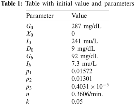
By using the above-defined values, we can easily determine the numerical results for the defined model. In that analysis, we found the numerical result by using the sumudu transform. We found the result for some different
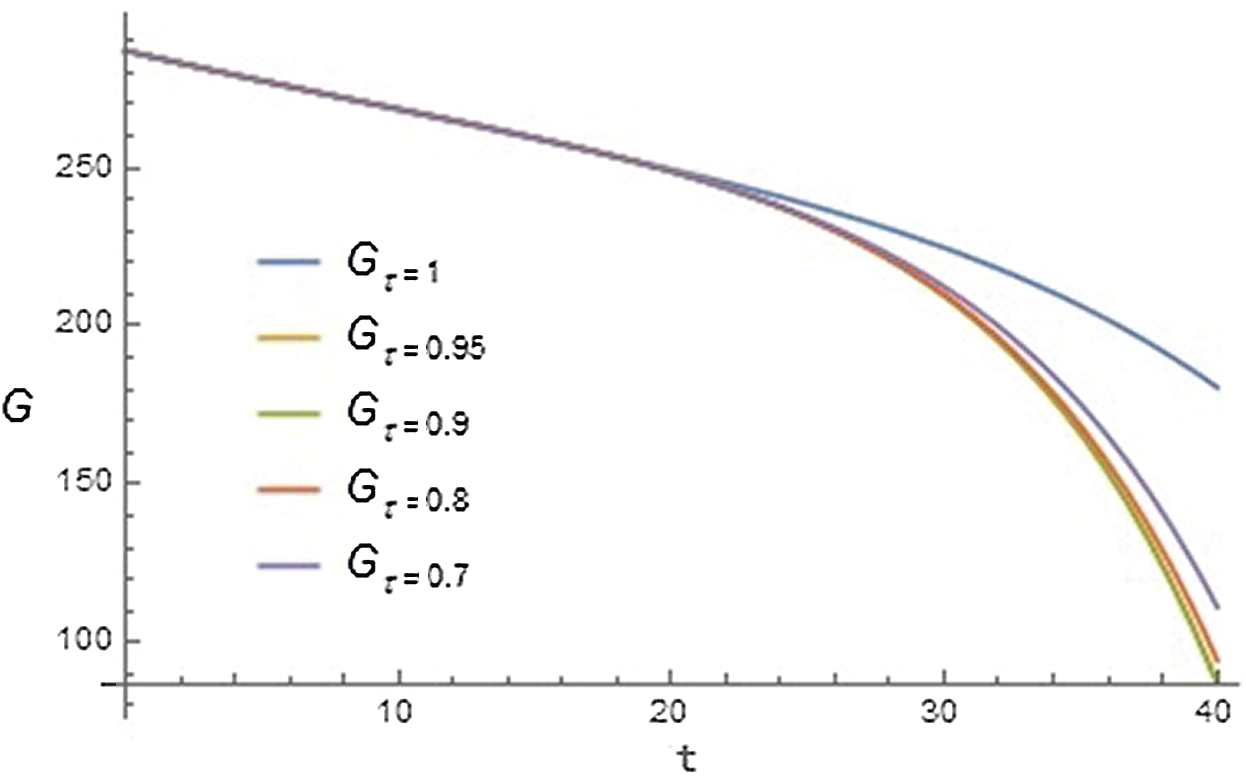
Figure 1: Graph of blood glucose cluster (G) with respect to time t for different values of
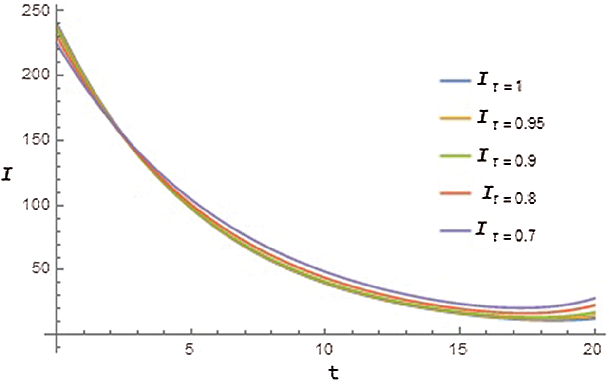
Figure 2: Graph of blood insulin cluster (I) with respect to time t for different values of
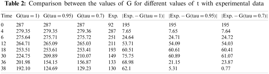
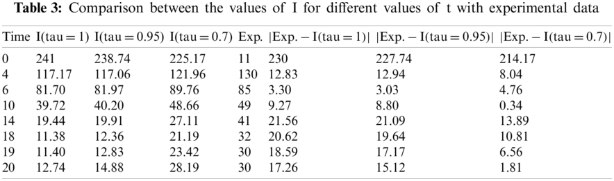
Furthermore, it has been observed from Tabs. 2 and 3, that the values obtained for G and I with linear order have more error than fractional order. So we can see that the fractional model with Caputo-Fabrizio operator gives better results in contrast to linear model, and our model defined the real-world problem in a better manner.
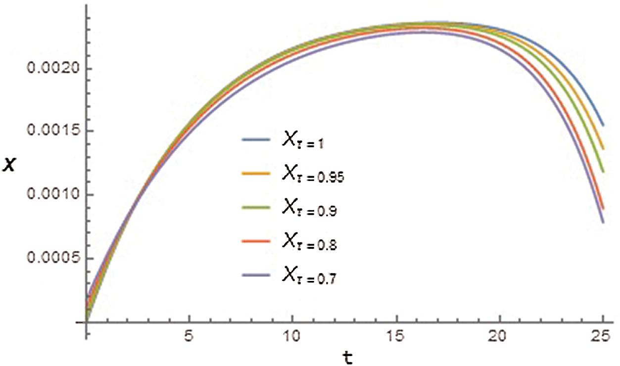
Figure 3: Graph of aftermath of effective insulin (X) with respect to time t for different values of
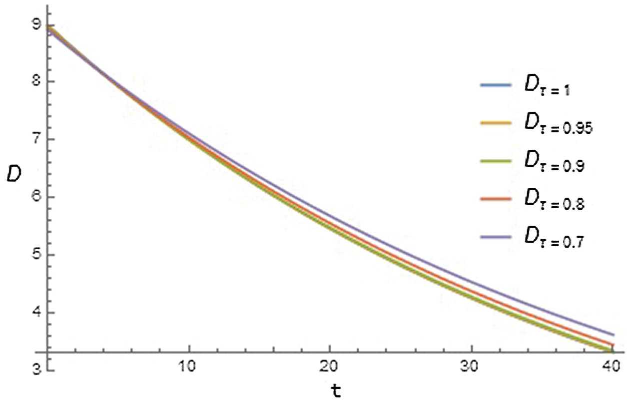
Figure 4: Graph of infusion of exogenous glucose (D) with respect to time t for different values of
The presented work strives to explain the presence and oneness of the Modified Bergman Minimal Model that is stretched out by Caputo-Fabrizio fractional differential coefficient in the frame of reference of sugar and insulin quantity in blood. From the obtained results, it is clear that the fractional model error reduces compared to integer order. Thus, we get nearby results of a set-up that displays the aftermath of time on the concentrations G(t), X(t), I(t), and D(t). As in future work, we can generalize the model or compare the results using various differential operators.
Acknowledgement: The authors wish to express their appreciation to the reviewers for their helpful suggestions which greatly improved the presentation of this paper.
Funding Statement: The authors received no specific funding for this study.
Conflicts of Interest: The authors declare that they have no conflicts of interest to report regarding the present study.
1. Podlubny, I. (1998). Fractional differential equations: An introduction to fractional derivatives, fractional differential equations, to methods of their solution and some of their applications. USA: Elsevier, Academic Press. [Google Scholar]
2. Caputo, M. (1967). Linear models of dissipation whose Q is almost frequency independent-II. Geophysical Journal International, 13(5), 529–539. DOI 10.1111/j.1365-246X.1967.tb02303.x. [Google Scholar] [CrossRef]
3. Chaurasia, V. B. L., Dubey, R. S. (2013). Analytical solution for the generalized time-fractional telegraph equation. Fractional Differential Calculus, 3(1), 21–29. DOI 10.7153/fdc-03-02. [Google Scholar] [CrossRef]
4. Miller, K. S., Ross, B. (1993). An introduction to the fractional calculus and fractional differential equations. New York: John Wiley and Sons. [Google Scholar]
5. Chaurasia, V. B. L., Dubey, R. S. (2011). Analytical solution for the differential equation containing generalized fractional derivative operators and Mittag–Leffler-type function. ISRN Applied Mathematics, 2011(3). DOI 10.5402/2011/682381. [Google Scholar] [CrossRef]
6. Kilbas, A. A., Srivastava, H. M., Trujillo, J. J. (2006). Theory and applications of fractional differential equations, pp. 204, Amsterdam, Netherlands: Elsevier. [Google Scholar]
7. Yang, A. M., Zhang, Y. Z., Cattani, C., Xie, G. N., Rashidi, M. M. et al. (2014). Application of local fractional series expansion method to solve Klein–Gordon equations on cantor sets. Abstract and Applied Analysis, 2014(1), 1–6. DOI 10.1155/2014/372741. [Google Scholar] [CrossRef]
8. Baleanu, D., Diethelm, K., Scalas, E., Trujillo, J. J. (2012). Models and numerical methods, series on complexity. Singapore, New Jersey, London and Hong Kong: World Scientific Publishing Company. DOI 10.1142/10044. [Google Scholar] [CrossRef]
9. Alkahtani, B. S. T., Atangana, A. (2016). Analysis of non-homogeneous heat model with new trend of derivative with fractional order. Chaos, Solitons and Fractals, 89(11), 566–571. DOI 10.1016/j.chaos.2016.03.027. [Google Scholar] [CrossRef]
10. Yang, X. J., Machado, J. T., Cattani, C., Gao, F. (2017). On a fractal LC-electric circuit modeled by local fractional calculus. Communications in Nonlinear Science and Numerical Simulation, 47, 200–206. DOI 10.1016/j.cnsns.2016.11.017. [Google Scholar] [CrossRef]
11. Jajarmi, A., Baleanu, D., Sajjadi, S. S., Asad, J. H. (2019). A new feature of the fractional Euler–Lagrange equations for a coupled oscillator using a non-singular operator approach. Frontiers in Physics, 7, 196. DOI 10.3389/fphy.2019.00196. [Google Scholar] [CrossRef]
12. Debbouche, A., Torres, D. F. (2014). Approximate controllability of fractional delay dynamic inclusions with nonlocal control conditions. Applied Mathematics and Computation, 243(10), 161–175. DOI 10.1016/j.amc.2014.05.087. [Google Scholar] [CrossRef]
13. Alkahtani, B. S., Algahtani, O. J., Dubey, R. S., Goswami, P. (2017). Solution of fractional oxygen diffusion problem having without singular kernel. Journal of Nonlinear Sciences and Applications, 10(1), 1–9. DOI 10.22436/jnsa.010.01.28. [Google Scholar] [CrossRef]
14. Dubey, R. S., Alkahtani, B. S. T., Atangana, A. (2015). Analytical solution of space-time fractional Fokker-Planck equation by homotopy perturbation Sumudu transform method. Mathematical Problems in Engineering, 2015(2), 1–7. DOI 10.1155/2015/780929. [Google Scholar] [CrossRef]
15. Yang, X. J., Srivastava, H. M., Cattani, C. (2015). Local fractional homotopy perturbation method for solving fractal partial differential equations arising in mathematical physics. Romanian Reports in Physics, 67(3), 752–761. [Google Scholar]
16. Atangana, A., Alabaraoye, E. (2013). Solving a system of fractional partial differential equations arising in the model of HIV infection of CD4+ cells and attractor one-dimensional Keller–Segel equations. Advances in Difference Equations, 2013(1), 1–14. DOI 10.1186/1687-1847-2013-94. [Google Scholar] [CrossRef]
17. Odibat, Z., Momani, S. (2008). Modified homotopy perturbation method: Application to quadratic Riccati differential equation of fractional order. Chaos, Solitons and Fractals, 36(1), 167–174. DOI 10.1016/j.chaos.2006.06.041. [Google Scholar] [CrossRef]
18. Shaikh, A. S., Shaikh, I. N., Nisar, K. S. (2020). A mathematical model of COVID-19 using fractional derivative: Outbreak in India with dynamics of transmission and control. Advances in Difference Equations, 2020(1), 1–19. DOI 10.1186/s13662-020-02834-3. [Google Scholar] [CrossRef]
19. Chaurasia, V. B. L., Dubey, R. S., Belgacem, F. B. M. (2012). Fractional radial diffusion equation analytical solution via Hankel and Sumudu transforms. International Journal of Mathematics in Engineering Science and Aerospace, 3(2), 179–188. [Google Scholar]
20. Baleanu, D., Jajarmi, A., Sajjadi, S. S., Mozyrska, D. (2019). A new fractional model and optimal control of a tumor-immune surveillance with non-singular derivative operator. Chaos: An Interdisciplinary Journal of Nonlinear Science, 29(8), 83127. DOI 10.1063/1.5096159. [Google Scholar] [CrossRef]
21. Jajarmi, A., Ghanbari, B., Baleanu, D. (2019). A new and efficient numerical method for the fractional modeling and optimal control of diabetes and tuberculosis co-existence. Chaos: An Interdisciplinary Journal of Nonlinear Science, 29(9), 93111. DOI 10.1063/1.5112177. [Google Scholar] [CrossRef]
22. Yildiz, T. A., Jajarmi, A., Yildiz, B., Baleanu, D. (2020). New aspects of time fractional optimal control problems within operators with non-singular kernel. Discrete and Continuous Dynamical Systems–S, 13(3), 407. DOI 10.3934/dcdss.2020023. [Google Scholar] [CrossRef]
23. Bergman, R. N., Ider, Y. Z., Bowden, C. R., Cobelli, C. (1979). Quantitative estimation of insulin sensitivity. American Journal of Physiology–Endocrinology and Metabolism, 236(6), 667–677. DOI 10.1152/ajpendo.1979.236.6.E667. [Google Scholar] [CrossRef]
24. Bergman, R. N., Cobelli, C. (1980). Minimal modeling, partition analysis, and the estimation of insulin sensitivity. Federation Proceedings, 39(1), 110–115. [Google Scholar]
25. Alkahtani, B. S., Alkahtani, O. J., Dubey, R. S., Goswami, P. (2017). The solution of modified fractional Bergman’s minimal blood glucose-insulin model. Entropy, 19(5), 114. DOI 10.3390/e19050114. [Google Scholar] [CrossRef]
26. Dubey, R. S., Belgacem, F. B. M., Goswami, P. (2016). Homotopy perturbation approximate solutions for Bergman’s minimal blood glucose-insulin model. Fractional Geometry and Nonlinear Analysis in Medicine and Biology, 2(3), 6. DOI 10.15761/FGNAMB.1000140. [Google Scholar] [CrossRef]
27. Fisher, M. E. (1991). A semiclosed-loop algorithm for the control of blood glucose levels in diabetics. IEEE Transactions on Biomedical Engineering, 38(1), 57–61. DOI 10.1109/10.68209. [Google Scholar] [CrossRef]
28. Alshabanat, A., Jleli, M., Kumar, S., Samet, B. (2020). Generalization of Caputo-Fabrizio fractional derivative and applications to electrical circuits. Frontiers in Physics, 8(64). DOI 10.3389/fphy.2020.00064. [Google Scholar] [CrossRef]
29. Aydogan, S. M., Baleanu, D., Mohammadi, H., Rezapour, S. (2020). On the mathematical model of rabies by using the fractional Caputo-Fabrizio derivative. Advances in Difference Equations, 2020(1), 1–21. DOI 10.1186/s13662-020-02798-4. [Google Scholar] [CrossRef]
30. Baleanu, D., Mohammadi, H., Rezapour, S. (2020). Analysis of the model of HIV-1 infection of CD4+ CD4 + T-cell with a new approach of fractional derivative. Advances in Difference Equations, 2020(1), 1–17. DOI 10.1186/s13662-020-02544-w. [Google Scholar] [CrossRef]
31. Moore, E. J., Sirisubtawee, S., Koonprasert, S. (2019). A Caputo-Fabrizio fractional differential equation model for HIV/AIDS with treatment compartment. Advances in Difference Equations, 2019(1), 1–20. DOI 10.1186/s13662-019-2138-9. [Google Scholar] [CrossRef]
32. Saleem, M. U., Farman, M., Ahmad, M. O., Rizwan, M. (2017). Control of an artificial human pancreas. Chinese Journal of Physics, 55(6), 2273–2282. DOI 10.1016/j.cjph.2017.08.030. [Google Scholar] [CrossRef]
33. Farman, M., Saleem, M. U., Ahmed, M. O., Ahmad, A. (2018). Stability analysis and control of the glucose insulin glucagon system in humans. Chinese Journal of Physics, 56(4), 1362–1369. DOI 10.1016/j.cjph.2018.03.037. [Google Scholar] [CrossRef]
34. Khalid, A., Khan, I., Khan, A., Shafie, S. (2015). Unsteady MHD free convection flow of Casson fluid past over an oscillating vertical plate embedded in a porous medium. Engineering Science and Technology: An International Journal, 18(3), 309–317. DOI 10.1016/j.jestch.2014.12.006. [Google Scholar] [CrossRef]
35. Sheikh, N. A., Ali, F., Saqib, M., Khan, I., Jan, S. A. A. et al. (2017). Comparison and analysis of the Atangana–Baleanu and Caputo–Fabrizio fractional derivatives for generalized Casson fluid model with heat generation and chemical reaction. Results in Physics, 7(2), 789–800. DOI 10.1016/j.rinp.2017.01.025. [Google Scholar] [CrossRef]
36. Owolabi, K. M., Atangana, A., Akgul, A. (2020). Modelling and analysis of fractal-fractional partial differential equations: Application to reaction-diffusion model. Alexandria Engineering Journal, 59(4), 2477–2490. DOI 10.1016/j.aej.2020.03.022. [Google Scholar] [CrossRef]
37. Owolabi, K. M., Shikongo, A. (2020). Mathematical modelling of multi-mutation and drug resistance model with fractional derivative. Alexandria Engineering Journal, 59(4), 2291–2304. DOI 10.1016/j.aej.2020.02.014. [Google Scholar] [CrossRef]
38. Shaikh, A., Tassaddiq, A., Nisar, K. S., Baleanu, D. (2019). Analysis of differential equations involving Caputo–Fabrizio fractional operator and its applications to reaction-diffusion equations. Advances in Difference Equations, 2019(1), 1–14. DOI 10.1186/s13662-019-2115-3. [Google Scholar] [CrossRef]
39. Tarasov, V. E. (2019). Caputo–Fabrizio operator in terms of integer derivatives: Memory or distributed lag. Computational and Applied Mathematics, 38(3), 1–15. DOI 10.1007/s40314-019-0767-y. [Google Scholar] [CrossRef]
40. Qureshi, S., Rangaig, N. A., Baleanu, D. (2019). New numerical aspects of Caputo–Fabrizio fractional derivative operator. Mathematics, 7(4), 374. DOI 10.3390/math7040374. [Google Scholar] [CrossRef]
41. Abro, K. A., Memon, A. A., Abro, S. H., Khan, I., Tlili, I. (2019). Enhancement of heat transfer rate of solar energy via rotating Jeffrey nano fluids using Caputo–Fabrizio fractional operator: An application to solar energy. Energy Reports, 5(20), 41–49. DOI 10.1016/j.egyr.2018.09.009. [Google Scholar] [CrossRef]
42. Ali, F., Sheikh, N. A., Khan, I., Nisar, K. S. (2020). Caputo–Fabrizio fractional derivatives modeling of transient MHD Brinkman nano liquid: Applications in food technology. Chaos, Solitons and Fractals, 131(12), 109489. DOI 10.1016/j.chaos.2019.109489. [Google Scholar] [CrossRef]
43. Atangana, A., Khan, M. A. (2020). Modeling and analysis of competition model of bank data with fractal-fractional Caputo–Fabrizio operator. Alexandria Engineering Journal, 59(4), 1985–1998. DOI 10.1016/j.aej.2019.12.032. [Google Scholar] [CrossRef]
44. Khan, M. A., Alfiniyah, C., Alzahrani, E. (2020). Analysis of dengue model with fractal-fractional Caputo–Fabrizio operator. Advances in Difference Equations, 2020(1), 1–23. DOI 10.1186/s13662-020-02881-w. [Google Scholar] [CrossRef]
45. Gomez-Aguilar, J. F. (2018). Fundamental solutions to electrical circuits of non-integer order via fractional derivatives with and without singular kernels. The European Physical Journal Plus, 133(5), 197. DOI 10.1140/epjp/i2018-12018-x. [Google Scholar] [CrossRef]
46. Caputo, M., Fabrizio, M. (2015). A new definition of fractional derivative without singular kernel. Progress in Fractional Differentiation and Applications, 1(2), 73–85. DOI 10.12785/pfda/010201. [Google Scholar] [CrossRef]
47. Shrahili, M., Dubey, R. S., Shafay, A. (2020). Inclusion of fading memory to Banister model of changes in physical condition. Discrete and Continuous Dynamical Systems-S, 13(3), 881–888. DOI 10.3934/dcdss.2020051. [Google Scholar] [CrossRef]
48. Srivastava, H. M., Shanker Dubey, R., Jain, M. (2019). A study of the fractional order mathematical model of diabetes and its resulting complications. Mathematical Methods in the Applied Sciences, 42(13), 4570–4583. DOI 10.1002/mma.5681. [Google Scholar] [CrossRef]
49. Singh, J., Kumar, D., Baleanu, D. (2020). A new analysis of fractional fish farm model associated with Mittag–Leffler-type kernel. International Journal of Biomathematics, 13(2), 2050010. DOI 10.1142/S1793524520500102. [Google Scholar] [CrossRef]
50. Baleanu, D., Wu, G. C. (2019). Some further results of the laplace transform for variable order fractional difference equations. Fractional Calculus and Applied Analysis, 22(6), 1641–1654. DOI 10.1515/fca-2019-0084. [Google Scholar] [CrossRef]
51. Baleanu, D., Etemad, S., Rezapour, S. (2020). A hybrid Caputo fractional modeling for thermostat with hybrid boundary value conditions. Boundary Value Problems, 2020(1), 1–16. DOI 10.1186/s13661-020-01361-0. [Google Scholar] [CrossRef]
52. Odibat, Z., Baleanu, D. (2019). A Linearization based approach of homotopy analysis method for non-linear time fractional parabolic PDEs. Mathematical Methods in the Applied Sciences, 42(18), 7222–7232. DOI 10.1002/mma.5829. [Google Scholar] [CrossRef]
53. Velasco, M. P., Usero, D., Jiménez, S., Váquez, L., Váquez-Poletti, J. L. et al. (2020). About some possible implementations of the fractional calculus. Mathematics, 8(6), 893. DOI 10.3390/math8060893. [Google Scholar] [CrossRef]
54. Jajarmi, A., Yusuf, A., Baleanu, D., Inc, M. (2020). A new fractional HRSV model and its optimal control: A non-singular operator approach. Physica A: Statistical Mechanics and Its Applications, (547), 123860. DOI 10.1016/j.physa.2019.123860. [Google Scholar] [CrossRef]
55. Shahmorad, S., Ostadzad, M. H., Baleanu, D. (2020). A Tau-like numerical method for solving fractional delay integro-differential equations. Applied Numerical Mathematics, 151(1–2), 322–336. DOI 10.1016/j.apnum.2020.01.006. [Google Scholar] [CrossRef]
56. Dizicheh, A. K., Salahshour, S., Ahmadian, A., Baleanu, D. (2020). A novel algorithm based on the Legendre wavelets spectral technique for solving the Lane-Emden equations. Applied Numerical Mathematics, (153), 443–456. DOI 10.1016/j.apnum.2020.02.016. [Google Scholar] [CrossRef]
57. Katatbeh, Q. D., Belgacem, F. B. M. (2011). Applications of the Sumudu transform to fractional differential equations. Nonlinear Studies, 18(1), 99–112. [Google Scholar]
58. Dubey, R. S., Goswami, P., Belgacem, F. B. M. (2014). Generalized time-fractional telegraph equation analytical solution by Sumudu and Fourier transforms. Journal of Fractional Calculus and Applications, 5(2), 52–58. [Google Scholar]
59. Khan, M. W., Abid, M., Khan, A. Q. (2019). Fractional order Bergman’s minimal model-A better representation of blood glucose-insulin system. International Conference on Applied and Engineering Mathematics, pp. 68–73. Taxila, Pakisthan, IEEE. DOI 10.1109/ICAEM.2019.8853741. [Google Scholar] [CrossRef]
60. Pacini, G., Bergman, R. N. (1986). MINMOD: A computer program to calculate insulin sensitivity and pancreatic responsivity from the frequently sampled intravenous glucose tolerance test. Computer Methods and Programs in Biomedicine, 23(2), 113–122. DOI 10.1016/0169-2607(86)90106-9. [Google Scholar] [CrossRef]
 | This work is licensed under a Creative Commons Attribution 4.0 International License, which permits unrestricted use, distribution, and reproduction in any medium, provided the original work is properly cited. |