| Computer Modeling in Engineering & Sciences |
DOI: 10.32604/cmes.2021.015885
ARTICLE
Reliability Analysis of Piled Raft Foundation Using a Novel Hybrid Approach of ANN and Equilibrium Optimizer
1Department of Civil Engineering, National Institute of Technology, Patna, Bihar, India
2Faculty of Civil Engineering, Transportation Engineering and Architecture, University of Maribor, Maribor, Slovenia
*Corresponding Author: Pijush Samui. Email: pijush@nitp.ac.in
Received: 22 January 2021; Accepted: 31 May 2021
Abstract: In many civil engineering projects, Piled Raft Foundations (PRFs) are usually preferred where the incoming load from the superstructures is very high. In geotechnical engineering practice, the settlement of soil layers is a critical issue for the serviceability of the structures. Thus, assessment of risk associated with the structures corresponding to the maximum allowable settlement of soils needs to be carried out in the design phase. In this study, reliability analysis of PRF based on settlement criteria is performed using a high-performance hybrid soft computing model. The new approach is an integration of the artificial neural network (ANN) and a recently developed meta-heuristic algorithm called equilibrium optimizer (EO). The concept of reliability index was used to explore the feasibility of a newly constructed hybrid model of ANN and EO (i.e., ANN-EO) against the conventional approach of calculating the probability of failure of PRF. Experimental results show that the proposed ANN-EO attained the most accurate prediction with R2 = 0.9914 and RMSE = 0.0518 in the testing phase, which are significantly better than those obtained from conventional ANN, multivariate adaptive regression splines, and genetic programming, including the ANN optimized with particle swarm optimization developed in this study. Based on the experimental results of different settlement values, the newly constructed ANN-EO is very potential to analyze the risk associated with civil engineering structures. Also, the present study would significantly contribute to the knowledge pool of reliability studies related to piled raft systems because the works of literature on reliability analysis of piled raft systems are relatively scarce.
Keywords: Risk analysis; soil; meta-heuristic optimization; particle swarm optimization
Piled Raft Foundations (PRFs) have gained popularity among the engineering fraternity where it is necessary to transmit a large amount of superstructure load to the ground [1]. If normal pile foundations are adopted to carry a large incoming load, the depth of the piles becomes too large and it may prove to be uneconomical [2,3]. On the other hand, if only raft foundations are used, the resultant settlements are usually too great which may impair the serviceability performance of the structure. In such a scenario, PRF may be chosen to carry the superstructure load where the combined presence of raft and piles will efficiently carry the incoming load and restrict the settlement within the permissible limits. Therefore, the installation of PRF allows an increase in the load capacity and reduction of settlements in a very economical way.
Griffith et al. [4] modeled rafts as a two-dimensional thin plate, in which the authors considered the piles a as one-dimensional rod element and soil as a vertical spring at each node. Later, this model was modified to take into account the effects of multilayered nonhomogeneous soil [5]. Poulos [6] modeled piles as interactive springs and soil as an elastic continuum. Brzakala et al. [7] performed the probabilistic analysis of raft foundations resting on layered subsoil. In the said study, the author performed a numerical analysis based on the finite element method coupled with stochastic versions of the perturbation and the Neumann expansion methods. Russo [8] modeled the piles as a nonlinear spring on the elastic continuum. Also, the idea of Winkler spring was successfully applied for modelling the piles as coupled spring [9]. Niandou et al. [3] developed a numerical model of a piled raft foundation to describe how the soil-structure interaction can be influenced by horizontal soil variability. Alkinani et al. [1] investigated the distribution of load under piled raft foundation considering the effect of piled raft geometry, length and diameter of piles, and other factors. Numerical analysis was employed by the authors to estimate the behavior of piled raft systems in soils under different conditions.
In this study, the settlement of a proposed PRF which supports a cantilever retaining wall is performed. The approach of Davis et al. [10] and Clancy et al. [11] was employed for this purpose. Note that, in geotechnical engineering practice, failure due to the settlement of foundations plays an important role. In general, the concept of factor of safety (FOS) is followed to estimate the settlement of foundations, which gives an approximate solution based on the deterministic values of basic soil parameters. Although, the FOS-based approach resulted in a conservative analysis; however, they turn out to be uneconomical in many cases [12]. In addition, it is common to use the obtained value of FOS for a given case, without regard to the degree of uncertainty involved in the calculation [13]. Hence, the FOS-based approach can be considered as irrational due to the fact that no information about geotechnical parameters (such as cohesion, angle of internal friction, bulk density, etc.) is complete, or even close to being complete, since soils display large variability in their properties [7].
Thus, to incorporate the uncertainties involved in solutions to geotechnical problems, careful consideration of geotechnical parameters should be ensured [7,13]. The reliability analysis (RA) seems to be a very useful numerical tool for this purpose. In general, RA provides a means of evaluating the effects of variability as well as uncertainties involved in geotechnical parameters [12]. It is pertinent to mention that, assessing the risk associated with the structures using reliability theory would require more data, time, and effort; however, following the concept of standard deviation and coefficient of variation [13], it is possible to make a useful evaluation of reliability. In this approach, the geotechnical parameters are treated as a random variable and the variation of these parameters are studied for the response of the concerned geotechnical structure. On the other hand, to lessen the time of performing the repeated task, soft computing techniques with their competence in non-linear modelling can be employed as an alternate tool based on the existing results of the problem under consideration [12,14,15]. Kumar et al. [12] used extreme learning machine (ELM) and multivariate adaptive regression splines (MARS) to perform RA of pile foundation. Kumar et al. [15] performed RA of the settlement of pile group using relevance vector machine (RVM), generalized regression neural network (GRNN), genetic programming (GP), and adaptive-network-based fuzzy inference system (ANFIS). Kumar et al. [16] performed RA of pile foundation using minimax probability machine regression (MPMR), group method of data handling (GMDH), ANFIS, and emotional neural network (ENN). Kumar et al. [17] used RVM, MARS, and MPMR to determine the reliability index of cantilever retaining wall, Kumar et al. [18] used GP and MPMR for performing RA of circular footing, Roy et al. [19] used different soft computing techniques for shallow foundation reliability in geotechnical engineering.
In the field of engineering and sciences, the application of ANN has been highlighted by many researchers [20–24]. The greatest advantage of ANNs over other modeling techniques is the ability to model complex nonlinear processes without presuming a functional relationship between the input and output variables. However, ANN does present several limitations, such as its black-box nature, trapping into local minima, and overfitting related issues, etc. [25,26]. In addition, due to the weakness in finding the accurate global minimum, it may achieve undesirable results [24,27], especially in the validation phase. Therefore, to overcome these issues, several meta-heuristic optimization algorithms (OAs), such as particle swarm optimization (PSO), genetic algorithm (GA), grey wolf optimizer (GWO), imperialist competitive algorithm (ICA), artificial bee colony (ABC), biogeography-based optimization (BBO), salp swarm algorithm (SSA), gravitational search algorithm (GSA), etc., have been employed by the researchers, and hybrid models of ANN and OAs have been developed. Based on the powerful global search capabilities of these OAs, the learning parameters of ANN are optimized to enhance its performance prediction. In the past decade, several hybrid models such as ANN-PSO, ANN-GA, ANN-GWO, ANN-ICA, ANN-ABC, ANN-BBO, and so on, have been used extensively to solve nonlinear and complicated engineering problems [23,24,28–48].
In the present study, to perform the RA of a proposed PRF, a recently developed meta-heuristic OA called equilibrium optimizer (EO) has been used to optimize the learning parameters of ANN, and a hybrid model, i.e., ANN-EO is constructed. The reason behind the development of the ANN-EO model was to enhance the performance of the classical ANN algorithm. On the other hand, EO is a simple and efficient meta-heuristic OA, inspired by physics-based ‘control volume mass balance’ models. The authors of EO [49], suggested that EO is a significantly better algorithm and shows very competitive results compared to other well-established meta-heuristic OA, such as PSO, GA, GWO, SSA, and GSA. Elsheikh et al. [50] used EO to augment the prediction capability of random vector functional link network for predicting kerf quality indices during CO2 laser cutting of polymethylmethacrylate, Foong et al. [51] used EO and vortex search algorithm for optimizing a multi-layer perceptron neural network to estimate the factor of safety of a single-layer soil slope, and Agnihotri et al. [52] used EO to solve economic dispatch problem having valve point effect, real power constraint, transmission line losses, ramp rate limits and prohibited zones of operation. Successful application of EO in different engineering disciplines can be found in the literature.
Taking these into consideration, EO was employed in the present study to enhance the performance of classical back-propagation ANN by optimizing the learning parameters of ANN. Furthermore, the outcome of the proposed ANN-EO model was compared with the other benchmark methods of classical back propagation ANN, GP, and MARS, including the PSO optimize ANN (ANN-PSO), another hybrid model proposed in this study. Subsequently, to perform the RA of PRF, an explicit relationship was considered, which gives the actual response of the structure as well as the implicit relationship between the input and output variables. However, prior to performing RA, the settlement of the proposed PRF was calculated. Subsequently, the reliability index (
The remainder of this study is organized as follows: Section 2 reviews the theoretical details of piled raft analysis, reliability analysis, and the details of employed soft computing models and meta-heuristic OAs. Section 3 describes the study site and the descriptive statistics of geotechnical parameters, while Section 4 presents the analysis of the proposed PRF. The next section, i.e., Section 5 reports the data processing and analysis, which is followed by the results, discussion, and conclusion in Sections 6–8, respectively.
The following sub-sections describe the theoretical background of piled raft analysis. In this study, the PRF is designed following the earlier devised methods of Daviset al. [10] and Clancy et al. [11]. The methodology of RA is also discussed in the following sub-section.
Davis et al. [10] and Clancy et al. [11] used several influencing factors to determine the settlement of the PRS which includes: correction factor for foundation flexibility; correction factors for Gibson soil profiles; displacement influence factor; and the correction factors for foundation embedment. Based on the type of foundation to be installed, the values of different corrections factors can be calculated as follows.
a) Correction factor for foundation flexibility: In reality, no structure is either fully rigid or fully flexible. Therefore, a correction factor (
where
where
• For a perfectly rigid foundation,
• Foundation with intermediate flexibility, 0.01 ≤
• For a perfectly flexible foundation,
b) Correction factor for Gibson soil profiles: A soil whose modulus of elasticity
where
c) Displacement influence factor: The expression for calculating displacement influence factor is given by:
where
d) Correction factor for foundation embedment: The correction factor for embedment of foundation base
Considering all the correction factors, the final expression for calculating the settlement at the center of shallow spread footings and mat foundations can be given as:
where
i. Stiffness of raft foundation
The ratio of the load and its corresponding settlement at the center of the raft is known as the stiffness of the raft foundation and is denoted by
where
ii. Stiffness of pile group
To determine the stiffness of the pile group, the stiffness of the single pile should be determined first. Using the concept of group efficiency of piles proposed by Fleming et al. [55], the stiffness of the combined piled group can be estimated. The single pile head response is given by the formula suggested by Randolph et al. [53] using the linear load transfer function, given by:
where
• For Under-reamed pile:
•
• The soil-pile stiffness ratio
•
• Maximum radius of influence
and, in case of friction pile, it is given by:
• The effect of compressibility of pile (
• The proportion of load reaching the pile base is given by:
• From the equations stated above, the single pile stiffness is evaluated as follows:
Due to interaction effects, the stiffness of each pile in a group is reduced in comparison to a single pile. This may be quantified using efficiency factor
where
where
iii. Interaction factors
Interaction factor
where
where
where
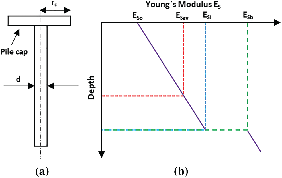
Figure 1: (a) Pile profile and (b) representation of modulus of elasticity of a simplified piled raft unit
The raft stiffness can be calculated using the formula given by Mayne et al. [57]. Also, single pile stiffness is calculated from the elastic theory and then multiplied by a group stiffness efficiency factor, which is estimated approximately from elastic solutions as discussed before. The proportion of the total applied load carried by the raft is:
where
The individual pile capacity for the present work is determined as per IS 2911 (Part 1: Section 2): 2010. The group capacity
Davis et al. [10] proposed a simplified load versus settlement curve to estimate the settlement of PRF (refer Fig. 2), the first part of this curve (from point O to point A) is used when the total applied load (
On the other hand, when the total applied load (
The reliability of a geotechnical structure is its ability to fulfill its design objectives for a given period under certain loading conditions. In other words, it is the probability that the structure does not reach the specified limit state for a specified period. For carrying out RA, it is necessary to define relationships between a set of input and output variables. Explicit relationship for RA was obtained from the analytical formulation given by Davis et al. [10] and Clancy et al. [11]. In the present work, the reliability of the PRF was performed based on serviceability limit state criterion; and the method adopted for RA is the First Order Reliability Method (FORM). A brief description of the said method is described below.
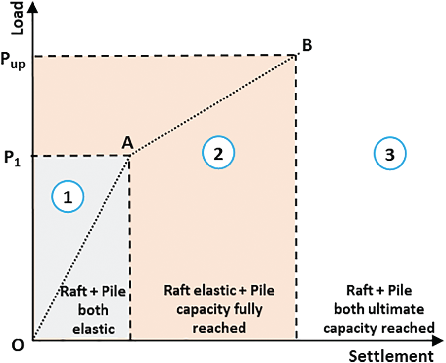
Figure 2: Load settlement curve for a simple PRF [10]
FORM is based upon the first few terms of Taylor’s series expansion [58]. This method is useful for estimating the mean value and variance of the performance function. FORM is often referred to as the first-order second-order method (FOSM).
Let the demand (expected loadings) of an engineering system is
This limit state function divides a region between the safe and unsafe condition. The probability of failure may be expressed as:
Using the above equations, the reliability index,
where
where
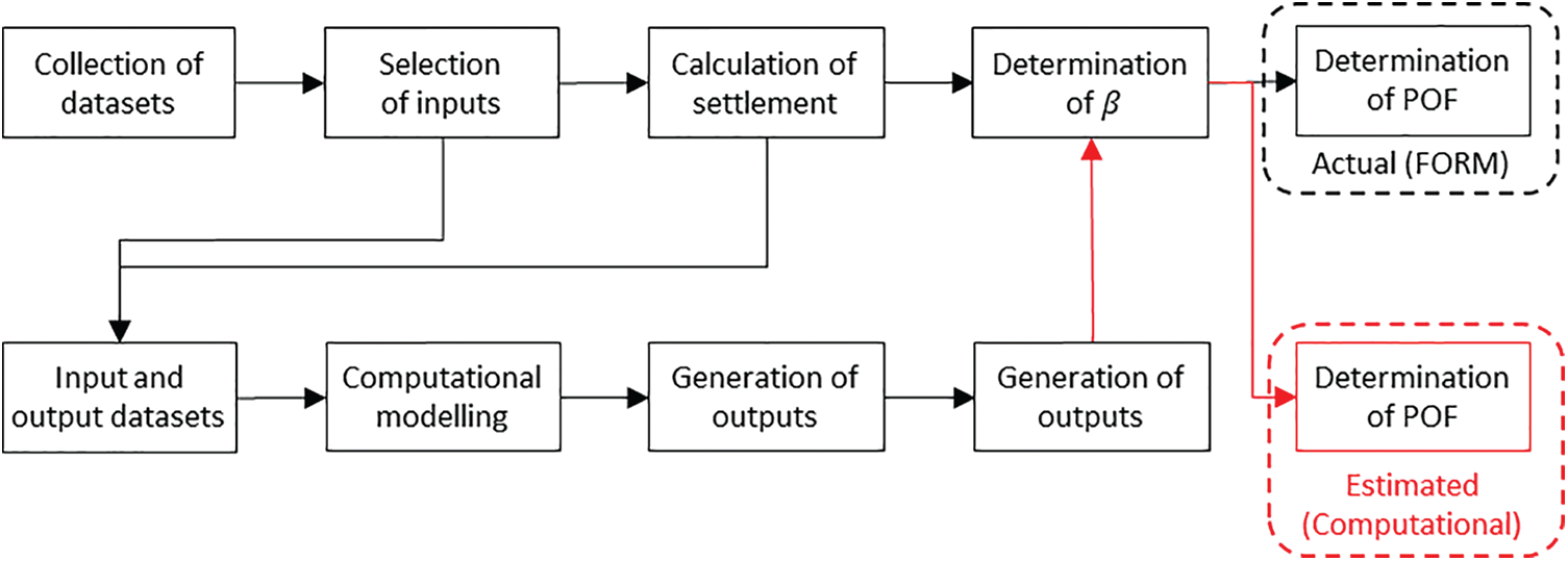
Figure 3: A process diagram of RA through FORM and computational modelling
2.4 Theoretical Background of the Employed Algorithms
In this sub-section, short descriptions of different soft computing techniques are presented. Begin with presenting the methodologies of ANN, GP, and MARS used in this study, which is followed by discussing the working principle of EO and PSO. Finally, the hybridization process of ANN-based hybrid models, i.e., ANN-EO and ANN-PSO are presented.
2.4.1 Artificial Neural Network (ANN)
ANN is a bio-inspired computing model made up of hundreds of individual units (artificial neurons) attached to coefficients (weights) that establish the neural structure. A structure of ANN consists of an input layer, hidden layer, and output layer with one or more neurons in each layer. As they play a role in information processing, they are also called processing elements (PEs). Each PE has its output, weighted inputs, and transfer function. PE is basically an equation that strikes a balance between inputs and outputs. Since connection weights denote the system memory, ANNs are also referred to as connectionist models. ANN has become a popular mathematical instrument for various purposes, including function approximation and pattern recognition. Successful application of this ML algorithm can be found in the literature [22–24,26,27].
2.4.2 Genetic Programming (GP)
GP is a symbolic optimization technique that creates computer programs based on the principle of Darwinian natural selection [63–65]. It is an extension of genetic algorithms (GA). The method was originally proposed by Koza [66], which mimics the biological evolution of living organisms. In GP, initially, a random population of individuals is created to achieve high diversity. Note that, the creation of initial populations is a blind random search. Once the initial population is created, GP evaluates individuals, selects them for reproduction, and generates new individuals by mutation, crossover, and reproduction; and finally, it creates new generations in all iterations.
In GP, the evolutionary process (a combination of crossover, mutation, and reproduction) continues by evaluating the fitness of the new population and starts a new round of evolutionary process in the next iteration. The best program that appeared in any generation, the best-so-far solution, defines the output of the GP algorithm. Successful implementation of this regression technique can be found in the analysis of slope stability, liquefaction susceptibility, compressive strength of concrete, including other areas of civil engineering [63–65,67–75].
2.4.3 Multivariate Adaptive Regression Splines (MARS)
MARS, introduced by Friedman [76] is a non-parametric regression technique that is capable of modelling non-linear relationships between the independent and dependent variables. It uses series of piecewise linear segments having different gradients known as splines. Splines are the flexible linear lines that are linked with knots. MARS simplifies complex multivariate datasets to relatively simple and linear additive models. It uses recursive partitioning and spline fitting to handle both quantitative and categorical predictors.
In the first phase, i.e., forward phase, it selects only one input variable and placed the knots at random positions within the range of each predictor to define a pair of Basis functions (BFs). BFs is nothing but a spline. In each step, the knot and its corresponding pair of BFs are fitted to yield the maximum reduction in sum-of-squares residual error by adding new BFs until the minimum threshold value is reached. However, the addition of BFs yields a complex and over-fitted model which shows poor performance for the new dataset.
In order to improve the performance of the over-fitted model, MARS starts pruning of least performing BFs in the subsequent phase, i.e., deletion of BFs takes place in the phase. Generally, MARS removes one BF at a time and assesses the model based on the generalized-cross-validation (GCV) criterion [72,77]. This process continues until the lack-of-fit criterion is minimum. Finally, produced the optimum model with the optimum number of BFs.
2.4.4 Equilibrium Optimizer (EO)
EO is a recently developed meta-heuristic optimization algorithm [49], resourced from physics-based dynamic mass balance theory. It typically characterizes the interaction of search agents according to governing rules rooted in physical processes. The working principle of EO is similar to the other metaheuristics algorithms where the search operation is performed using a set of candidate solutions. During the search, the candidate solutions update their concentration with respect to the best solution obtained till that point, to finally arrive at the equilibrium state, which provides the optimal result. These candidate solutions are called concentration vectors (CVs) given by:
where
where
where
where
The iteration rate
where
2.4.5 Particle Swarm Optimization (PSO)
PSO is a population-based meta-heuristic algorithm introduced by Kennedy et al. [78] as a member of the swarm-based community. The PSO algorithm has mainly been inspired by fish schools or bird flocks, whose main purpose is to find globally optimal solutions in a multidimensional space. It starts with the initialization of particle positions and random velocities. To find the best position in the multidimensional space, each particle then attempts to update its position based on its velocity, as well as the personal best position (best position reached by a single particle) and global best position (best position reached by individual particles). The position of each particle is updated based on its personal best position and the direction of the global best position. Meanwhile, particle velocity is updated according to the difference between its personal and global best positions. The particles then use a combination of exploration and exploitation to converge around the optimal solution. The velocity and position of a particle in each iteration is given by:
where
where
2.4.6 Hybridization of ANN-Based Meta-Heuristic Models
In engineering applications, many studies have been performed to enhance the performance of traditional ML algorithms by implementing meta-heuristic OAs, such as PSO, GA, etc. Due to the weakness of traditional ML algorithms, such as ANN, in finding the exact global minimum, ANN may produce undesirable results [24,27]. In addition, ANN is more likely to be caught up in local minima. Therefore, implementing meta-heuristic OAs can solve the problem by optimizing the learning parameters (weights and biases) based on error criteria.
In this study, two meta-heuristic OAs, namely EO and PSO are used to optimize the weights and biases of conventional ANN. The learning parameters of ANN include input to hidden weights, hidden biases, hidden to output weights, and output biases. A model with
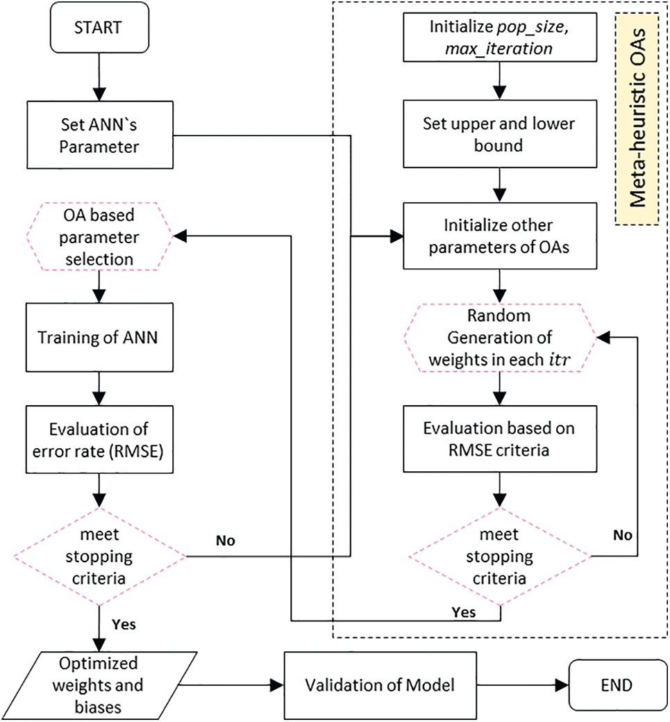
Figure 4: Flow chart showing the steps in developing ANN-based hybrid models
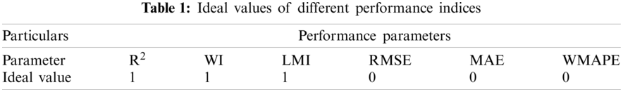
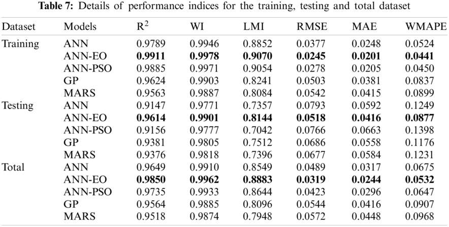
To assess the performance of the developed models, six widely used performance indices, namely determination coefficient (R2), Willmott’s Index of agreement (WI), Legates & McCabe’s Index (LMI), root mean square error (RMSE), mean absolute error (MAE), and weighted mean absolute error (WMAPE) were determined and assessed in detail. The details of these indices can be found in the literature [16,79–86]; however, for convenience, the mathematical expressions are given below. In addition, for a perfect predictive model, the ideal values of these indices are given in Tab. 1.
where
3 Description of the Study Site and Collected Dataset
The site under consideration is located near the Harohar River (lat. 25° 12′49.5″ N, long. 86° 04′13.9″ E) was selected as the study area. A 2.5 m wide approach road was planned to be built towards a bridge over the river Harohar. Since the proposed level of the approach road was higher than the existing ground level aligning with the river; the soil was dumped to raise the existing ground level up to the level of the approach road. But, after filling of soil material, bearing capacity failure was observed for the existing ground level. Later, a cantilever retaining wall was proposed to be constructed at the site in order to support the soil standing up to the level of the approach road. The details of the cantilever retaining wall are shown in Fig. 5. It is observed that the underlying soil has poor properties in terms of cohesion (
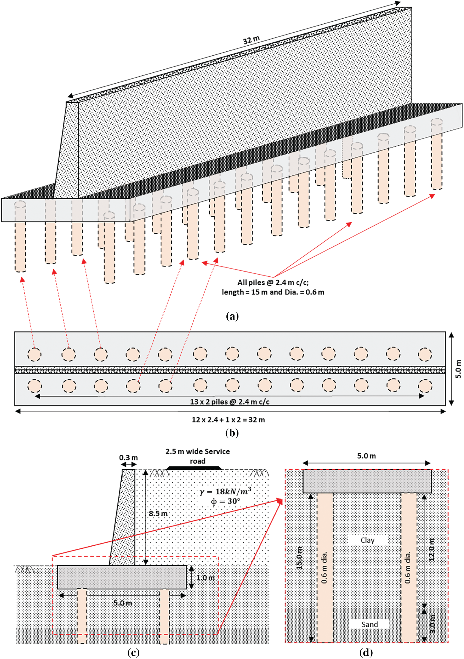
Figure 5: Schematic details of the proposed PRS: (a) Cantilever retaining wall with pile arrangement; (b) top view of PRS; and (c, d) sectional view of PRS
To obtain information about the sub-soil conditions, 7 boreholes of 15 m each were dug and soil samples with a diameter of 38 mm were collected by the method of SPT. The soil samples were collected at an interval of 1.5 m depth. After the geotechnical investigation, necessary soil tests were carried out and the information extracted from the tests include
In this section, the analysis of the proposed PRF, which is supposed to carry the load from a cantilever retaining wall is presented. Fig. 5 shows the details of PRF, including the details of each pile and sub-soil properties. As can be seen, the proposed PRF consists of 26 piles, a 1 m thick raft, and an 8.5 m high cantilever retaining wall with a 5 m wide base. All piles are 15 m long and 0.6 m in diameter. The spacing between the piles is 2.4 m in both directions. The overall height of the retaining wall including the raft is 9.5 m. The width of the stem of the retaining wall at the top is 0.30 m, and it increased to 0.6 m at the base giving a clearance of 2.2 m on each side of the raft. The cantilever retaining wall was designed to construct the approach road as shown in Fig. 5c.
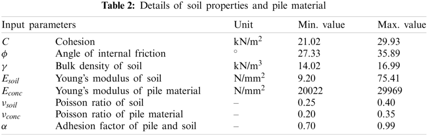
Different soil properties, such as
In the first step, the incoming load and the moment on the PRF were calculated. The retaining wall is shown in Fig. 5c, was analyzed for the total height of the backfill material with soil properties
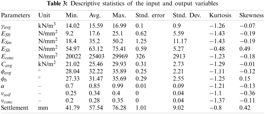
In the subsequent step, RA of PRF was performed considering the most important influencing parameters, i.e.,
It is pertinent to mention here that, the aforementioned parameters (
5 Data Processing and Analysis
The most crucial step for any type of problem in the field of soft computing techniques, such as ANN techniques, is considered to be the normalization of data. This is a pre-processing phase. In the present study, 80% of the total dataset, i.e., the training dataset was used to construct the models, while the balance 20% dataset (testing dataset) was used to validate the developed models. Before the training and testing bifurcation, the total dataset was normalized in the range of 0 to 1 using the expression given by:
where
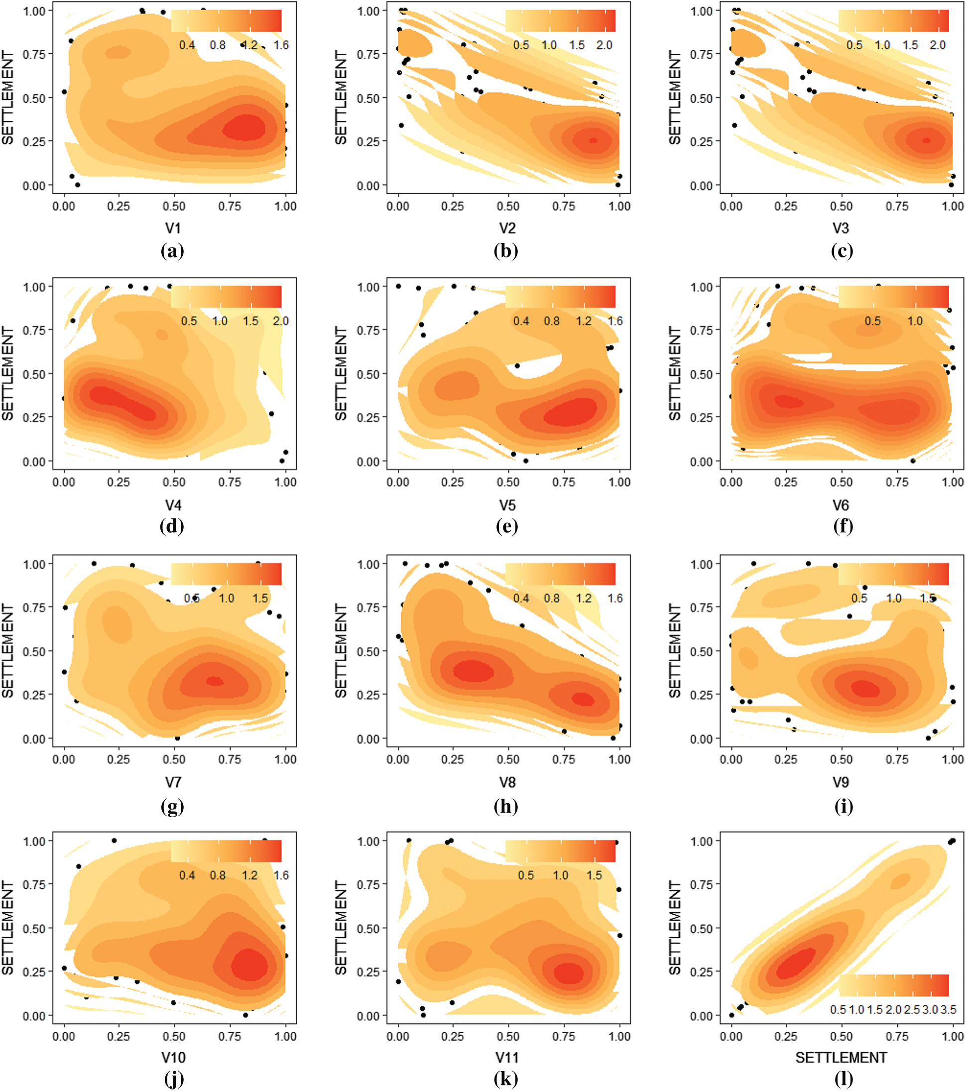
Figure 6: (a–l)—Scatter density plot between input and output variables (V1 to V11 represent input variable from 1 to 11)
6.1 Configuration of Developed Models
To determine the structure of the proposed ANN-based hybrid models, it is necessary to select the optimum number of hidden neurons for developing robust models. In the present study, the number of hidden neurons varying from 1 to 15 was examined for conventional ANN. In addition, the log-sigmoid and tan-sigmoid were used as the activation function. Following the trial-and-error approach, the most appropriate number of hidden neurons was obtained as 10 and the tan-sigmoid activation function was more appropriate for ANN-EO and ANN-PSO models. The EO and PSO optimized ANN includes 11 neurons in the input layer, 10 neurons in the hidden layer, and 1 neuron in the output layer (a structure of hybrid ANN model is presented in Fig. 7). The configuration of the proposed hybrid models including the details of population/particle size, the maximum number of iterations, upper and lower bounds, etc., are indicated in Tab. 4 along with the convergence behavior in Fig. 8.
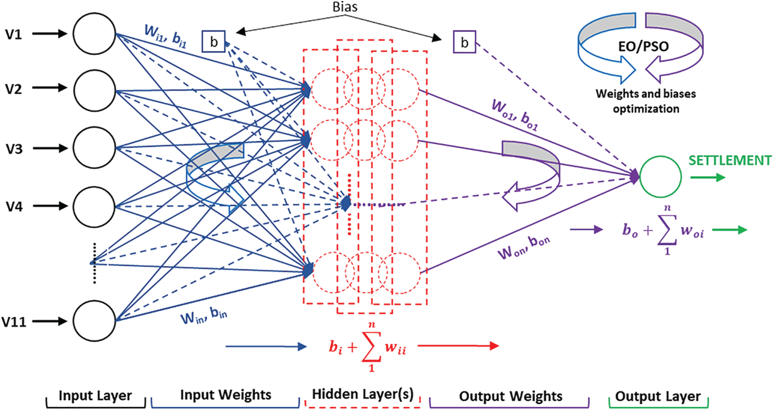
Figure 7: A structure of the developed hybrid ANN model
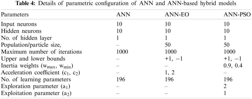
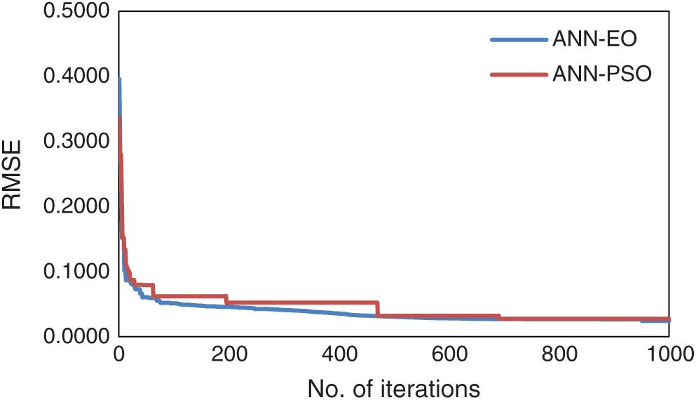
Figure 8: Convergence behavior of ANN-EO and ANN-PSO models
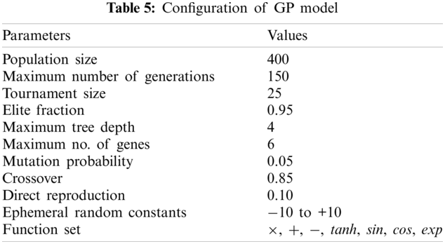
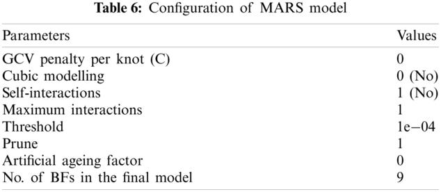
Opposite to the ANN-based models, the parameters of GP and MARS were also designed following the trial-and-error approach. Note that, for constructing an optimum model, the parameters of GP and MARS should be selected suitably. In GP, the parameters are population size, generation number, tournament size, elite fraction, tree depth, number of genes, mutation probability, crossover probability, reproduction probability, etc., while in MARS, number of BFs, GCV per knot, self-interaction, pruning, and aging factor are the most important parameters. It may also be noted that inappropriate values of such parameters increase the complexity of the prediction model, which in turn exhibits poor performance. Tabs. 5 and 6 list the details of GP and MARS parameters obtained through a trial-and-error approach. The following sub-section describes the outcomes of the developed ANN-based models including the GP and MARS in estimating the settlement of PRF, followed by the results of RA and POF.
6.2 Outcomes of the Developed Models
The prediction outcomes of the developed models in predicting the settlement of PRF are presented in Figs. 9 and 10 for the training dataset, and Figs. 11 and 12 for the testing dataset. Herein, the model performance when it was used to predict the settlement of PRF is reported first. It is noted that model performance with the training dataset was employed to express the goodness of fit of the developed models through the performance parameters, details of which are presented in Tab. 7. Based on the experimental results with the R2 and RMSE criteria, it can be seen the R2 values of the developed models lies in the range of 0.9563 to 0.9911 (training stage), while the values of RMSE lies in the range of 0.245 to 0.0542 (training stage). These results clearly demonstrate that the developed models obtained higher prediction performance in estimating the settlement of PRF. In addition, the values of MAE and WI in the training stage were obtained in the range of 0.201 to 0.0381 and 0.9887 to 9978, respectively, which also satisfies higher prediction accuracy. Tab. 7 also represents the outcomes of the developed models for the testing and total dataset. As can be seen, the values of R2 are higher than 0.90 in the training, testing, and total phases, which indicates that the developed models obtained a good fit to the actual dataset. Among the developed models, the proposed ANN-EO and ANN-PSO models attainted higher prediction accuracy with R2 = 0.9911 and R2 = 0.9885 in the training stage, and, R2 = 0.9614 and R2 = 0.9156 in the testing stage. Overall, the GP and MARS attained the lowest prediction accuracy with R2 = 0.9564 and R2 = 0.9518, respectively.
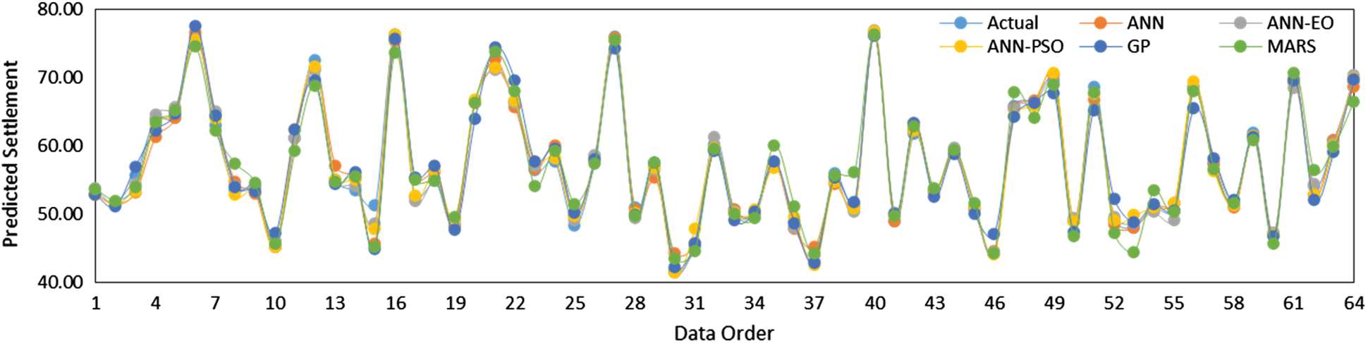
Figure 9: Actual vs. predicted settlement values for the training dataset
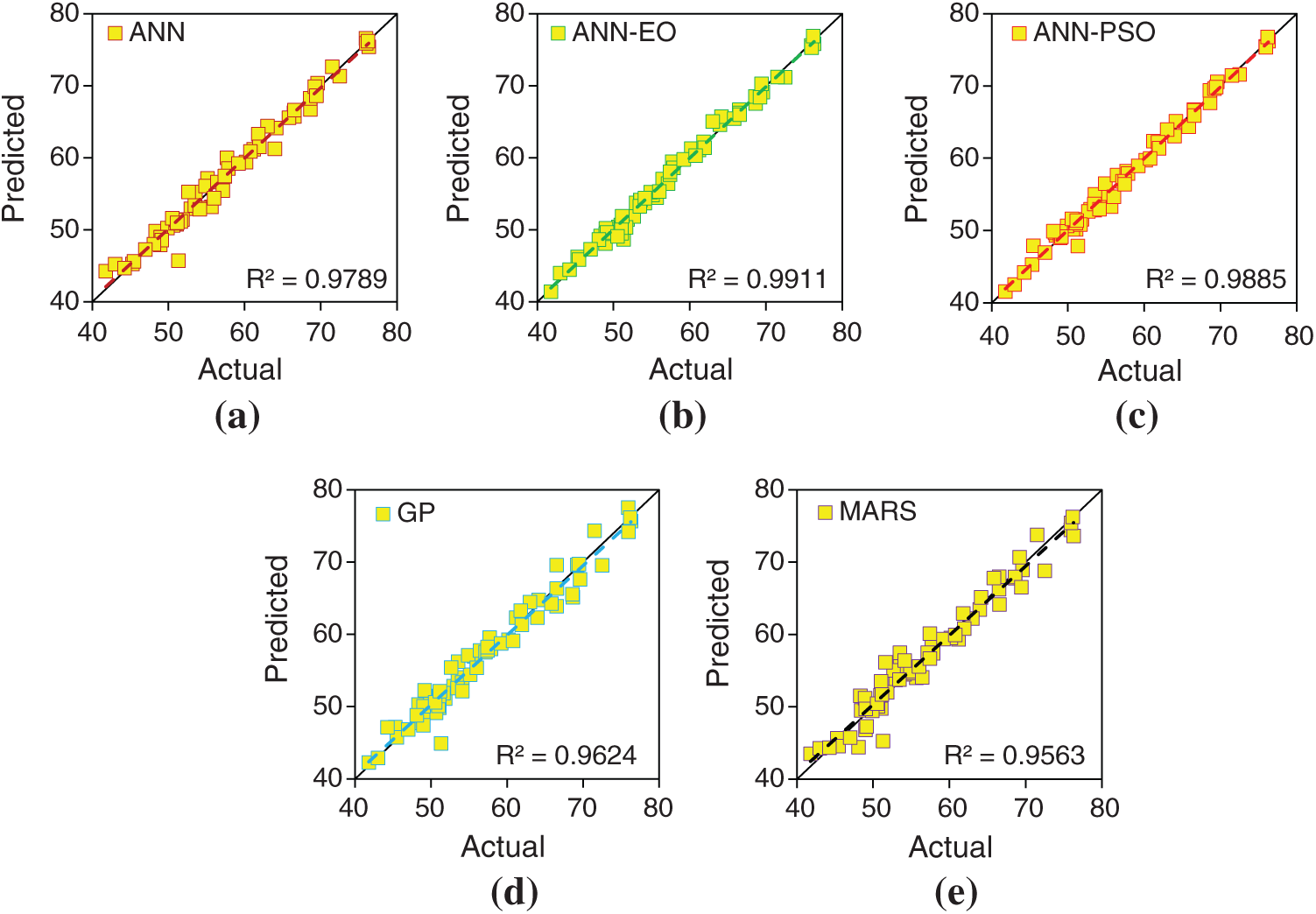
Figure 10: (a–e)—Illustrations of actual and predicted values for the training dataset
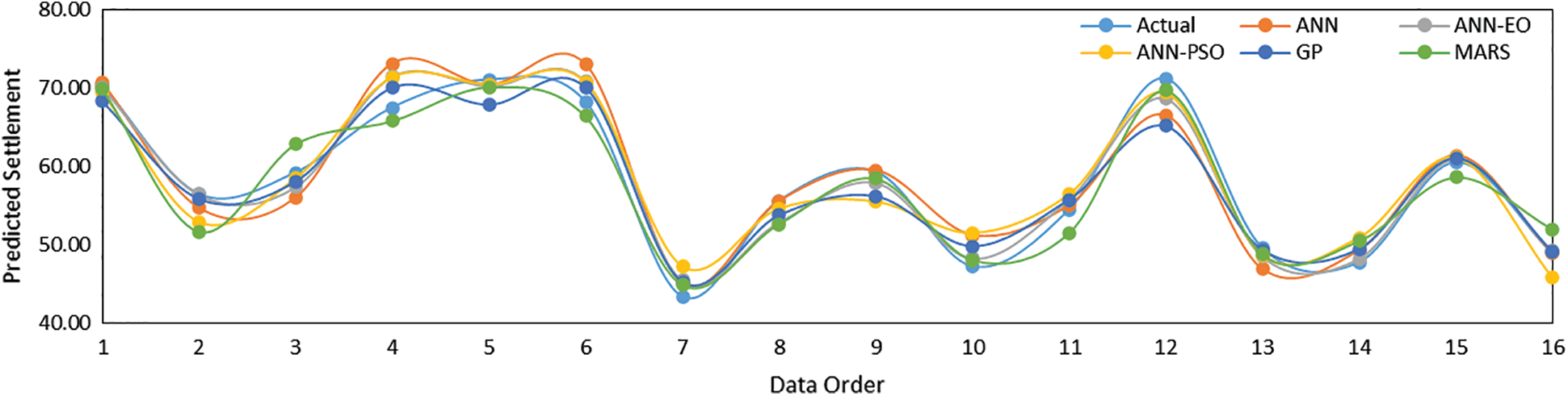
Figure 11: Actual vs. predicted settlement values for the testing dataset
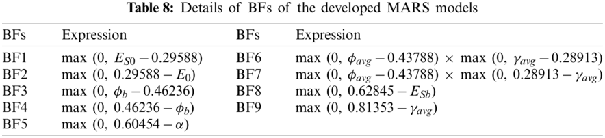
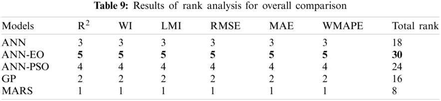
The final GP and MARS models are presented in Eqs. (48) and (49), respectively. The GP expression given in Eq. (48) is a combination of 6 genes and a bias term, while the MARS model consists of 9 BFs. The details of BFs are presented in Tab. 8. It may be noted that, although the said models unable to attain the highest prediction accuracy; however, considering the experimental results (R2, RMSE, and MAE criteria), the developed predictive expressions can readily be used to predict the settlement of PRF. The overall performance of the proposed ANN-EO model was also assessed through rank analysis [79–81], the results of which are presented in Tab. 9. As can be seen, the proposed ANN-EO model attained the highest total rank of 30 and outperformed the other models by far. The MARS and GP are the worst-performing models in this case.
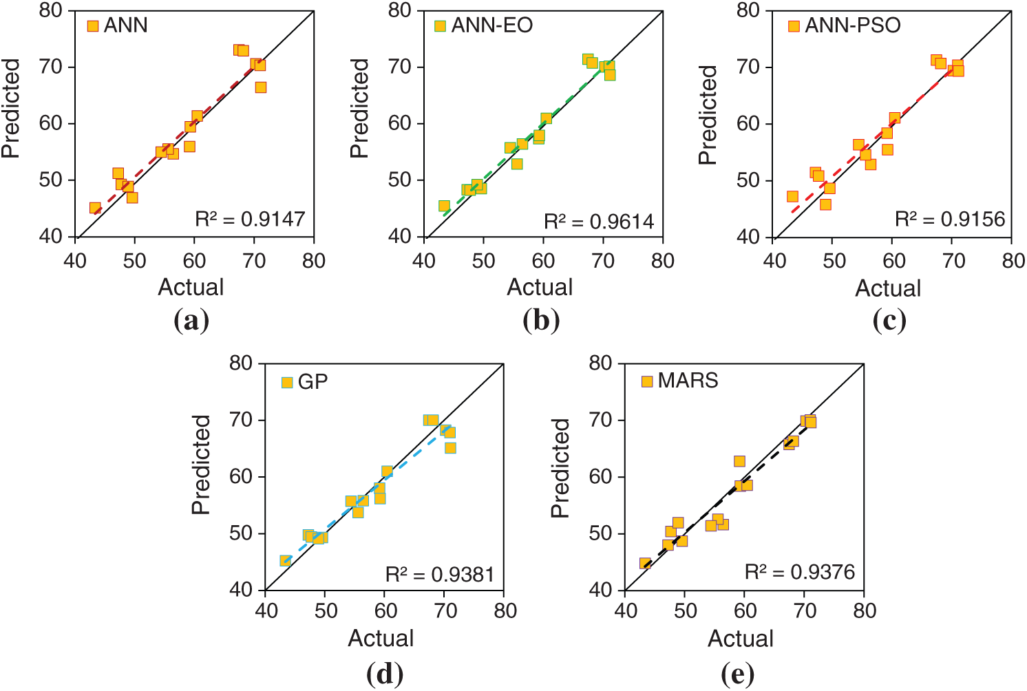
Figure 12: (a–e)—Illustrations of actual and predicted values for the testing dataset
Tab. 10 reports the values of
a) Determination of mean settlement value (
b) Determination of standard deviation of settlement values (
c) Determination of mean and standard deviation of permissible settlement value, i.e.,
d) Determination of
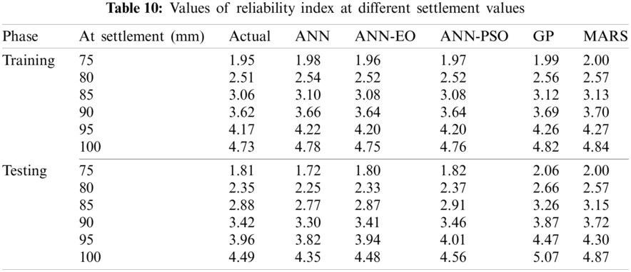
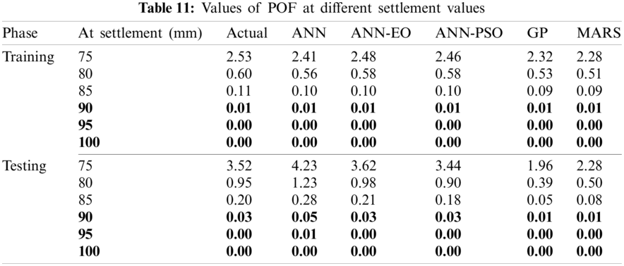
Subsequently, the POF of the proposed PRF was determined using the expression given in Eq. (27), separately for training and testing datasets, the details of which are reported in Tab. 11. Note that, the values of POF reported herein are in percentage term. From the results presented in Tabs. 10 and 11, it is clearly observed that the proposed ANN-EO and ANN-PSO able to estimate the risk associated with the proposed PRF in terms of
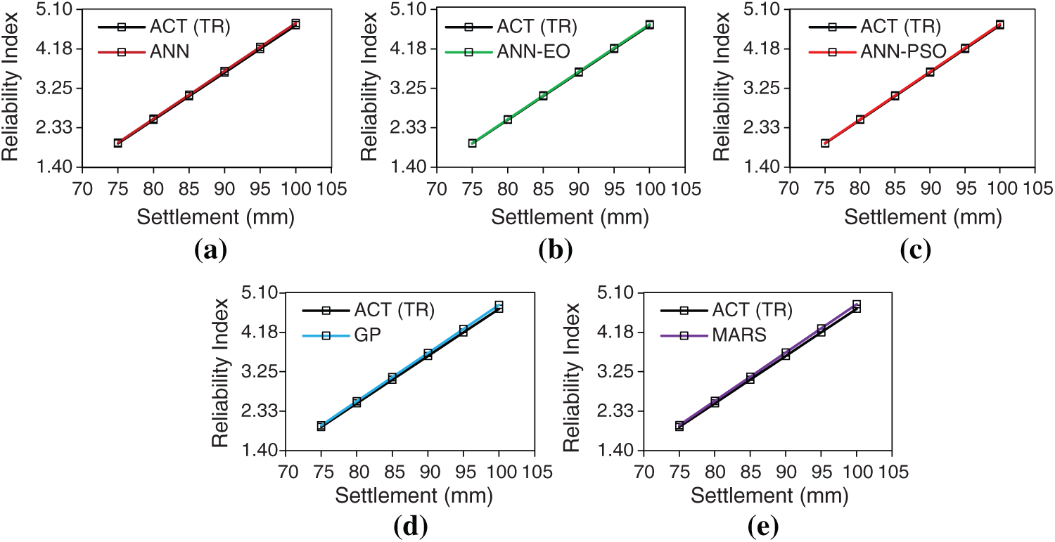
Figure 13: (a–e)—Settlement vs. Reliability Index plot for the training dataset (model wise)
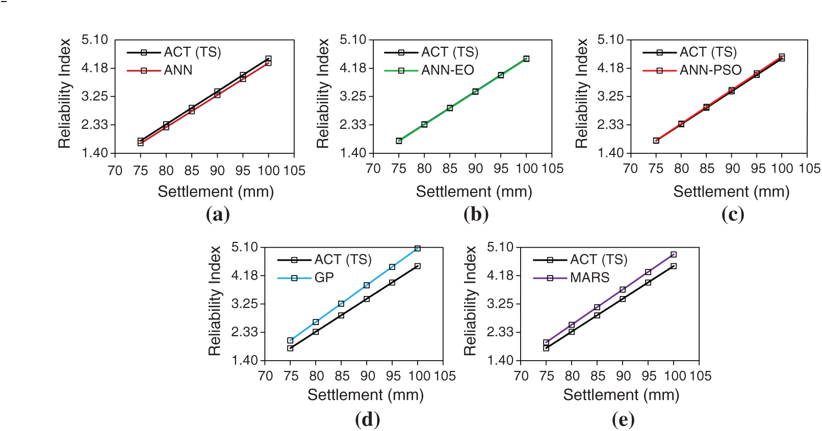
Figure 14: (a–e)—Settlement vs. Reliability Index plot for the testing dataset (model wise)
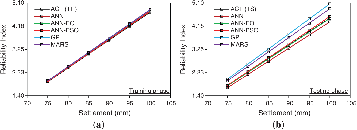
Figure 15: (a–b)—Settlement vs. Reliability Index plot (all models together)
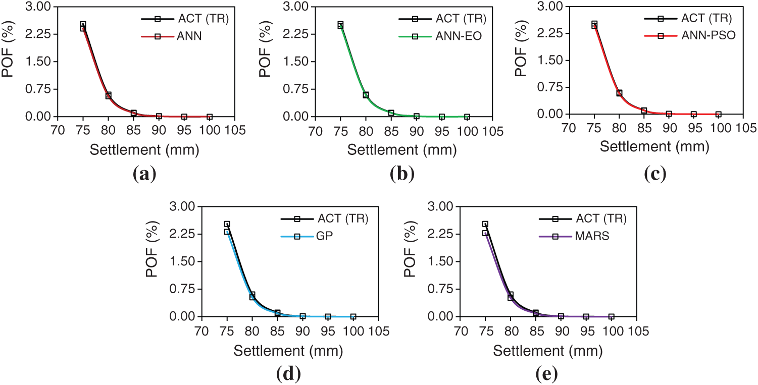
Figure 16: (a–e)—Settlement vs. Probability of failure plot for the testing dataset (model wise)
As mentioned earlier, the proposed PRF consists of 26 piles and all piles are 15 m long. The top 12 m is embedded in the clayey layer while the bottom 3 m is resting in sandy soil. The present problem, the settlement of raft foundation (without piles) was estimated as 113.68 mm, which exceeds the permissible value of 100 mm as per IS 1904–1986. Note that, if the estimated settlement of raft foundation is greater than the permissible limit, it would be necessary to introduce piles as a measure of settlement reducer. Therefore, to restrict the settlement within the permissible value, a combination of raft and piles, i.e., PRF was selected as the foundation type. For the same conditions, the revised settlement was calculted as 66.08 mm only. However, to investigate the failure probability of the proposed PRF in a more comprehensive manner, values of
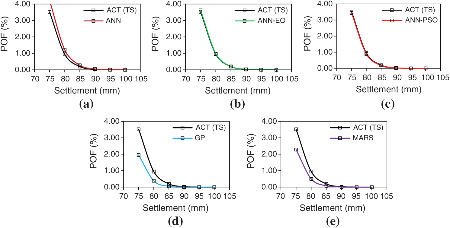
Figure 17: (a–e)—Settlement vs. Probability of failure plot for the testing dataset (model wise)
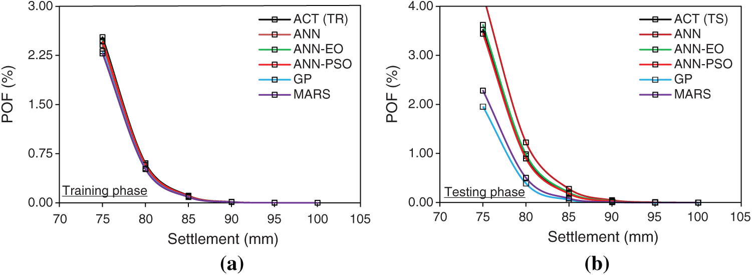
Figure 18: (a–b)—Settlement vs. Probability of failure plot (all models together)
This study presents a high-performance soft computing technique to perform the RA of PRF. The proposed model is a combination of the classical ANN and EO, i.e., ANN-EO. Initially, the ANN-EO was employed to construct a prediction model for estimating the settlement of PRF from a set of 11 influencing factors. Later, the ANN-EO along with other developed models (ANN, MARS, GP, and ANN-PSO) were used to investigate the risk associated with the PRF in terms of POF. The failure probability of PRF with cantilever retailing wall arrangement was investigated for a set of settlement values ranging from 75 to 100 mm. This was done to investigate the inter-relationship between the settlement and POF for the proposed PRF. The theoretical analysis suggested that the proposed PRF attained almost negligible failure probability (in the range of 0.01% to 0.03%) at 90 mm or more permissible settlement value. Therefore, the proposed PRF could be considered safe against settlement failure at a designed permissible settlement value of 90 mm.
All the proposed models demonstrate higher prediction results to the actual POF in the training phase, while the proposed hybrid ANN-EO model attained the most desired prediction value with R2 = 0.9911, RMSE = 0.0245, and MAE = 0.0201 in the training stage, and R2 = 0.9614, RMSE = 0.0518, and MAE = 0.0416 in the testing phase. These outcomes are significantly better than those obtained from ANN-PSO, including the traditional ANN, GP, and MARS used to estimate the failure probability of the proposed PRF. The computational cost of the proposed ANN-EO and ANN-PSO was recorded as 421.860941 s and 429.964295 s, respectively, using MATLAB environment with MATLAB 2015a, i7-4790 CPU @ 3.60 GHz, 8 GB RAM. The main advantages of the proposed ANN-EO model include higher prediction accuracy, ease of implementation using the existing dataset, and high generalization capability. The future direction of this study may include a) integration of ANN and other meta-heuristic OAs and a detailed comparison of ANN-EO with other hybrid ANN models, b) use of deep learning models and construction of hybrid models of deep learning models and meta-heuristic OAs, c) selection of input parameters using feature selection techniques, d) implementation of dimension reduction procedure and inter-quartile technique to handle noise in the dataset, and e) reduction of computational costs using an enhanced version of OAs. In addition, implementation of other reliability-based analyses to compare the results of FORM and the developed models in detail. Nevertheless, the concept proposed in this study can be used to perform RA of other civil engineering structures; however, the existing database should be prepared before the estimation of the reliability index and its corresponding POF. Based on these facts, the proposed ANN-EO can be used as a promising alternative to estimate the POF of PRF, including many other civil engineering structures. As per the authors’ knowledge, the implementation of hybrid ANN models, specifically ANN-EO for performing the reliability analysis of PRF would significantly contribute to the knowledge pool of reliability studies related to PRF due to the fact that the literature on reliability analysis of PRS is relatively scarce.
Author's Contributions: A. Bardhan: Main author, conceptualization, overall analysis, development of AI models, detailing, and manuscript finalization; P. Manna: Theoretical analysis; V. Kumar: Referencing; A. Burman: Overall review; B. Žlender: Overall review; P. Samui: Overall review.
Funding Statement: The authors received no specific funding for this study.
Conflicts of Interest: The authors declare that they have no conflicts of interest to report regarding the present study.
1. Al-Kinani, A. S. H. R. A. F., Reddy, D. E. S. (2014). Design of the piled raft foundations for load settlement behavior using a multiphase model. International Journal of Scientific Enginh. keering and Technology, 3, 4766–4776. http://ijsetr.com/uploads/514326IJSETR2097-842.pdf. [Google Scholar]
2. Ghorbani, A., Firouzi Niavol, M. (2017). Evaluation of induced settlements of piled rafts in the coupled static-dynamic loads using neural networks and evolutionary polynomial regression. Applied Computational Intelligence and Soft Computing, 2017(2), 1–23. DOI 10.1155/2017/7487438. [Google Scholar] [CrossRef]
3. Niandou, H., Breysse, D. (2007). Reliability analysis of a piled raft accounting for soil horizontal variability. Computers and Geotechnics, 34(2), 71–80. DOI 10.1016/j.compgeo.2006.09.006. [Google Scholar] [CrossRef]
4. Griffiths, D. V., Clancy, P., Randolph, M. F. (1991). Piled raft foundation analysis by finite elements. International Conference on Computer Methods and Advances in Geomechanics, vol. 7, pp. 1153–1157. Cairns, Australia. [Google Scholar]
5. Horikoshi, K., Randolph, M. F. (1998). A contribution to optimum design of piled rafts. Geotechnique, 48(3), 301–317. DOI 10.1680/geot.1998.48.3.301. [Google Scholar] [CrossRef]
6. Poulos, H. G. (1994). An approximate numerical analysis of pile-raft interaction. International Journal for Numerical and Analytical Methods in Geomechanics, 18(2), 73–92. DOI 10.1002/(ISSN)1096-9853. [Google Scholar] [CrossRef]
7. Brzakała, W., Puła, W. (1996). A probabilistic analysis of foundation settlements. Computers and Geotechnics, 18(4), 291–309. DOI 10.1016/0266-352X(95)00033-7. [Google Scholar] [CrossRef]
8. Russo, G. (1998). Numerical analysis of piled rafts. International Journal for Numerical and Analytical Methods in Geomechanics, 22(6), 477–493. DOI 10.1002/(ISSN)1096-9853. [Google Scholar] [CrossRef]
9. Kim, K. N., Lee, S. H., Kim, K. S., Chung, C. K., Kim, M. M. et al. (2001). Optimal pile arrangement for minimizing differential settlements in piled raft foundations. Computers and Geotechnics, 28(4), 235–253. DOI 10.1016/S0266-352X(01)00002-7. [Google Scholar] [CrossRef]
10. Davis, E. H., Poulos, H. G. (1972). The analysis of piled raft systems. Australian Geomech Journal G2, 21–27. [Google Scholar]
11. Clancy, P., Randolph, M. F. (1996). Simple design tools for piled raft foundations. Geotechnique, 46(2), 313–328. DOI 10.1680/geot.1996.46.2.313. [Google Scholar] [CrossRef]
12. Kumar, M., Samui, P. (2019). Reliability analysis of pile foundation using ELM and MARS. Geotechnical and Geological Engineering, 37(4), 3447–3457. DOI 10.1007/s10706-018-00777-x. [Google Scholar] [CrossRef]
13. Duncan, J. M. (2000). Factors of safety and reliability in geotechnical engineering. Journal of Geotechnical and Geoenvironmental Engineering, 126(4), 307–316. DOI 10.1061/(ASCE)1090-0241(2000)126:4(307). [Google Scholar] [CrossRef]
14. Kumar, M., Samui, P. (2020). Reliability analysis of settlement of pile group in clay using LSSVM, GMDH. GPR Geotechnical and Geological Engineering, 38(6), 6717–6730. DOI 10.1007/s10706-020-01464-6. [Google Scholar] [CrossRef]
15. Kumar, M., Samui, P., Kumar, D., Zhang, W. (2021). Reliability analysis of settlement of pile group. Innovative Infrastructure Solutions, 6(1), 1–17. [Google Scholar]
16. Kumar, M., Bardhan, A., Samui, P., Hu, J. W., Kaloop, R. et al. (2021). Reliability analysis of pile foundation using soft computing techniques: A comparative study. Processes, 9(3), 486. DOI 10.3390/pr9030486. [Google Scholar] [CrossRef]
17. Kumar, R., Samui, P., Kumari, S., Roy, S. S. (2021). Determination of reliability index of cantilever retaining wall by RVM, MPMR and MARS. International Journal of Advanced Intelligence Paradigms, 18(3), 316–336. DOI 10.1504/IJAIP.2021.113325. [Google Scholar] [CrossRef]
18. Kumar, R., Samui, P., Kumari, S., Dalkilic, Y. H. (2021). Reliability analysis of circular footing by using GP and MPMR. International Journal of Applied Metaheuristic Computing, 12(1), 1–19. DOI 10.4018/IJAMC. [Google Scholar] [CrossRef]
19. Ray, R., Kumar, D., Samui, P., Roy, L. B., Goh, A. T. C. et al. (2021). Application of soft computing techniques for shallow foundation reliability in geotechnical engineering. Geoscience Frontiers, 12(1), 375–383. DOI 10.1016/j.gsf.2020.05.003. [Google Scholar] [CrossRef]
20. Tawfik, M. E., Bishay, P. L., Sadek, E. A. (2018). Neural network-based second order reliability method (NNBSORM) for laminated composite plates in free vibration. Computer Modeling in Engineering & Sciences, 115(1), 105–129. DOI 10.3970/cmes.2018.115.105. [Google Scholar] [CrossRef]
21. Kerh, T., Lai, J. S., Gunaratnam, D., Saunders, R. (2008). Evaluation of seismic design values in the Taiwan building code by using artificial neural network. Computer Modeling in Engineering & Sciences, 26(1), 1. https://www.techscience.com/CMES/v26n1/25101. [Google Scholar]
22. Karaci, A., Yaprak, H., Ozkaraca, O., Demir, I., Simsek, O. (2019). Estimating the properties of ground-waste-brick mortars using DNN and ANN. Computer Modeling in Engineering & Sciences, 118(1), 207–228. DOI 10.31614/cmes.2019.04216. [Google Scholar] [CrossRef]
23. Roy, B., Singh, M. P. (2020). An empirical-based rainfall-runoff modelling using optimization technique. International Journal of River Basin Management, 18(1), 49–67. DOI 10.1080/15715124.2019.1680557. [Google Scholar] [CrossRef]
24. Koopialipoor, M., Fallah, A., Armaghani, D. J., Azizi, A., Mohamad, E. T. (2019). Three hybrid intelligent models in estimating flyrock distance resulting from blasting. Engineering with Computers, 35(1), 243–256. DOI 10.1007/s00366-018-0596-4. [Google Scholar] [CrossRef]
25. Livingstone, D. J., Manallack, D. T., Tetko, I. V. (1996). Data modeling with neural networks—An answer to the maiden’s prayer. Journal of Computer-Aided Molecular Design, 11(2), 135–142. DOI 10.1023/A:1008074223811. [Google Scholar] [CrossRef]
26. Mishra, M., Srivastava, M. (2014). A view of artificial neural network. 2014 International Conference on Advances in Engineering & Technology Research, pp. 1–3. Unnao, India, IEEE. DOI 10.1109/ICAETR.2014.7012785. [Google Scholar] [CrossRef]
27. Liou, S. W., Wang, C. M., Huang, Y. F. (2009). Integrative discovery of multifaceted sequence patterns by frame-relayed search and hybrid PSO-ANN. Journal of Universal Computer Science, 15(4), 742–764. DOI 10.3217/jucs-015-04-0742. [Google Scholar] [CrossRef]
28. Moayedi, H., Moatamediyan, A., Nguyen, H., Bui, X. N., Bui, D. T. et al. (2020). Prediction of ultimate bearing capacity through various novel evolutionary and neural network models. Engineering with Computers, 36(2), 671–687. DOI 10.1007/s00366-019-00723-2. [Google Scholar] [CrossRef]
29. Le, L. T., Nguyen, H., Dou, J., Zhou, J. (2019). A comparative study of PSO-ANN, GA-ANN, ICA-ANN, and ABC-ANN in estimating the heating load of buildings’ energy efficiency for smart city planning. Applied Sciences, 9(13), 2630. DOI 10.3390/app9132630. [Google Scholar] [CrossRef]
30. Bui, D. T., Nhu, V. H., Hoang, N. D. (2018). Prediction of soil compression coefficient for urban housing project using novel integration machine learning approach of swarm intelligence and multi-layer perceptron neural network. Advanced Engineering Informatics, 38, 593–604. DOI 10.1016/j.aei.2018.09.005. [Google Scholar] [CrossRef]
31. Fattahi, H., Bayatzadehfard, Z. (2018). Forecasting surface settlement caused by shield tunneling using ANN-BBO model and ANFIS based on clustering methods. Journal of Engineering Geology, 12, 55. DOI 10.18869/acadpub.jeg.12.5.55. [Google Scholar] [CrossRef]
32. Nguyen, M. D., Pham, B. T., Ho, L. S., Ly, H. B., Le, T. T. et al. (2020). Soft-computing techniques for prediction of soils consolidation coefficient. Catena, 195, 104802. DOI 10.1016/j.catena.2020.104802. [Google Scholar] [CrossRef]
33. Akbal, B. (2018). GSA-ANN and DEA-ANN methods to prevent underground cable line faults. International Journal of Computer and Electrical Engineering, 10(2), 85–93. DOI 10.17706/IJCEE.2018.10.2.85-93. [Google Scholar] [CrossRef]
34. Rao, A. N., Vijayapriya, P. (2019). A robust neural network model for monitoring online voltage stability. International Journal of Computers and Applications, 41, 1–10. DOI 10.1080/1206212X.2019.1666224. [Google Scholar] [CrossRef]
35. Yang, Z. C., Sun, W. C. (2013). A set-based method for structural eigenvalue analysis using Kriging model and PSO algorithm. Computer Modeling in Engineering & Sciences, 92(2), 193–212. DOI 10.3970/cmes.2013.092.193. [Google Scholar] [CrossRef]
36. Hou, G., Xu, Z., Liu, X., Jin, C. (2019). Improved particle swarm optimization for selection of shield tunneling parameter values. Computer Modeling in Engineering & Sciences, 118(2), 317–337. DOI 10.31614/cmes.2019.04693. [Google Scholar] [CrossRef]
37. Sunil, N., Ganesan, R., Sankaragomathi, B. (2019). Analysis of OSA syndrome from PPG signal using CART-PSO classifier with time domain and frequency domain features. Computer Modeling in Engineering & Sciences, 118(2), 351–375. DOI 10.31614/cmes.2018.04484. [Google Scholar] [CrossRef]
38. Hasanipanah, M., Shahnazar, A., Amnieh, H. B., Armaghani, D. J. (2017). Prediction of air-overpressure caused by mine blasting using a new hybrid PSO-SVR model. Engineering with Computers, 33(1), 23–31. DOI 10.1007/s00366-016-0453-2. [Google Scholar] [CrossRef]
39. Sujith, M., Padma, S. (2020). Implementation of PSOANN optimized PI control algorithm for shunt active filter. Computer Modeling in Engineering & Sciences, 122(3), 863–888. DOI 10.32604/cmes.2020.08908. [Google Scholar] [CrossRef]
40. Li, G., Kumar, D., Samui, P., Nikafshan Rad, H., Roy, B. et al. (2020). Developing a new computational intelligence approach for approximating the blast-induced ground vibration. Applied Sciences, 10(2), 434. DOI 10.3390/app10020434. [Google Scholar] [CrossRef]
41. Kaloop, M. R., Kumar, D., Zarzoura, F., Roy, B., Hu, J. W. (2020). A wavelet-particle swarm optimization-extreme learning machine hybrid modeling for significant wave height prediction. Ocean Engineering, 213(11), 107777. DOI 10.1016/j.oceaneng.2020.107777. [Google Scholar] [CrossRef]
42. Ly, H. B., Pham, B. T., Le, L. M., Le, T. T., Le, V. M. et al. (2021). Estimation of axial load-carrying capacity of concrete-filled steel tubes using surrogate models. Neural Computing and Applications, 33(8), 3437–3458. DOI 10.1007/s00521-020-05214-w. [Google Scholar] [CrossRef]
43. Hajihassani, M., Armaghani, D. J., Sohaei, H., Mohamad, E. T., Marto, A. (2014). Prediction of airblast-overpressure induced by blasting using a hybrid artificial neural network and particle swarm optimization. Applied Acoustics, 80, 57–67. DOI 10.1016/j.apacoust.2014.01.005. [Google Scholar] [CrossRef]
44. Armaghani, D. J., Hajihassani, M., Mohamad, E. T., Marto, A., Noorani, S. A. (2014). Blasting-induced flyrock and ground vibration prediction through an expert artificial neural network based on particle swarm optimization. Arabian Journal of Geosciences, 7(12), 5383–5396. DOI 10.1007/s12517-013-1174-0. [Google Scholar] [CrossRef]
45. Golafshani, E. M., Behnood, A., Arashpour, M. (2020). Predicting the compressive strength of normal and high-performance concretes using ANN and ANFIS hybridized with grey wolf optimizer. Construction and Building Materials, 232(4), 117266. DOI 10.1016/j.conbuildmat.2019.117266. [Google Scholar] [CrossRef]
46. Hasanipanah, M., Armaghani, D. J., Amnieh, H. B., Abd Majid, M. Z., Tahir, M. M. (2017). Application of PSO to develop a powerful equation for prediction of flyrock due to blasting. Neural Computing and Applications, 28(1), 1043–1050. DOI 10.1007/s00521-016-2434-1. [Google Scholar] [CrossRef]
47. Zhou, X., Armaghani, D. J., Ye, J., Khari, M., Motahari, M. R. (2021). Hybridization of parametric and non-parametric techniques to predict air over-pressure induced by quarry blasting. Natural Resources Research, 30(1), 209–224. DOI 10.1007/s11053-020-09714-3. [Google Scholar] [CrossRef]
48. Rad, H. N., Bakhshayeshi, I., Jusoh, W. A. W., Tahir, M. M., Foong, L. K. (2020). Prediction of flyrock in mine blasting: A new computational intelligence approach. Natural Resources Research, 29(2), 609–623. DOI 10.1007/s11053-019-09464-x. [Google Scholar] [CrossRef]
49. Faramarzi, A., Heidarinejad, M., Stephens, B., Mirjalili, S. (2020). Equilibrium optimizer: A novel optimization algorithm. Knowledge-Based Systems, 191, 105190. DOI 10.1016/j.knosys.2019.105190. [Google Scholar] [CrossRef]
50. Elsheikh, A. H., Shehabeldeen, T. A., Zhou, J., Showaib, E., Abd Elaziz, M. (2021). Prediction of laser cutting parameters for polymethylmethacrylate sheets using random vector functional link network integrated with equilibrium optimizer. Journal of Intelligent Manufacturing, 32(5), 1377–1388. DOI 10.1007/s10845-020-01617-7. [Google Scholar] [CrossRef]
51. Foong, L. K., Moayedi, H. (2021). Slope stability evaluation using neural network optimized by equilibrium optimization and vortex search algorithm. Engineering with Computers, 37(3), 1–15. DOI 10.1007/s00366-021-01282-1. [Google Scholar] [CrossRef]
52. Agnihotri, S., Atre, A., Verma, H. K. (2020). Equilibrium optimizer for solving economic dispatch problem. IEEE 9th Power India International Conference, pp. 1–5. Sonepat, India, IEEE. DOI 10.1109/PIICON49524.2020.9113048. [Google Scholar] [CrossRef]
53. Randolph, M. F., Wroth, C. P. (1978). Analysis of deformation of vertically loaded piles. Journal of the Geotechnical Engineering Division, 104(12), 1465–1488. DOI 10.1061/AJGEB6.0000729. [Google Scholar] [CrossRef]
54. Burland, J. B. (1970). Discussion of session A. Proceedings of the Conference on in situ Investigation in Soils and Rocks, British Geotechnical Society, pp. 61–62. London, England. [Google Scholar]
55. Fleming, W. G. K., Weltman, A. J., Randolph, M. F., Elson, W. K. (1992). Piling engineering. 2nd ed. Blackie, Glasgow & London. [Google Scholar]
56. Poulos, H. G., Davis, E. H. (1980). Pile foundation analysis and design. New York: Wiley. [Google Scholar]
57. Mayne, P. W., Poulos, H. G. (1999). Approximate displacement influence factors for elastic shallow foundations. Journal of Geotechnical and Geoenvironmental Engineering, 125(6), 453–460. DOI 10.1061/(ASCE)1090-0241(1999)125:6(453). [Google Scholar] [CrossRef]
58. Haldar, A., Mahadevan, S. (1995). First-order and second-order reliability methods. Probabilistic structural mechanics handbook, pp. 27–52. Boston, MA: Springer. [Google Scholar]
59. Du, X. (2008). Unified uncertainty analysis by the first order reliability method. Journal of Mechanical Design, 130(9), 171. DOI 10.1115/1.2943295. [Google Scholar] [CrossRef]
60. Maier, H. R., Lence, B. J., Tolson, B. A., Foschi, R. O. (2001). First-order reliability method for estimating reliability, vulnerability, and resilience. Water Resources Research, 37(3), 779–790. DOI 10.1029/2000WR900329. [Google Scholar] [CrossRef]
61. Low, B. K., Tang, W. H. (2007). Efficient spreadsheet algorithm for first-order reliability method. Journal of Engineering Mechanics, 133(12), 1378–1387. DOI 10.1061/(ASCE)0733-9399(2007)133:12(1378). [Google Scholar] [CrossRef]
62. Baecher, G. B., Christian, J. T. (2005). Reliability and statistics in geotechnical engineering. Hoboken, New Jersey: John Wiley & Sons. [Google Scholar]
63. Kurugodu, H. V., Bordoloi, S., Hong, Y., Garg, A., Garg, A. et al. (2018). Genetic programming for soil-fiber composite assessment. Advances in Engineering Software, 122(8), 50–61. DOI 10.1016/j.advengsoft.2018.04.004. [Google Scholar] [CrossRef]
64. Gandomi, A. H., Alavi, A. H. (2012). A new multi-gene genetic programming approach to nonlinear system modeling. Part I: Materials and structural engineering problems. Neural Computing and Applications, 21(1), 171–187. DOI 10.1007/s00521-011-0734-z. [Google Scholar] [CrossRef]
65. Gandomi, A. H., Alavi, A. H. (2012). A new multi-gene genetic programming approach to non-linear system modeling. Part II: Geotechnical and earthquake engineering problems. Neural Computing and Applications, 21(1), 189–201. DOI 10.1007/s00521-011-0735-y. [Google Scholar] [CrossRef]
66. Koza, J. R. (1992Genetic programming: On the programming of computers by means of natural selection, vol. 1. Cambridge, Massachusetts: MIT Press. [Google Scholar]
67. Emamian, S. A., Eskandari-Naddaf, H. (2020). Genetic programming based formulation for compressive and flexural strength of cement mortar containing nano and micro silica after freeze and thaw cycles. Construction and Building Materials, 241, 118027. DOI 10.1016/j.conbuildmat.2020.118027. [Google Scholar] [CrossRef]
68. Ghani, S., Kumari, S., Choudhary, A. K., Jha, J. N. (2021). Experimental and computational response of strip footing resting on prestressed geotextile-reinforced industrial waste. Innovative Infrastructure Solutions, 6(2), 1–15. DOI 10.1007/s41062-021-00468-2. [Google Scholar] [CrossRef]
69. Sadat-Noori, M., Glamore, W., Khojasteh, D. (2020). Groundwater level prediction using genetic programming: The importance of precipitation data and weather station location on model accuracy. Environmental Earth Sciences, 79(1), 1–10. DOI 10.1007/s12665-019-8776-0. [Google Scholar] [CrossRef]
70. Zhang, Q., Barri, K., Jiao, P., Salehi, H., Alavi, A. H. (2021). Genetic programming in civil engineering: Advent, applications and future trends. Artificial Intelligence Review, 54(3), 1863–1885. DOI 10.1007/s10462-020-09894-7. [Google Scholar] [CrossRef]
71. Hien, N. T., Tran, C. T., Nguyen, X. H., Kim, S., Phai, V. D. et al. (2020). Genetic programming for storm surge forecasting. Ocean Engineering, 215(3), 107812. DOI 10.1016/j.oceaneng.2020.107812. [Google Scholar] [CrossRef]
72. Biswas, R., Rai, B., Samui, P., Roy, S. S. (2020). Estimating concrete compressive strength using MARS, LSSVM and GP. Engineering Journal, 24(2), 41–52. DOI 10.4186/ej.2020.24.2.41. [Google Scholar] [CrossRef]
73. Cheng, Z. L., Zhou, W. H., Garg, A. (2020). Genetic programming model for estimating soil suction in shallow soil layers in the vicinity of a tree. Engineering Geology, 268(1), 105506. DOI 10.1016/j.enggeo.2020.105506. [Google Scholar] [CrossRef]
74. Aslam, F., Farooq, F., Amin, M. N., Khan, K., Waheed, A. et al. (2020). Applications of gene expression programming for estimating compressive strength of high-strength concrete. Advances in Civil Engineering, 2020(3), 1–23. DOI 10.1155/2020/8850535. [Google Scholar] [CrossRef]
75. Akin, O. O., Ocholi, A., Abejide, O. S., Obari, J. A. (2020). Prediction of the compressive strength of concrete admixed with metakaolin using gene expression programming. Advances in Civil Engineering, 2020(2), 1–7. DOI 10.1155/2020/8883412. [Google Scholar] [CrossRef]
76. Friedman, J. H. (1991). Multivariate adaptive regression splines. The Annals of Statistics, 19(1), 1–67. DOI 10.1214/aos/1176347963. [Google Scholar] [CrossRef]
77. Cai, M., Koopialipoor, M., Armaghani, D. J., Thai Pham, B. (2020). Evaluating slope deformation of earth dams due to earthquake shaking using MARS and GMDH techniques. Applied Sciences, 10(4), 1486. DOI 10.3390/app10041486. [Google Scholar] [CrossRef]
78. Kennedy, J., Eberhart, R. (1995). Particle swarm optimization. Proceedings of ICNN'95-International Conference on Neural Networks, vol. 4, pp. 1942–1948. Perth, WA, Australia, IEEE. [Google Scholar]
79. Asteris, P. G., Skentou, A. D., Bardhan, A., Samui, P., Pilakoutas, K. (2021). Predicting concrete compressive strength using hybrid ensembling of surrogate machine learning models. Cement and Concrete Research, 145(3), 106449. DOI 10.1016/j.cemconres.2021.106449. [Google Scholar] [CrossRef]
80. Kardani, N., Bardhan, A., Samui, P., Nazem, M., Zhou, A. et al. (2021). A novel technique based on the improved firefly algorithm coupled with extreme learning machine (ELM-IFF) for predicting the thermal conductivity of soil. Engineering with Computers. DOI 10.1007/s00366-021-01329-3. [Google Scholar] [CrossRef]
81. Kardani, N., Bardhan, A., Kim, D., Samui, P., Zhou, A. (2021). Modelling the energy performance of residential buildings using advanced computational frameworks based on RVM, GMDH, ANFIS-BBO and ANFIS-IPSO. Journal of Building Engineering, 35(10), 102105. DOI 10.1016/j.jobe.2020.102105. [Google Scholar] [CrossRef]
82. Kardani, M. N., Baghban, A., Hamzehie, M. E., Baghban, M. (2019). Phase behavior modeling of asphaltene precipitation utilizing RBF-ANN approach. Petroleum Science and Technology, 37(16), 1861–1867. DOI 10.1080/10916466.2017.1289222. [Google Scholar] [CrossRef]
83. Ghani, S., Kumari, S., Bardhan, A. (2021). A novel liquefaction study for fine-grained soil using PCA-based hybrid soft computing models. Sādhanā, 46(3), 1–17. DOI 10.1007/s12046-021-01640-1. [Google Scholar] [CrossRef]
84. Bardhan, A., Gokceoglu, C., Burman, A., Samui, P., Asteris, P. G. (2021). Efficient computational techniques for predicting the California bearing ratio of soil in soaked conditions. Engineering Geology, 291, 106239. DOI 10.1016/j.enggeo.2021.106239. [Google Scholar] [CrossRef]
85. Bardhan, A., Samui, P., Ghosh, K., Gandomi, A. H., Bhattacharyya, S. (2021). ELM-based adaptive neuro swarm intelligence techniques for predicting the California bearing ratio of soils in soaked conditions. Applied Soft Computing, 110, 107595. DOI 10.1016/j.asoc.2021.107595. [Google Scholar] [CrossRef]
86. Kaloop, M. R., Bardhan, A., Kardani, N., Samui, P., Hu, J. W. et al. (2021). Novel application of adaptive swarm intelligence techniques coupled with adaptive network-based fuzzy inference system in predicting photovoltaic power. Renewable and Sustainable Energy Reviews, 148, 111315. DOI 10.1016/j.rser.2021.111315. [Google Scholar] [CrossRef]
 | This work is licensed under a Creative Commons Attribution 4.0 International License, which permits unrestricted use, distribution, and reproduction in any medium, provided the original work is properly cited. |