Implementing Delay Multiply and Sum Beamformer on a Hybrid CPU-GPU Platform for Medical Ultrasound Imaging Using OpenMP and CUDA

Ke Song; Paul Liu; Dongquan Liu

doi:10.32604/cmes.2021.016008

1School of Mathematics and Information Engineering, Chongqing University of Education, Chongqing, 400065, China
2Stork Healthcare, Ltd., Chengdu, 610041, China
3Saset (Chengdu) Inc., Chengdu, 610041, China
*Corresponding Author: Ke Song. Email: songke_personal@126.com
Received: 30 January 2021; Accepted: 10 May 2021

A Filtered Delay Multiply and Sum (F-DMAS) beamforming algorithm for ultrasound B-mode medical imaging has recently been proposed by Matrone et al. [1]. F-DMAS is based on the DMAS algorithm which was proposed by Lim et al. [2]. The DMAS algorithm exploits the signal correlation to enhance the image quality [1]. Compared to the traditional Delay and Sum (DAS), DMAS can better improve the resolution and contrast [1]. Since then, this algorithm has attracted the attention of many researchers. Park et al. [3] proposed a DMAS-based synthetic aperture focusing method in photoacoustic microscopy. Moreover, they also introduced a method to reduce the sign, absolute and square root operations in DMAS algorithm [3]. The Multi-Line Transmission (MLT) is an efficient way to increase the frame rate, however it may cause the cross-talk artifact due to simultaneous transmission of multiple beams. Matrone et al. [4] demonstrated that adopting DMAS beamforming can efficiently suppress the artifact in MLT images. In Plane-Wave Imaging (PWI), the DMAS, rather than the DAS, can also be applied to enhance the image quality [5]. It is due to the advantages and widely application of DMAS that implementing this algorithm is meaningful.

In many medical ultrasound systems, the beamformer is usually implemented by means of a hardware solution, such as Application Specific Integrated Circuit (ASIC) [6], and Field Programmable Gate Array (FPGA) [7,8]. Although the FPGA can provide fast I/O, it is hard to program compared to GPUs, and the development on GPUs is also more flexible [9]. Moreover, with the advent of Compute Unified Device Architecture (CUDA), it is simpler to write programs for NVIDIA (Santa Clara, CA, USA) GPUs [10]. CUDA is a mature compute architecture, which provides a lot of supports for programmers to speed up their developments on NVIDIA GPUs [11]. Therefore, some beamforming algorithms have been implemented on GPUs [12–19]. As a first step, Romero et al. [12] applied CUDA-based GPU to accelerating beamforming in Synthetic Aperture Focusing Technique (SAFT) imaging. Although the ways of transmitting in Plane Wave Imaging (PWI) and Synthetic Aperture Imageing (SAI) are different, they receive the signals in a like manner. The two methods both make all elements active to constantly receive signals, and temporarily store the data in the memory for subsequent processing. Hence, some researchers employed GPUs to implement SAI and PWI [13–15]. The Minimum Variance (MV), which can efficiently improve image quality, is another well-known beamforming algorithm, but its computational complexity is relatively high. Thus, some scholars leveraged the compute power of GPUs to implement the MV beamformer [16,17]. The Short-Lag Spatial Coherence (SLSC) algorithm, which can reduce the clutter and performs well under a noisy environment, was also implemented on the GPU by Hyun et al. [18]. Moreover, there is an open source project of GPU-based beamformer [19]. In addition to using GPUs to implement beamformers, it can also be used to accomplish other tasks in an ultrasound imaging system [20–23]. Moreover, the application of Artificial Intelligence (AI) technology in ultrasound imaging is now a research hotspot [24–26]. As we all know, the GPUs are also widely used in AI. From these studies, it can be seen that the GPU technology is becoming more and more popular in ultrasound imaging. However, the aforementioned researches only focused on the application of GPUs. With the popularity of multi-core CPUs, designing parallel processing programs on such a platform is also an option. Hansen et al. [27] designed a beamformation toolbox on a standard Personal Computer (PC) with a multi-core CPU. Kjeldsen et al. [28] also discussed how to exploit a multi-core CPU to implement the Synthetic Aperture Sequential Beamforming (SASB). Apart from beamformers, Lok et al. [29] used the multi-core CPUs architecture in ultrafast microvessel imaging. Consequently, the application of multi-core CPUs in ultrasound imaging should be considered. As with CUDA in GPU programming, OpenMP, which is designed for shared-memory systems, can also facilitate the parallel programming on a multi-core CPU [30]. OpenMP, which is a collection of compiler directives and library routines, provides some Application Program Interfaces (APIs) for parallel programming in C, C++ and Fortran [31]. In OpenMP, many tasks can be completed in parallel with only one directive. OpenMP is not just a library, it also modifies the compiler. Therefore, compiler support is necessary when we program with OpenMP.

In this paper, we proposed a method to reduce the complexity of the DMAS algorithm from O(N2) to O(N). Our approach has similar performance to the method introduced in [8]. The original DMAS formula consists of two loops, so the computation complexity is high. We transform the loops into some vector operations, which are quite suitable for parallel processing. Consequently, it is feasible to implement this algorithm on some parallel computation platforms (e.g., multi-core CPUs, GPUs). Some researchers used the FPGA and Digital Signal Processor (DSP) to accomplish this work [8]. However, as described earlier, FPGAs lack flexibility compared to GPUs. Thus, we consider using GPUs and CPUs to implement this algorithm. On a traditional CPU-GPU heterogeneous system, GPUs and CPUs are in charge of parallel computing and logical control, respectively. The parallel processing capability of CPUs is not fully utilized accordingly. Since multi-core CPUs can also be used in parallel computing, the hybrid application of multi-core CPUs and GPUs should theoretically be a better solution. So et al. [32] discussed the GPU and CPU used in ultrasound imaging and drew a collusion that hybrid systems, e.g., CPUs-GPUs, were better than GPUs alone. Therefore, a cheap PC where a multi-core CPU and a GPU are installed is used in our work. On this platform, we compared the performance among the hybrid CPU-GPU, the multi-core CPU and the standalone GPU. The results show that the hybrid use of CPU and GPU improves the performance by about 47%–63% compared with a single GPU. There are two advantages of using a hybrid system in our case. First, the computation power of the CPU can be efficiently utilized. Second, the data transfer between the CPU and GPU is alleviated, because part of the data is beamformed on the CPU. In a nutshell, the principal work is to lower the computation complexity of DMAS and implement this algorithm on a low cost platform.

The rest of this paper is organized as follows. In Section 2, the proposed method is introduced. The implementation of the algorithm is depicted in Section 3. The results of experiments are shown in Section 4. In the last section, the limitations of our method are discussed, and a conclusion of our work is also presented.

where si is the delayed signal received by ith element, N is the number of elements used to receive signals. There is a group of nested loops in Eq. (2), so the computational complexity of this algorithm is high. The Eq. (2) only exhibits how to reconstruct one point. An image usually consists of hundreds of thousands of points, so it is conceivable that reconstructing an image must undergo massive computation.

where the sign of each signal is omitted for the sake of brevity. The upper and lowercase boldface are used to denote matrix and vector respectively throughout this paper. S is a symmetric matrix where the summation of the upper triangular part, which is actually the yDMAS∗, is the same as the lower part.

where the function sum, which will be used throughout this paper, is to add all items in a matrix or a vector.

sum(S)=sign(s1)|s1|(∑i=1Nsign(si)|si|)+sign(s2)|s2|(∑i=1Nsign(si)|si|)+…+sign(sN)|sN|(∑i=1Nsign(si)|si|). (5)

sum(S)--∑i=1Nsisi=sign(s1)|s1|(∑i=1Nsign(si)|si|)+sign(s2)|s2|(∑i=1Nsign(si)|si|)+…+sign(sN)|sN|(∑i=1Nsign(si)|si|)−∑i=1Nsisi, (6)

sum(S)−∑i=1Nsisi=sign(s1)|s1|(∑i=1Nsign(si)|si|−sign(s1)|s1|)+sign(s2)|s2|(∑i=1Nsign(si)|si|−sign(s2)|s2|)+…+sign(sN)|sN|(∑i=1Nsign(si)|si|−sign(sN)|sN|). (7)

Let s = (s1,s2,…,sN), then the square root of s is s^=(s^1,s^2,…,s^N) where s^i=sign(si)|si|. The summation ∑i=1Nsign(si)|si| can be replaced with (s^), so we can get

sum(S)−∑i=1Nsisi=sign(s1)|s1|(sum(s^)−sign(s1)|s1|)+sign(s2)|s2|(sum(s^)−sign(s2)|s2|)+…+sign(sN)|sN|(sum(s^)−sign(sN)|sN|), (8)

where sum(s^)−sign(si)|si| is shown as a black block in Fig. 1. The right side of Eq. (8) can be simplified as s^.∗(sum(s^)−s^), where .∗ means element-wise multiplication. Substituting it into Eq. (4) results in the final DMAS beamformer output

where s^.∗(sum(s^)−s^) is shown as a red block in Fig. 1. Eq. (9) is a mathematical expression of the new approach we proposed, and it virtually contains some element-wise multiplications, which is suitable for parallel processing. The schematic diagram of our proposed method is depicted in Fig. 1, where we assume that three elements are used to receive signals, and si is the post-delay signal received by each element.

Figure 1: Schematic diagram of the method which we proposed to simplify the calculation of DMAS

Eq. (9) illustrates how to construct one point, however, there are thousands of points on one scan line. The efficient way is to reconstruct one line, instead of one point, at a time. As shown in Eq. (9), a point is reconstructed using a vector, so one line can be synthesized using a matrix. Notice that this matrix is totally different from the matrix S which we talked in Section 2. In order to distinguish from S, this matrix is denoted by X:

where xi,j is the post-delay signal received by jth element and is used to reconstruct ith point on one scan line. The square root of X is denoted by X^:

where x^i,j=sign(xi,j)⋅|xi,j|. Let x^i=(x^i,1,x^i,2,…,x^i,N), the matrix X^ can also be written as

X^=(x^1⋮x^N) where the x^i is a row vector. Thus, the final result can be mathematically written as

yDMAS−Line=(sum(x^1.∗(sum(x^1)−x^1))/2⋮sum(x^N.∗(sum(x^N)−x^N))/2), (12)

which shows how to reconstruct one scan line. An ultrasonic image is normally reconstructed by hundreds of such lines. As can be seen from the previous derivation, the entire calculation is not complicated if the parallel processing is adopted. The major steps are illustrated in Fig. 2, and the explanation is presented below in detail.

Step 1. Copy received signals (actually a dataset) from host memory to device memory. This dataset is exhibited in a matrix X in Fig. 2 so that its layout can be clearly shown.

Step 2. Execute the sign, absolute and square root operations on each item in X, and then store the results in a matrix X^. In this step, we assigned one thread to one item, and the threads assigned to each row consist of one block. The threads in one block should be multiples of 32 due to hardware efficiency [33], thus it is better to restrict the items in each row to multiples of 32. This means it is best to follow this rule while choosing the receiving elements.

Step 3. Add all the items in each row in the matrix X^ and store the result in a variable vi where i stands for ith row. After that, each item in ith row is simultaneously subtracted by vi, and the results are correspondingly stored in a matrix T.

Step 4. This step can be simply viewed as the element-wise multiplication between the matrix X^ and the matrix T, and then the results are stored in a matrix Z.

Step 5. Summate each row in the matrix Z and divide it by 2. The results are stored in a vector y.

From the point of view of CUDA programming, the whole process consists of several kernels. A kernel, which principally processes the massive data in parallel, is a specific function. Although a kernel is executed by the GPU, it is launched by the CPU. In our case, a function referred to as beamforming_gpu executed by the CPU is responsible for controlling the kernels.

Figs. 3 and 4 illustrate the flowchart of reconstructing one point and one line, respectively. The variable si in Fig. 3 is the signal received by the ith element. The process of reconstructing one line, for which we design a function referred to as bf_line, is executed on one CPU core. Several lines can be reconstructed at the same time on a multi-core CPU. It can be seen from Figs. 3 and 4 that, unlike the data-parallelism [27] on GPUs, the data processing on one CPU core is serial. However, if we look at the process of beamforming all lines, there is some difference. This bf_line is simultaneously executed on all cores, and the only difference on each core is the data processed by this function.

The architecture of our program is depicted in Fig. 5. In order to reconstruct one ultrasonic image, we need to beamform hundreds of scan lines. In our case, part of lines are beamformed on the GPU, the others are beamfomed on the CPU. In Fig. 5, the function beamforming_gpu controls the beamformation on the GPU, beamforming_cpu is correspondingly in charge of the same tasks on the CPU. We designate the thread0 to run beamforming_gpu and the other threads to run beamforming_cpu which actually calls the function bf_line. In order to maintain the balance between CPU cores, the number of lines reconstructed on each core should be as consistent as possible. We exploit the stream to concurrently execute kernel and data copy [33]. Here, the function cudaMemcpyAsync should be used to copy data from host (CPU) to device (GPU), and the memory allocated at host side should be page-locked [33]. In this way, the data copy can be overlapped with the kernel execution. In our case, the timeline of beamforming on the GPU [34] is exhibited in the red box in Fig. 5. The pseudo code of beamforming on a GPU is shown below:

where the function bf_one_line, which is in charge of reconstructing on scan line, is a kernel in CUDA. The whole process is implemented in a function beamforming, and the parallel execution is controlled by an OpenMP directive shown as below:

where the parallel directive creates a team of threads whose number is specified by the num_threads clause through the argument count. When we program with OpenMP, the number of threads may be limited by some systems [30]. In our case, we found that setting it to 6 was more efficient. In OpenMP, thanks to an implicit barrier which guarantees all threads in one team wait for each other to return [30], we do not need to explicitly synchronize the threads.

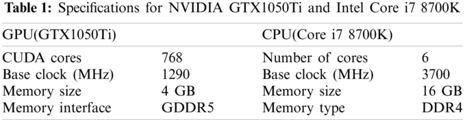
To evaluate the impact of GPUs and CPUs on the performance of our program, we run it on a PC where a NVIDIA GTX 1050Ti GPU and a Core i7 8700K CPU (Intel, Santa Clara, CA, USA) are installed. The prices of the GPU and CPU are about $130 and $430, respectively. The price of the entire PC is about $1250. The specifications for the GPU [35] and CPU [36] are shown in Tab. 1 so that the performance can be appropriately estimated. For fair evaluation, the GPU and CPU both run on the base clock. The Visual Studio 2013 (Microsoft, Redmond, WA, USA) is used to build the program. The processing times shown in Tabs. 3–5 are approximate.

A software tool Field II [37,38] is used to model a 38.4 mm linear array with 128 elements (element width = 0.28 mm, pitch = 0.3 mm, kerf = 0.02 mm, height = 5 mm) and synthesize a phantom. The elevation focus of this array is set to 30 mm. Two cycles of Hanning weighted sinusoidal pulse with 6.5 MHz center frequency are modeled as the excitation pulse. In addition, the sample frequency is set to be 120 MHz.

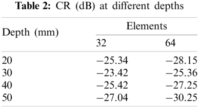
The synthesized phantom, where 200000 scatterers are randomly distributed in a 40×10×65 mm3 volume, consists of four point targets and four anechoic cysts whose radius is 3 mm. The points and cysts are located at the depth of 20, 30, 40 and 50 mm, respectively. The number of transmit elements is 32, and the transmission focal depth is 30 mm. There are 128 scan lines, and the numbers of receiving elements are 32 and 64, respectively. In the case of the mixture of the GPU and CPU, 80 lines are reconstructed on the GPU, and 48 lines are synthesized on the multi-core CPU.

The reconstructed images are shown in Fig. 6, where we can see that the Fig. 6b has high quality. The points in Fig. 6a are larger than those in Fig. 6b, which means a wider main lobe when 32 elements are used to receive signals. Compared to Fig. 6b, the cysts in Fig. 6a are also more blurred. It can be seen from Fig. 7, which shows the lateral cross sections at different depth, that the main lobe is narrower and side lobe is lower when 64 elements are used to receive signals. This is also consistent with what we observed in Fig. 6. In order to quantitatively measure the contrast, the Contrast Ratio (CR) is evaluated by [39]

where the μcyst and μbck are the mean intensities (before log-compression) of the cyst (red box in Fig. 6a) and background (white box in Fig. 6a), respectively. The corresponding CR values at different depths are shown in Tab. 2, which also indicates that adopting wider receiving aperture can get better value, but the frame rate will decrease.

Figure 6: Reconstructed simulated image using (a) 32 elements and (b) 64 elements to receive signals. All images are shown in a dynamic range of 60 dB

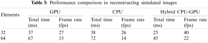
The performance comparison is shown in Tab. 3. We can observe that the GPU and the multi-core CPU have similar performance on the system. However, if the GPU and the CPU are used in mixture, the performance is significantly improved. Compared to a single GPU or CPU, the frame rate is increased by about 47%–48%.

Figure 7: Lateral cross sections at the depth of (a) 20 mm, (b) 30 mm, (c) 40 mm and (d) 50 mm

To estimate the performance of our proposed method on the experimental data, we used a medical ultrasound machine iNSIGHT 37C (Saset, Chengdu, China) to get the RF data by scanning a Multi-purpose Multi-tissue ultrasound phantom (Model 040GSE. CIRS INC., Norfolk,Virginia, 23513, USA). The center frequency and sample rate are 10 and 40 MHz, respectively. The number of scan lines in this experiment is 216, and there are 2560 points on each line. When we simultaneously run the beamformer on the GPU and CPU, 130 scan lines are reconstructed on the GPU, and 86 scan lines are synthesized on the CPU.

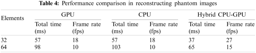
Fig. 8 displays the reconstructed phantom images. Compared to Fig. 8a, the quality of Fig. 8b is better. The CR values are calculated by using Eq. (16), and the μcyst and μbck are the mean intensities of the target (black box in Fig. 8a) and background (red box in Fig. 8a), respectively. When 64 elements are used to receive signals the CR value is 11.02 dB, and the corresponding value is 9.40 dB when 32 elements are used to receive signals. Tab. 4 illustrates the performance comparison. The frame rate of the hybrid solution is increased by about 50% in comparison with a single GPU.

Figure 8: Reconstructed phantom images using (a) 32 elements and (b) 64 elements to receive signals. All images are shown in a dynamic range of 60 dB

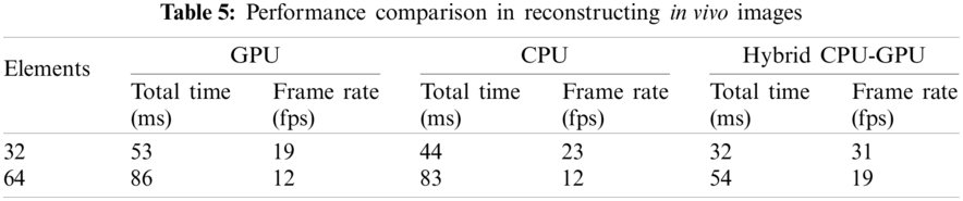
The in vivo data was acquired also by using the medical ultrasound machine iNSIGHT 37C. The number of scan lines is also 216, and there are 2048 points on each line. During the beamforming process, 130 lines are reconstructed on the GPU, and 86 lines are synthesized on the CPU. This is the same as the phantom experiment.

The reconstructed images of superficial tissue are displayed in Fig. 9. The image quality of Fig. 9b is higher than that of Fig. 9a, because more number of elements are used to receive signals. The performance comparison is illustrated in Tab. 5, where we can see that adopting the hybrid CPU-GPU gets a significant improvement in performance, and the frame rate is improved by about 58%–63% in comparison with using a GPU alone. The frame rate is about 30 fps, when 32 elements are used to receive signals. It means that this approach may be applied to ultrasound diagnosis of superficial organ.

Figure 9: Reconstructed in vivo images using (a) 32 elements and (b) 64 elements to receive signals. All images are shown in a dynamic range of 60 dB

The beamformer is one of the most critical components in an ultrasound imaging system. Among many algorithms, the DMAS excels at improving the image resolution and contrast. Thus, we tried to make this algorithm closer to practical application. We will summarize our work from two aspects.

The first purpose of this work is to lower the computational complexity of DMAS beamforming algorithm, and make it closer to practical application. The DMAS is based on the correlation operation [40], which is widely used in image processing. However, due to a group of nested loops in DMAS, the computational complexity is O(N2). Without reducing the complexity, it is hard to implement this algorithm on a real time system. Thus, we transformed the loop into some vector operations to lower the complexity. In our method, the computational complexity is O(N), because there are not any nested loops. Even without the support of parallel computation, our proposed method is also faster than the original algorithm. However, our proposed method and the other one introduced in [8] have similar performance.

The second objective is to implement the DMAS algorithm. As mentioned earlier, GPU-based beamforming technology is becoming more and more common. Therefore, our study is also based on GPUs. However, we combine a GPU with a multi-core CPU to accomplish this task rather than using a GPU alone. In this way, the computation power of multi-core CPU has also been utilized. We exploited streams to make the kernel execution overlap with the data transfer in the GPU programming. In addition, performance of page-locked memory used in the stream is also higher than the standard pageable memory [34]. Based on these two points, the time consumed by data copying can be efficiently decreased. On the other hand, as part of the computation is executed by the CPU, the work that the GPU needs to accomplish is consequently reduced. Moreover, there is an interesting thing in our tests. The multi-core CPU can get similar performance with the GPU in each comparison. However, the price of the CPU is more than 3 times that of the GPU. If a GPU of the same price is used, its computing power will be much higher than that of the CPU. In massive data processing, the GPU is the protagonist, while the CPU is the supporting role. Therefore, the performance of the GPU is considered as the benchmark. The results show that our proposed method can get significant improvement. On the test platform, the performance of the strategy of mixing a GPU and a multi-core CPU is increased by about 47%–63% compared to using a GPU alone.

In our test, we respectively used 32 elements and 64 elements to receive the signals. Because the amount of data to be processed in these two cases is not the same, the frame rate is different. The typical frame rate is about 30–40 fps in ultrasound B-mode imaging [5]. In our tests, when 32 elements are used to receive signals, the frame rate can basically meet this requirement. If the aperture is widened (which means 64 elements are used), the frame rate drops. However, the image quality will be better. Therefore, the best result is that the frame rate can be guaranteed even when the amount of data is large. This is also a problem that we need to address in our follow-up work. In addition, we will try to test its performance on other platforms without increasing the cost, and continuously optimize our program.

Acknowledgement: We thank the reviewers for their suggestions. We also thank the Saset (Chengdu) Inc., China for their support.

Funding Statement: This work was supported by the Science and Technology Research Program of Chongqing Municipal Education Commission (Grant No. KJQN201801606), the Natural Science Foundation Project of CQ CSTC (cstc2017jcyjAX0092), the Scientific Research Program of Chongqing University of Education (Grant Nos. KY201924C, 2017XJZDWT02), the Science and Technology Research Program of Chongqing Municipal Education Commission (Grant No. KJ1601410), the Project ‘Future School (Infant Education)’ of National Center For Schooling Development Programme of China (Grant No. CSDP18FC2202), the Chongqing Electronics Engineering Technology Research Center for Interactive Learning, and the Chongqing Big Data Engineering Laboratory for Children.

Conflicts of Interest: The authors declare that they have no conflicts of interest to report regarding the present study.

References

Matrone, G., Savoia, A. S., Magenes, G. C. G., & Magenes, G. (2015). The delay multiply and sum beamforming algorithm in ultrasound B-mode medical imaging. IEEE Transactions on Medical Imaging, 34(4), 940-949. [Google Scholar] [CrossRef]
Lim, H. B., Nhung, N. T., Li, E. P., & Thang, N. D. (2008). Confocal microwave imaging for breast cancer detection: Delay-multiply-and-sum image reconstruction algorithm. IEEE Transactions on Biomedical Engineering, 55(6), 1697-1704. [Google Scholar] [CrossRef]
Park, J., Jeon, S., Meng, J., Song, L., & Lee, J. S. (2016). Delay-multiply-and-sum-based synthetic aperture focusing in photoacoustic microscopy. Journal of Biomedical Optics, 21(3), 36010. [Google Scholar] [CrossRef]
Matrone, G., Ramalli, A., Savoia, A. S., Tortoli, P., & Magenes, G. (2017). High frame-rate, high resolution ultrasound imaging with multi-line transmission and filtered-delay multiply and sum beamforming. IEEE Transactions on Medical Imaging, 36(2), 478-486. [Google Scholar] [CrossRef]
Matrone, G., Savoia, A. S., Magenes, G. (2016). Filtered delay multiply and sum beamforming in plane-wave ultrasound imaging: Tests on simulated and experimental data. 2016 IEEE International Ultrasonics Symposium. Tours, France.
Kang, J., Yoon, C., Lee, J., Kye, S. B., & Lee, Y. (2016). A system-on-chip solution for point-of-care ultrasound imaging systems: Architecture and ASIC implementation. IEEE Transactions on Biomedical Circuits and Systems, 10(2), 412-423. [Google Scholar] [CrossRef]
Jensen, J. A., Holten-Lund, H., Nilsson, R. T., Hansen, M., & Larsen, U. D. (2013). SARUS: A synthetic aperture real-time ultrasound system. IEEE Transactions on Ultrasonics, Ferroelectrics, and Frequency Control, 60(9), 1838-1852. [Google Scholar] [CrossRef]
Ramalli, A., Dallai, A., Bassi, L., Scaringella, M., Boni, E. et al. (2017). High dynamic range ultrasound imaging with real-time filtered-delay multiply and sum beamforming. 2017 IEEE International Ultrasonics Symposium. Washington DC, USA.
Chen, J., Yu, A. C. H., So, H. K. H. (2012). Design considerations of real-time adaptive beamformer for medical ultrasound research using FPGA and GPU. 2012 International Conference on Field-Programmable Technology, pp. 198–205. Seoul, South Korea.
Kirk, D. B., Hwu, W. W. (2010). Programming massively parallel processors: A hands-on approach. San Francisco, USA: Morgan Kaufmann.
NVIDIA (2009). NVIDIA CUDA architecture (version 1.1). https://developer.download.nvidia.cn/compute/cuda/docs/CUDA_Architecture_Overview.pdf.
Romero, D., Martinez, O., Martin, C. J., Higuti, R. T., Octavio, A. (2009). Using GPUs for beamforming acceleration in SAFT imaging. 2009 IEEE International Ultrasonics Symposium, pp. 1334–1337. Roma, Italy.
Yiu, B. Y. S., Tsang, I. K. H., Yu, A. C. H. (2010). Real-time GPU-based software beamformer designed for advanced imaging methods research. 2010 IEEE International Ultrasonics Symposium, pp. 1920–1923. San Diego, California, USA.
Yiu, B. Y. S., Tsang, I. K. H., & Yu, A. C. H. (2011). GPU-based beamformer: Fast realization of plane wave compounding and synthetic aperture imaging. IEEE Transactions on Ultrasonics, Ferroelectrics, and Frequency Control, 58(8), 1698-1705. [Google Scholar] [CrossRef]
Hanseny, J. M., Schaa, D., Jensen, J. A. (2011). Synthetic aperture beamformation using the GPU. 2011 IEEE International Ultrasonics Symposium, pp. 373–376. Orlando, Florida, USA.
Åsen, J. P., Buskenes, J. I., Nilsen, C. I. C., Austeng, A., & Holm, S. (2014). Implementing Capon beamforming on a GPU for real-time cardiac ultrasound imaging. IEEE Transactions on Ultrasonics, Ferroelectrics, and Frequency Control, 61(1), 76-85. [Google Scholar] [CrossRef]
Yiu, B. Y. S., & Yu, A. C. H. (2015). GPU-based minimum variance beamformer for synthetic aperture imaging of the eye. Ultrasound in Medicine & Biology, 41(3), 871-883. [Google Scholar] [CrossRef]
Hyun, D., Trahey, G. E., Dahl, J. J. (2013). Vivo demonstration of a real-time simultaneous B-mode/spatial coherence GPU-based beamformer. 2013 IEEE International Ultrasonics Symposium, pp. 1280–1283. Prague, Czech Republic.
Hyun, D., Li, Y. L., Steinberg, I., Jakovljevic, M., Klap, T. et al. (2019). An open source GPU-based beamformer for real-time ultrasound imaging and applications. 2019 IEEE International Ultrasonics Symposium, pp. 20–23. Glasgow, Scotland.
Peng, B., Wang, Y., Hall, T. J., & Jiang, J. (2017). A GPU-accelerated 3-D coupled subsample estimation algorithm for volumetric breast strain elastography. IEEE Transactions on Ultrasonics, Ferroelectrics, and Frequency Control, 64(4), 694-705. [Google Scholar] [CrossRef]
Wen, T., Li, L., Zhu, Q., Qin, W., & Gu, J. (2017). GPU-accelerated kernel regression reconstruction for freehand 3D ultrasound imaging. Ultrasonic Imaging, 39(4), 208-223. [Google Scholar] [CrossRef]
Chee, A. J. Y., Yiu, B. Y. S., & Yu, A. C. H. (2017). A GPU-parallelized eigen-based clutter filter framework for ultrasound color flow imaging. IEEE Transactions on Ultrasonics, Ferroelectrics, and Frequency Control, 64(1), 150-163. [Google Scholar] [CrossRef]
Peng, B., Luo, S., Xu, Z., & Jiang, J. (2019). Accelerating 3-D GPU-based motion tracking for ultrasound strain elastography using sum-tables: Analysis and initial results. Applied Sciences, 9(10), 1991. [Google Scholar] [CrossRef]
Mohammed, M. A., Al-Khateeb, B., Rashid, A. N., Ibrahim, D. A., & Abd Ghani, M. K. (2018). Neural network and multi-fractal dimension features for breast cancer classification from ultrasound images. Computers & Electrical Engineering, 70(1), 871-882. [Google Scholar] [CrossRef]
Lu, J., Millioz, F., Garcia, D., Salles, S., & Liu, W. (2020). Reconstruction for diverging-wave imaging using deep convolutional neural networks. IEEE Transactions on Ultrasonics, Ferroelectrics, and Frequency Control, 67(12), 2481-2492. [Google Scholar] [CrossRef]
Nguyen, T. N., Podkowa, A. S., Park, T. H., Miller, R. J., & Do, M. N. (2021). Use of a convolutional neural network and quantitative ultrasound for diagnosis of fatty liver. Ultrasound in Medicine & Biology, 47(3), 556-568. [Google Scholar] [CrossRef]
Hansen, J. M., Hemmsen, M. C., Jensen, J. A. (2011). An object-oriented multi-threaded software beamformation toolbox. SPIE Medical Imaging. Lake Buena Vista (Orlando), Florida, USA.
Kjeldsen, T., Lassen, L., Hemmsen, M. C., Kjær, C., Tomov, B. G. et al. (2014). Synthetic aperture sequential beamforming implemented on multi-core platforms. 2014 IEEE International Ultrasonics Symposium, pp. 2181–2184. Chicago, Illinois, USA.
Lok, U. W., Song, P., Trzasko, J. D., Borisch, E. A., Daigle, R. et al. (2018). Parallel implementation of randomized singular value decomposition and randomized spatial downsampling for real time ultrafast microvessel imaging on a multi-core CPUs architecture. 2018 IEEE International Ultrasonics Symposium. Kobe, Japan.
Pacheco, P. (2011). An introduction to parallel programming. San Francisco, USA: Morgan Kaufmann.
OpenMP, A. R. B. (2018). Open MP application programming interface (version 5.0). https://www.openmp.org/wp-content/uploads/OpenMP-API-Specification-5.0.pdf.
So, H. K. H., Chen, J., Yiu, B. Y. S., & Yu, A. C. H. (2011). Medical ultrasound imaging: To GPU or not to GPU?. IEEE Micro, 31(5), 54-65. [Google Scholar] [CrossRef]
NVIDIA (2018). CUDA C Programming Guide (v9.2). https://docs.nvidia.com/cuda/archive/9.2/pdf/CUDA_C_Programming_Guide.pdf.
Sanders, J., Kandrot, E. (2010). CUDA by example: An introduction to general-purpose GPU programming. Boston, Massachusetts: Addison-Wesley.
NIVIDIA (2020). NVIDIA GTX 1050 specification. https://www.nvidia.com/en-us/geforce/10-series/.
Intel (2020). Intel Core i7-8700K processor specifications. https://ark.intel.com/content/www/us/en/ark/products/126684/intel-core-i7-8700k-processor-12m-cache-up-to-4-70-ghz.html.
Jensen, J. A., & Svendsen, N. B. (1992). Calculation of pressure fields from arbitrarily shaped, apodized, and excited ultrasound transducers. IEEE Transactions on Ultrasonics, Ferroelectrics, and Frequency Control, 39(2), 262-267. [Google Scholar] [CrossRef]
Jensen, J. A. (1996). Field: A program for simulating ultrasound systems. Medical & Biological Engineering & Computing, 4(Supplement 1), 351-353. [Google Scholar]
Lediju, M. A., Trahey, G. E., Byram, B. C., & Dahl, J. J. (2011). Short-lag spatial coherence of backscattered echoes: Imaging characteristics. IEEE Transactions on Ultrasonics, Ferroelectrics, and Frequency Control, 58(7), 1377-1388. [Google Scholar] [CrossRef]
Iqbal, M. S., Ahamd, I., Asif, M., Kim, S. H., & Mehmood, R. M. (2020). Drug investigation tool: Identifying the effect of drug on cell image by using improved correlation. Software: Practice and Experience, 51(2), 1-11. [Google Scholar] [CrossRef]